Simple Physical Interactions Yield Social Self-Organization in Honeybees

1 Introduction

Complex adaptive systems (CAS) are ubiquitous. They include diverse systems such as social networks, Earth’s climate, or its ecosystems [1, 2], but all CAS have specific properties and features in common: They are comprised of many independent agents whose loosely coupled and local interactions on the microscopic system level lead to emergent outcomes that are observable on the macroscopic system level. These macroscopic outcomes often happen surprisingly suddenly, e.g., phase transitions, which can profoundly alter the overall system’s properties. These system changes are not sufficiently predictable by looking only at the microscopic individual behavior [3]. Similar phenomena can be observed in eusocial insect colonies, which possess all the typical characteristics of CAS [4]. The abilities of honeybee colonies (such as the western honeybee Apis mellifera L.) allow colony adaptation on various levels by altering or modulating the interaction network that emerges between the individuals. These properties involve many nonlinear feedback loops with significant time constants (delays). These properties of system ingredients are textbook examples of prerequisites for complex behavior arising from very simple interaction patterns [5, 6]. While these functional components may easily lead to chaotic behaviors, the existence of balancing feedback loops within social insect colony systems yields homeostasis and resilience through mechanisms of social self-regulation and self-organization [7]. Ultimately, these colonies can be seen as super-organisms: as a collective, they manage to navigate the delicate balance between complexity-induced chaos and homeostatic self-regulation, a property that is seen as a characteristic of organisms and of life itself [8]. This residing on the edge between chaos and order makes social insect colonies in general, and honeybee colonies specifically, an excellent model system for complex but not chaotic CAS.

We examined the CAS of honeybees by a set of down-scaled laboratory experiments to keep the complexity of the study system within tractable bounds but still large enough to show interesting phenomena, such as collective decision-making, symmetry breaking, and biasing effects through informed leadership within the collective. We focused on how group size, environmental conditions, environmental dynamics, and local availability of information affect the individual and collective decision-making within this CAS.

Therefore, we studied groups of young honeybees, which already show complex social behaviors, e.g., in the collective thermotaxis where bees are able to collectively distinguish local from global thermal optima in complex thermal environments [9], based on simple individual processes [10]. The temperature-based self-localization behavior and the collective decision-making of young bees in complex and dynamic temperature fields of the brood nest are crucial components of the self-regulatory feedback loops of the colony. These mechanisms are governed by physical environmental stimuli that are capable of modulating the microscopic behaviors of the bees, e.g., their motion speed or their ability to preferably stay longer at places with specific environmental conditions.

Our focal research question in the presented work is as follows: Can we explain naturally observed examples of complex group-level behavior (e.g., collective thermotaxis) in complex adaptive systems (e.g., honeybees) as an emergent phenomenon arising from simple microscopic individual motion principles and simple interaction mechanisms? We here restrict ourselves to study the simplest set of mechanisms to allow us the building and parametrization of a simple but complex-enough model that is able to predict a rich set of empirical data that are collected on these CAS. This model is able to predict the emergence of collective taxis, and also the arising collective decision-making and symmetry breaking phenomena with respect to specific environmental configurations and dynamics. We further consider the social context in these processes, because it may be modulated by group members that have additional information or follow specifically different roles than our modeled agents. These predictions are made by a simple difference equation model that we develop here based on our empirical data. We used two different methods to solve the model: a mechanistic top-down approach using the forward Euler method and a bottom-up approach using an individual-based Monte Carlo simulation.

To understand the complex link between the individual microscopic behavioral repertoire of young bees and the emerging macroscopic patterns of aggregation that emerges from a collective decision-making process and the physical environment, we first conducted a set of experiments as a macroscopic evaluation of the system. We observed groups of young honey bees in static and dynamic temperature fields showing either a) one global, b) one global and one local, or c) two global optima and observed the aggregation behavior of the bees in these environments. By considering the most relevant underlying microscopic mechanisms that are the individual behaviors of young bees in such temperature fields, we ultimately developed a mathematical model that connects these two system levels. The first difference equation model is fitted to the observed empirical data collected in static temperature fields. This way the only “free parameter” our model contains, the social factor X_bee, is parametrized based on empirical data on living honeybees. Based on this parametrized difference equation model, a set of predictions is made regarding how this CAS will behave in dynamically changing environments. These predictions are then compared to empirical data for further validation of the model. Finally, we extend the model to incorporating social context and again predict the effect of biases that may arise by special actors in the collective that either pursue other goals have different limitations or possess alternative pieces of information.

2 Materials and Methods

2.1 Experiments With Honeybees

2.1.1 Animals

All experiments were conducted with young honeybees (Apis mellifera L.) aged between 1 and 30 h after hatching from their brood cells. Honeybees at this age are still ectothermic, i.e., they are not able to produce heat on their own with their wing muscles yet [11] and are therefore dependent on the appropriate thermal environment, in which they navigate actively. To collect bees with this defined age, a set of brood combs with many sealed pupae was gathered from colonies and incubated at 35°C and at a relative humidity of 60%. After hatching, the freshly emerged bees were removed from the combs and transferred to ventilated plastic containers with access to honey ad libitum to support their health and development. Each individual bee was participating only once in an experiment, and no individual with a visible handicap was used. After participating in an experiment, all bees were transferred to an identical separate container, and all bees were re-introduced into full colonies after the experiments each day.

2.1.2 Experimental Setup

Our basic experimentation setup consisted of a circular arena (with a diameter of 60 cm) that was surrounded by a plastic wall (Figure 1A). To prevent the bees from climbing the boundary, the plastic wall was coated with Teflon spray. The thermal environments were generated with either one or two ceramic heat lamps that were mounted above the arena (Figure 1B). To actively regulate the thermal environment in our setup, an array of temperature sensors was built into the acrylic glass arena floor (based on the methods described in [12]). The arena floor was covered with wax foundations that were replaced after each trial to remove any possible scent traces left behind by the bees. A standard PC controlled two digital dimmers that regulate the ceramic heat lamps by using the data from the temperature sensors. Three additional sensors were used to measure the ambient room temperature. The room temperature was kept around 29 ± 1°C by either heating with a radiator or by cooling with a portable air conditioning unit before starting each experiment. All experiments were performed under infrared light (Figure 1C), at a wavelength that is invisible for bees [13] so that we could exclude that the bees use any visual cues but were required to rely purely on their thermal sensory system and on their haptic sensory inputs when touching other bees or obstacles. Such conditions exist also in the brood area deep in the colony’s hive, where young bees usually locate themselves [14]. All experiments were recorded with an IR-sensitive camera (Figure 1D). For technical details of the individual components and the setup, see [9, 15].

FIGURE 1

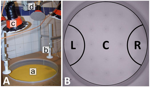
FIGURE 1. Circular temperature arena setup and evaluation zones. (A) The setup consists of a circular arena (a) with temperature sensors that are embedded in the acrylic glass floor underneath the wax foundations, surrounded by a plastic barrier. The two thermal optima are generated with ceramic heating lamps mounted above the arena (b). The setup is illuminated with lamps that are covered with filters so that only infrared light is emitted (c), and the experiments are recorded with an IR-sensitive camera (d). Furthermore, technical details can be found in Section 2.1.2 and [9]. (B) Evaluation zones: The arena was divided into three zones, with the left zone (L) and the right zone (R) representing the area under each heat lamp and the center (C) representing the area outside of these zones. For collecting the empirical data, the number of bees in each zone was determined from video recordings in either 1-minute intervals (Exp. 1–4) or at the end of each experimental run in minute 30 (Exp. 5).

2.1.3 Experiments

We carried out five different sets of experiments to gather empirical data on the honeybees’ behavioral repertoire: Three sets of experiments were conducted with groups of bees in static thermal environments to examine the influence of a static, thermally heterogeneous environment on the collective behavior. Another set of experiments was conducted with groups of bees in a dynamic environment to examine the flexibility of the collective behavior in response to sudden changes in the environmental conditions. Finally, another set of experiments was conducted with a static thermal environment and an additional social stimulus. The optimum temperature of 36°C was chosen in all experiments as it corresponds to the preferred temperature (thermal optimum) of freshly emerged, still ectothermic, honeybees [16]. To minimize the time the animals have to spend in the experimental setup, we set the runtime of experiments in stable thermal environments to 30 min to ensure enough time for the bees to explore their environment and form stable aggregations and to 105 min in dynamic thermal environments to additionally take into account the thermal inertia and the time the bees need to react to the changes in the thermal environment.

Static Thermal Environments—Experiments 1, 2, and 3

We conducted three different sets of experiments with this setting, each one with groups of 64 bees, in different configurations of static thermal environments. The bees were introduced (released from their cup) in the center of the arena, and each experimental run lasted for 30 min. In Experiment 1, we generated a thermal environment with one global optimum at 36 ± 1°C on one arena side and with a pessimum of 30 ± 1°C on the other arena side, as depicted in Figure 2A (n = 9 repetitions). In Experiment 2, we generated a more complex environment with, again, a global optimum at 36 ± 1°C on one arena side, but this time also with a local optimum at 32 ± 1°C on the opposite side of the arena as depicted in Figure 2B (n = 8 repetitions). In Experiment 3, we generated a thermal environment with two equally optimal spots at 36 ± 1°C on two opposite sides of the arena as depicted in Figure 2C (n = 6 repetitions).

FIGURE 2

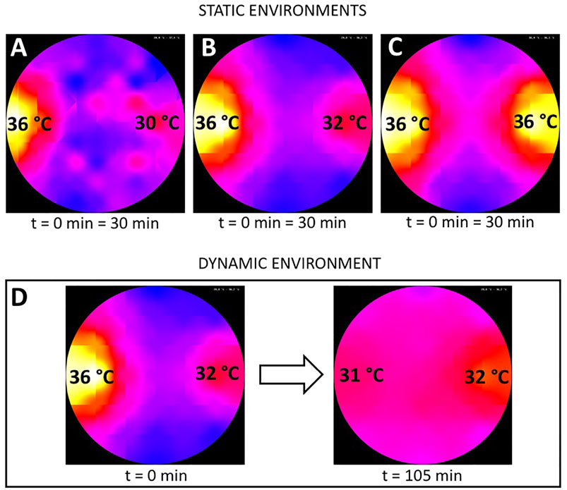
FIGURE 2. Graphical representation of the used static and dynamic thermal environments in the different experiments. (A) static environment with one global optimum of 36±1°C on the left side (used in Experiment 1), (B) static thermal environment with a global (36±1°C) optimum on the left and a local optimum (32±1°C) on the right side (used in Experiments 2 and 5), (C) static environment with two global 36±1°C optima on opposing sides of the arena (used in experiment 3) and (D) dynamic environment used in Experiment 4 with an initial configuration equal to (B) and the resulting thermal environment at the end of the experiment after switching off the heat lamp on the left side at minute 30 with the new global optimum of 32±1°C on the right side. The run-time of the experiments with static environments was 30 minutes and 105 minutes in the experiments with the dynamic environment.

FIGURE 3

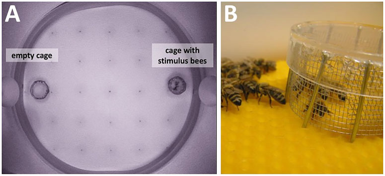
FIGURE 3. Setup for experiment 5. (A) A wire cage with a transparent top was placed under each heat lamp. The cage placed under the right heat lamp that produced the local optimum contained 5 stimulus bees while the cage on the left in the global optimum remained empty and acted as a control. (B) Close-up of the caged bees with aggregated bees around.

Dynamic Thermal Environment—Experiment 4

The experimental runs with a dynamic thermal environment were also performed with groups of 64 bees. The bees were introduced in the center of the arena, and each experimental run lasted for 105 min (n = 17 repetitions). For this experimental setup, we generated an initial environment with a global optimum at 36 ± 1°C and a local optimum at 32 ± 1°C on the opposite side of the arena, equal to the second set of experiments with a static thermal environment. Thirty minutes after introducing the bees, the heat lamp providing the 36 ± 1°C optimum was shut off while the heat lamp generating the 32 ± 1°C optimum remained at the initial setting, leading to a change in the thermal environment as depicted in Figure 2D.

Static Thermal Environment With Social Stimulus—Experiment 5

In the experimental runs with a social stimulus, we used groups of 24–25 bees that could run freely in the arena. The thermal environment was equivalent to the one used in experiment 2 with one global optimum at 36 ± 1°C and a local optimum at 32 ± 1°C on the opposite side of the arena (as depicted in Figure 2B). To provide a local social stimulus, we introduced additional bees as a local “social stimulus” that was confined to a specific location. To confine these “social stimulus” bees, we used circular cages that were built from wire mesh and covered with an acrylic glass Petri dish (3B). We put two cages in the arena, one under each heat lamp (3A), whereby the cage in the local optimum contained the five stimulus bees. The cage in the global optimum remained empty and acted as a control against effects such as the wire cage itself hypothetically acting as an attractant for the bees. The test bees were introduced in the center of the arena and could run freely in the arena, except for the space covered by the cages. Each experimental run lasted for 30 min (n = 10 repetitions).

2.1.4 Data Collection and Evaluation

The experiments were evaluated by assessing the location of the bees in specific time intervals throughout the experimental runtime. To collect the data, the area of the circular arena was subdivided into three zones: L (zone under left heat lamp), R (zone under right heat lamp), and C (remaining area; center) as depicted in Figure 1B. The left and right zones cover 11.2% of the total arena size each, corresponding to the area heated by the heat lamps. We manually counted the bees in each evaluation zone in 1-min intervals on still images from the recordings for experiments 1–4 to acquire a sufficient amount of data points for the model fitting (experiments 1–3) and to capture the dynamics in experiment 4. For experiment 5, we evaluated the number of bees in the respective zones at the end of the experimental runs (after 30 min). Each bee was attributed to the zone where most of its body was located. If a bee happened to be exactly on the evaluation line between two zones, it was attributed to the zone its thorax was located in. If a bee’s thorax was directly on the line, it was attributed to the zone it was headed to. We evaluated a total of 50 runs with this method.

To visually depict the influence of the physical stimulus (temperature) on the macroscopic distribution pattern of the bees, we indicate the expected occupancy of the different zones, assuming that the bees ignore other bees and the local temperature (uniform distribution as a null model, see also [9]), in the result graphs for the empirical data. The expected occupancy is indicated as a dotted horizontal line for the respective evaluation zone, with an expected fraction of bees of 0.112 for the right and the left zones, respectively, and 0.776 for the center, corresponding to the size ratios of the evaluation zones.

All statistical comparisons were performed using the MannWhitney U test with a significance level of 0.05, and the p values are given in parentheses where results are reported.

2.2 Method of Parameterization and Fitting of the Developed Difference Equation Model

2.2.1 Implementation of the Temperature-Dependent Waiting Time

Bees are known to often rest (wait) for some time after a bee-to-bee contact, and it is known that this behavior is affected by the local temperature [9, 17]. To represent this important mechanism in the difference equation model, we generated a waiting-time function that maps a given time-dependent temperature T(t) to a predicted waiting period duration.

This waiting time of a bee W (T(t)) is derived from empirical data collected in observations of young honeybees [18] and is described through the sigmoidal function

$W(T(t))=a\cdot tanh\left(\frac{T(t)}{b}-d\right)+e(1)$

with the parameters a = 12, b = 1.2, d = 27, and e = 13. This yields a curve that returns 1 s at 28°C and 25 s at 36°C as depicted in Figure 4A. Restricted through the lower boundary of the waiting time, we chose a time step of Δt = 1 s for our model.

FIGURE 4

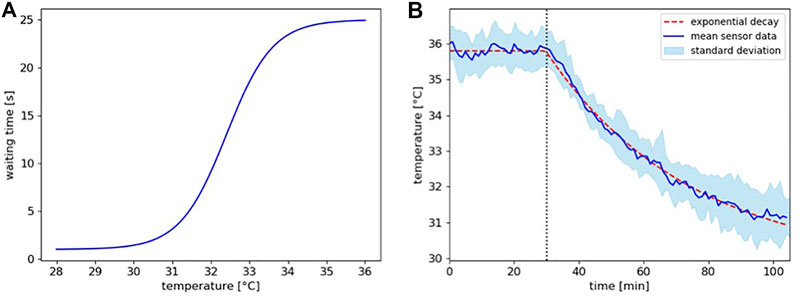
FIGURE 4. (A) Function of the implemented waiting time in dependence of the locally experienced temperature according to equation 1. (B) Temperature decay model. Shown are the mean temperature sensor data with standard deviation from the left zone overtime for the runs of experiment 4 (blue line and band) and the implemented temperature profile for the model (dashed red line). The decrease in temperature after the lamp was switched off at minute 30 (dotted vertical line) follows the characteristics of an exponential decay.

Our model needs also to be able to depict a dynamic thermal environment, i.e., the temperature decay over time that is a significant aspect in experiment 4 after the heating lamp is turned off. Thus, we used the mean temperature sensor data for the left temperature field zone from the runs of experiment 4 and fitted a temperature decay curve to the values that lie on the mean of the deviation (see Figure 4B).

2.2.2 Model Fitting

To fit our model’s difference equations, we used the proven method of least squared residuals. Here, we looked at the difference between the model’s prediction and the empirically observed mean value at equally spaced given points in time and minimized the sum of all squared residuals by numerically solving the equations while adjusting our social parameter X_bee. To find the one parameter value that suits all the conducted experiments 1, 2, and 3, we fitted the equations to the mean empirical data of all zones and experiments at once.

2.2.3 Noise Implementation

The basic behavior exhibited by most bees in a thermal field is forms of correlated random walks [10, 17, 19, 20]. To reflect this randomness in the underlying microscopic behaviors, we implemented a noise-affected term in our model. This noise is introduced to the system by multiplicative application of a time-discrete, uncorrelated, and Gaussian distributed random value (see Eq. 2) on the free parameter, the social factor X_bee, with the mean μ = 1 and a standard deviation σ = 0.25 restricting the possible values to the interval [0; 2], which is necessary to guarantee non-negativity and symmetry around the mean.

$ϵ(t)=\frac{1}{\sigma \sqrt{2\pi }}{e}^{-\frac{1}{2}{\left(\frac{t-\mu }{\sigma }\right)}^2}(2)$

3 Results

3.1 Groups of Bees in Static Thermal Environments

To examine the macroscopically observable patterns of aggregation, we conducted experiments with different static thermal environments. In experiment 1, with only one global optimum at 36°C, the majority of bees are found in the left evaluation zone at the end of the experimental runs. This zone corresponds to the global thermal optimum, and most bees are located there within 15 min. The median fraction of bees in the left zone is significantly higher than in the center zone and the right zone after 15 and after 30 min (p < 0.001, compare Figure 5A left, center, and right). Similarly, in experiment 2, with a global optimum on the left and a local optimum on the right side of the arena, the median fraction of bees at the global optimum on the left was significantly higher than the median fraction of bees in the center (p = 0.003) and at the local optimum on the right (p = 0.012) (Figure 5B left, center, and right) after 30 min. In experiment 3, with a thermal environment containing two equally warm global optima, the results in Figure 5C show no statistical difference in the median fraction of bees between the right and the left zones (p = 0.261). For this experiment, we also looked at the individual trials that show that while the groups split up approx. 50:50 in most of the trials, in 20% of the trials a strong symmetry breaking occurred, i.e. the majority of the bees aggregated on one side of the arena (see Figure 6).

FIGURE 5

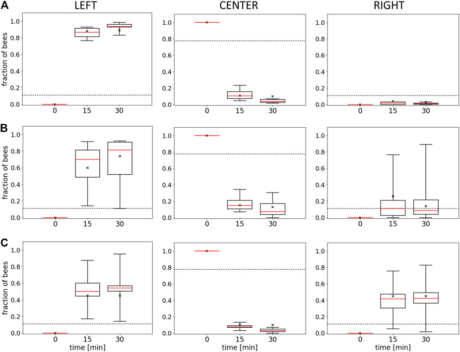
FIGURE 5. Results of Experiments 1, 2, and 3. Shown is the median fraction of bees (with Q1, Q3, minimum, and maximum) at minutes 0, 15, and 30 in the left evaluation zone (L), the center (C), and the right evaluation zone (R) for (A) Experiment 1 (L: 36±1°C, R: 30±1°C), n=9 repetitions, (B) Experiment 2 (L: 36±1°C, R: 32±1°C), n=8 repetitions, and (C) Experiment 3 (L: 36±1°C, R: 36±1°C), n=6 repetitions. The crosses indicate the model fits for each data series for the model described in the discussion section. Dotted horizontal lines indicate the expected occupancy if the bees ignored other bees and the local temperature (uniform distribution model).

FIGURE 6

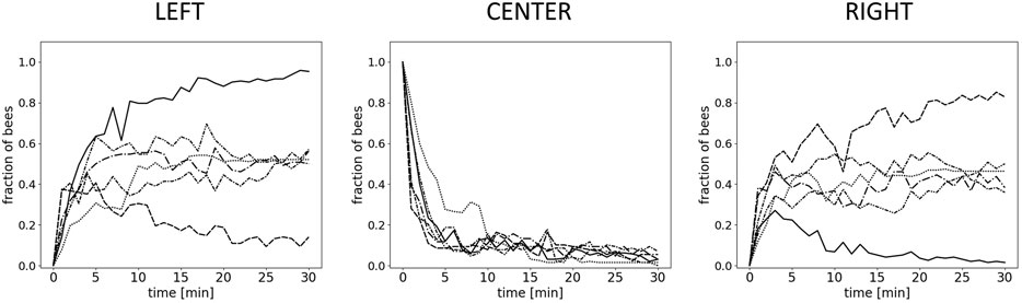
FIGURE 6. Results for Experiment 3–individual runs. Shown is the fraction of bees in 1-minute wide intervals over the whole experimental run-time (30 minutes) for each individual run (n=6 repetitions) in the left zone (36±1°C), the center, and the right zone (36±1°C).

3.2 Building a Difference Equation Model of the Observed System

Based on the empirical results we described in the previous section, we here develop a simple difference equation model in which we break down the social stimulus-based self-localization behavior into basic principles. We aim at constructing a parsimonious model with a limited set of parameters that describe the observed complex behaviors in a simple way. An overview of all model variables and parameters is given in Table 1. The model tracks the bees with conservation of mass and describes their rates of change between the three compartments that were used and are thus suggested by the empirical experiments’ analysis method: The state variable L(t) models all bees located in the left zone, the state variable R(t) models all bees located in the right zone, and the state variable C(t) models all other bees. The total number of bees is N = L(t) + C(t) + R(t), guaranteeing respect for mass conservation in the model. For the sake of simplicity, we do not explicitly model the area of the zones (and, respectively, the proportions of its boundaries) or the area a bee or a group of bees would occupy.

TABLE 1

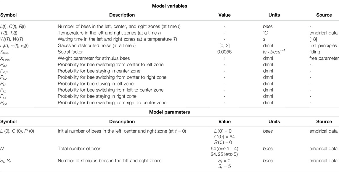
TABLE 1. Model variables and parameters.

The changes of the three state variables are then described as a system of coupled ordinary difference equations, whereby

$\frac{\mathrm{\Delta }L}{\mathrm{\Delta }t}=mee{t}_l(t)+joi{n}_l(t)-leav{e}_l(t)(3)$

models the change in the number of bees in the left zone,

$\frac{\mathrm{\Delta }R}{\mathrm{\Delta }t}=mee{t}_r(t)+joi{n}_r(t)-leav{e}_r(t)(4)$

models the change in the number of bees in the right zone, and

$C(t)=N-L(t)-R(t)(5)$

models the number of bees in the center simply by subtracting the number of bees that are in the left and right zones from the total number of bees.

These three equations are modeled following the standard mass action law, as it expresses the expected interactions of entities based on their mean densities, as it is also used in the mathematical modeling of predator-prey and host-parasite systems [21, 22], intraspecific competition [23], interspecific competition [24], the spreading of infectious diseases [25], or chemical, e.g., enzyme-substrate interactions [26].

As we aim for the simplest version of this model, we combined all individual microscopic parameters—motion behavior, sensory range, contact detection—into one single parameter that we named “social factor” X_bee. Another microscopic system-level aspect that needs to be modeled is the individual behavioral response to the locally perceived temperature and how this affects the social interaction. Young honeybees tend to stop after encountering another bee and rest for some time after such collisions, whereby the resting time is positively correlated with the local temperature [9, 17]. This temperature-dependent waiting time is represented by W(T). For the model, we assume that the bees move randomly and stop when encountering another bee with a probability determined by X_bee and that the waiting time of those individuals depends on the locally prevalent temperature [9]. The implemented waiting-time function is depicted in Figure 4A. The terms on the RHS of our equations are functions of time in our model. They express specific processes that affect the rate of change of the specific system variable on the LHS of the equation.

The functions meet_l(t) and meet_r(t) represent half of the initial center zone bees that, after interacting with each other in dependence of our social factor X_bee, form a cluster in the left and right zones equally likely and are described as

$mee{t}_l(t)=mee{t}_r(t)=\frac{1}{2}\cdot X_{bee}\cdot C{(t)}^2(6)$

The functions join_l(t) and join_r(t) represent initial center zone bees that join already present bees in the left and right zones and are described as

$joi{n}_l(t)=X_{bee}\cdot L(t)\cdot C(t)(7)$

for the left zone and

$joi{n}_r(t)=X_{bee}\cdot R(t)\cdot C(t)(8)$

for the right zone.

Finally, the functions leave_l(t) and leave_r(t) represent the bees in either zone that transition back to the center zone after their temperature-dependent waiting time has expired and are described as

$leav{e}_l(t)=\frac{L(t)}{W_l(T_l(t))}(9)$

for the left zone and

$leav{e}_r(t)=\frac{R(t)}{W_r(T_r(t))}(10)$

for the right zone.

In our empirical experiments with bees, the number of bees was kept constant in experiments 1 to 3. For the simulation runs of our model, we thus set N to a value of 64, and equivalent to the experiments, all bees were starting in the center region, therefore C (0) = N bees and L (0) = R (0) = 0 bees. The variables that represent the mean temperatures within the left and right area are set T_l(t) = 36°C and T_r(t) = 30°C, respectively, for comparison with experiment 1, to T_l(t) = 36°C on the right and T_r(t) = 32°C on the left for comparison with experiment 2 and to T_l(t) = T_r(t) = 36°C on both sides for comparison with experiment 3.

The functions that involve the waiting times W_l (T(t)) and W_r (T(t)) in the modeling of specific rates of change represent the number of bees that leave their zone of resting (Eq.(3) and (4) and transition back into the center zone (Eq.5), which can be assumed to be equal to the mean time a bee spends in this zone. This waiting duration is not directly a function of time, but a function of the local temperature, as was expressed by W (T(t)) in Eq. 1. However, the mean temperatures and thus the waiting times within the two zones are able to change in time in our experiments.

Finally, our system of coupled difference equations is numerically solved through the forward Euler method with a step size of Δt = 1.

In our model building approach, we aim at a “one fits all” model; thus, we fitted our free parameter X_bee to the empirical data set from all our experiments in static environments (experiments 1–3), aiming for a value with which the model can qualitatively (and partially even quantitatively) represent the results from all three experiments sufficiently.

Using the method described in subsection 2.2.2, we found the best fit for our free parameter with a value of $X_{bee}=0.0056\frac{1}{s\cdot bee}$. The results of this fitting are shown in Figure 7, where the empirical data (median fraction of bees, IQR, minimum, and maximum) that were used for fitting are plotted over time for experiments 1 (Figure 7A), 2 (Figure 7B), and 3 (Figure 7C) with the respective fitted model results (dashed lines).

FIGURE 7

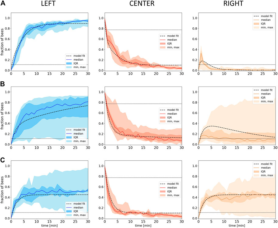
FIGURE 7. Model fitting. Shown is the fraction of bees in the different evaluation zones (Left, Center, Right) from empirical data (median with IQR, minimum and maximum) over time with the respective fitted model data (dashed lines) with the social factor X_bee of $0.0056\frac{1}{s\cdot bee}$ for (A) experiment 1 (L: 36±1°C, R: 30±1°C), n=9 repetitions (B) experiment 2 (L: 36±1°C, R: 32±1°C), n=8 repetitions and (C) experiment 3 (L: 36±1°C, R: 36±1°C), n=6 repetitions. Dotted horizontal lines indicate the expected occupancy if the bees ignored other bees and the local temperature (uniform distribution model).

3.3 Predicting Macroscopic Aggregation Patterns in Complex Environments

To test the predictive ability of the model when applied to new data, we simulated our model in resembling to the two experimental settings that were not previously used to fit the model’s parameters: experiment 4 with a dynamic thermal environment and experiment 5 with an additional social stimulus. The model predictions of these experiments can then be compared to the empirical observations for validation purposes.

3.3.1 Aggregation Patterns in a Dynamic Thermal Environment (Model Solved With the Forward Euler Method)

The empiric results from experiment 4 show that the median fraction of bees in the left zone at the optimal temperature rises in the initial phase, when this side holds a global optimum of 36°C. As soon as the heat lamp on the left is switched off in minute 30, the median fraction of bees in the left zone starts to decrease. In parallel, we find an increase in the right zone (32°C) while the median fraction of bees in the center rises only slightly (8A). As soon as the left zone starts to cool down, the unchanged right zone becomes the global optimum in the system, and the bees collectively start to aggregate in this zone. Statistical analysis of our data indicates a median fraction of bees in the left zone that is significantly higher than in the right zone at minute 30 (p < 0.001). When comparing the median fraction of bees in the left zone at minute 30 with the median fraction of bees in the right zone at the end of the experiment (minute 105), no statistical difference was found (p = 0.97). The same was found when comparing the median fraction of bees in the left zone at minute 105 and the right zone at minute 30 (p = 0.63).

To model the dynamic thermal environment from experiment 4, we implemented the time dependency via the temporal progression of the temperature T = T(t), as detailed in Section 2.2.1. Besides adding the required exponential decay of temperature in the left zone and applying noise to the system’s free parameter (see Section 2.2.3), no changes were made to the model for simulating experiment 4. As the system has three distinct possibilities for the interaction of bees (C², C ⋅ L, and C ⋅ R), we implemented three uncorrelated noise factors ϵ₁(t), ϵ₂(t), and ϵ₃(t), corresponding to Eq. 2, and with one factor for each of the three possibilities. As the bees that leave the center split up 50:50 (Eq. 6), the noise that is applied to one side needs to be reflected in the other by subtracting it from the maximum possible value that the noise can deliver, forming the term (2 − ϵ₁(t)).

After introducing the noise, the resulting cluster functions (Eqs. 6–8) are being restated as following:

$mee{t}_l(t)={ϵ}_1(t)\cdot \frac{1}{2}\cdot X_{bee}\cdot C{(t)}^2(11)$

$mee{t}_r(t)=(2-{ϵ}_1(t))\cdot \frac{1}{2}\cdot X_{bee}\cdot C{(t)}^2(12)$

$joi{n}_l(t)={ϵ}_2(t)\cdot X_{bee}\cdot L(t)\cdot C(t)(13)$

$joi{n}_r(t)={ϵ}_3(t)\cdot X_{bee}\cdot R(t)\cdot C(t)(14)$

For the prediction of the empirical data, we performed 20 individual runs with the model, with settings that match the experimental conditions: An initial static thermal environment with 36°C on the left side and 32°C on the right side, with the temperature on the left side decreasing according to the exponential decay and groups of 64 bees. For X_bee, we used the value $0.0056\frac{1}{s\cdot bee}$ as it was determined by the initial fit to data from static thermal environments.

The resulting simulation data are shown in Figure 8B: Our model generates a lower variance but predicts the dynamics in all zones quantitatively well when compared to the empirical data. The model also qualitatively captures the delay between the switching off of the heat lamp in the left zone and the decrease in the median fraction of bees, but compared to the empirical data, the delay is longer and even shows an initial increase (compare Figure 8A left and B left). Similarly to the empirical data, also in the model, the median fraction of bees is comparably low and increases slightly in the later half of the experimental runtime during the transition of bees from the left to the right side (Figure 8B). The model also qualitatively captures the increase in the number of bees in the right zone at about the point in time when the median fraction of bees on the other side starts to decrease, what also fits qualitatively well to the empirical data (Figure 8B). The median fraction of bees in the right zone after the transition at minute 105 does not significantly differ from the median fraction of bees in the left zone at minute 30 before the transition in the model data (p = 0.253). While the empirical data show no statistical significant differences when comparing the median fraction of bees in the left zone at minute 105 and in the right zone at minute 30, the model results show a significant difference for the same comparison (p < 0.001).

FIGURE 8

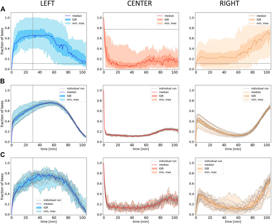
FIGURE 8. Empirical and model results from experiment 4. (A) Empirical data: Shown is the median fraction of bees (with IQR, minimum and maximum) in the different evaluation zones (Left, Center, Right) over 105 minutes experimental runtime (data collected in 1-minute intervals), n=17 repetitions. Dotted horizontal lines indicate the expected occupancy if the bees ignored other bees and the local temperature (uniform distribution). (B) Predictions of the model solved with the forward Euler method: Shown is the median fraction of bees (with IQR, minimum and maximum) in the different evaluation zones (Left, Center, Right) over an equivalent of 105 minutes experimental runtime, grey lines represent the individual model runs, n=20 repetitions. (C) Individual-based Monte Carlo simulation predictions: Shown is the median fraction of bees (with IQR, minimum and maximum) in the different evaluation zones over the experimental runtime, grey lines represent the individual model runs, n=20 repetitions. The solid vertical lines in the graphs for the left zone in (A), (B) and (C) indicate the point in time where the lamp in this zone was switched off at minute 30.

The quantitative comparison between the empirical data and the model data shows that there is no significant difference between the median fraction of bees in the experimental left zone and in the simulated left zone (p = 0.843) and also no significant difference when comparing the median fraction of bees in the experimental and in the simulated right zone (p = 0.96) at minute 30. The same was found when comparing the median fraction of bees of the experimental and of the model data in the left zone (p = 0.165) and in the right zone (p = 0.353) at minute 105.

The noise in the model that is solved with the forward Euler method produces a lower variance compared to the empirical data. We therefore simulated the same experiment with an individual-based sequential Monte Carlo method as described in the next section.

3.3.2 Aggregation Patterns in a Dynamic Thermal Environment (Individual-Based Monte Carlo Simulation)

To represent the higher variance that is shown in the experimental data, we introduce a sequential and individual-based Monte Carlo simulation, in which the difference equations are described by the probabilities for each bee to transition into a neighboring zone (see Figure 9).

FIGURE 9

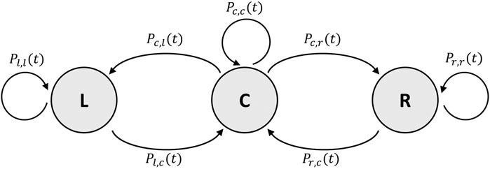
FIGURE 9. Finite state machine of the individual-based Monte Carlo simulation. States and transitions as described in Section 3.3.2.

The probability P for a bee to transition from the center C to the left zone L is defined as P_c,l(t) = X_bee ⋅ (L(t) + 0.5 ⋅ C(t)) and, respectively, to the right zone R as P_c,r(t) = X_bee ⋅ (R(t) + 0.5 ⋅ C(t)). The probability for a bee to leave the left zone is defined as P_l,c(t) = 1/W_l(t) and as P_r,c(t) = 1/W_r(t) to leave the right zone. The probabilities P_l,l(t), P_r,r(t), and P_c,c(t) are the counter-probabilities and are defined as P_l,l(t) = 1 − P_l,c(t) for the left zone, P_r,r(t) = 1 − P_r,c(t) for the right zone, and P_c,c(t) = 1 − P_c,l(t) − P_c,r(t) for the center zone.

The results are depicted in Figure 8C and show that the variance produced by the individual-based Monte Carlo simulation is greater than the variance produced by the model solved with the forward Euler method (Figure 8B) and more similar to the empirical data shown inFigure 8A.

Similarly to the predictions made by the model solved with the forward Euler method, the median fraction of simulated bees in the right zone after the transition at minute 105 does not significantly differ from the median fraction of bees in the left zone at minute 30 before the transition (p = 0.291). As it is the case for the results of the model solved with the forward Euler method, and in contrast to the empirical results, the results from the individual-based Monte Carlo simulation also show a significant difference when comparing the median fraction of bees in the left zone at minute 105 and in the right zone at minute 30 (p < 0.001).

The quantitative comparison between the empirical data and the model data shows that there is no significant difference between the median fraction of bees in the experimental left zone and in the simulated left zone (p = 0.772) and also no significant difference when comparing the median fraction of bees in the experimental and in the simulated right zone (p = 0.437) at minute 30. The same was found when comparing the median fraction of bees of the experimental and of the model data in the right zone at minute 105 (p = 0.279), while there is a significant difference between the median fraction of bees of the experimental data and the model data in the left zone at minute 105 (p = 0.002).

3.3.3 Aggregation Patterns in a Static Environment With an Added Social Stimulus

The results from experiment 2 reported in Section 3.1 show that the bees are collectively able to distinguish the global from the local optimum with the majority of the bees found in the right zone at 36°C after 30 min (Figure 5B). Based on these findings, we studied whether or not this collective decision-making process can be biased by a social stimulus in the local optimum in the same thermal environment used for experiment 2. Therefore, we tested groups of 24–25 bees and additionally introduced five bees that were confined in the local optimum. The empirical results for this experiment are shown in Figure 10A (blue data set). To show the effect of the social stimulus on the macroscopic behavior, we compare it with data from comparable experiments without a social stimulus, redrawn from [9] (red data set), where experiments with groups of 24 bees in the same static thermal environment were reported.

FIGURE 10

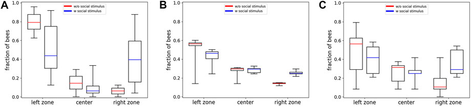
FIGURE 10. Empirical and model results from experiment 5. (A) Empirical data: Shown is the comparison of the median fraction of bees (with Q1, Q3, minimum and maximum) in the different evaluation zones (Left, Center, Right) at minute 30 between experiments with an added social stimulus in the local optimum (blue, n=10 repetitions) and experiments without this social stimulus (red, data redrawn from [9], n=8 repetitions). (B) Predictions of the model solved with the forward Euler method: Comparison of the median fraction of bees (with Q1, Q3, minimum, and maximum) in the different zones (Left, Center, Right) at minute 30 between runs with an added social stimulus in the local optimum (blue, n=10 repetitions) and experiments without this social stimulus (red, n=10 repetitions). (C) Predictions of the individual-based Monte Carlo simulation: Comparison of the median fraction of bees (with Q1, Q3, minimum, and maximum) in the different zones (Left, Center, Right) at minute 30 between runs with an added social stimulus in the local optimum (blue, n=10 repetitions) and experiments without this social stimulus (red, n=10 repetitions).

These results show that the median fraction of bees in the global optimum is significantly lower in experiments with a social stimulus compared to experiments without a social stimulus (p = 0.036, compare boxplots in Figure 10A left zone), while the median fraction of bees is significantly higher in the local optimum in experiments with a social stimulus (caged bees) compared to the experiments without caged bees (p = 0.009, compare boxplots in Figure 10A right zone); thus, the data show that a social stimulus has an influence on the overall macroscopic aggregation pattern of the bees.

To be able to predict the results of the empirical experiment with a social stimulus with our model, we had to implement an equivalent for these “caged bees.” We did this by modifying our difference equation system and included an additional term that takes into account the number of stimulus bees S_l and S_r and another parameter different from X_bee, the “social seed” parameter X_seed, that acts as a weighting value for S_l and S_r. We can see these bees as being “informed agents” or acting as social “influencers” in the collective decision-making process. We assume that a stimulus bee weighs as much as a free bee in the calculations, thus X_seed = 1.0. The three difference equations for the three zones are being extended by introducing the following functions to the left and right zones, respectively:

$socia{l}_l(t)={ϵ}_2(t)\cdot X_{bee}\cdot C(t)\cdot X_{seed}\cdot S_l(15)$

$socia{l}_r(t)={ϵ}_3(t)\cdot X_{bee}\cdot C(t)\cdot X_{seed}\cdot S_r(16)$

Furthermore, while all other empirical data are based on experiments with groups of 64 bees, the experiments with caged bees were performed with groups of 24–25 bees plus five bees in the cage at the local optimum. The model was previously fitted to a group size of 64 bees and was not refitted to adapt for the smaller group size, and thus the lower population density, in the same setup.

The simulation results with the extended model solved with the forward Euler method are depicted in Figure 10B. To show the effect of the implemented social stimulus, we compare the results with simulations using groups of 24 bees without the social stimulus term. The median fraction of bees in the global optimum is predicted to be significantly lower in runs with a social stimulus acting at the zone with the local optimum on the opposite arena side, compared to runs without a social stimulus acting on the other side (p < 0.001, compare boxplots in Figure 10B left zone). The median fraction of bees is predicted to be significantly higher in the local optimum zone in runs with the social stimulus presents compared to the runs without the social stimulus (p < 0.001, compare boxplots in Figure 10B right zone).

The statistical analysis shows that there is no significant difference between the empirical and the model data with social stimulus in the median fraction of bees in the left zone (p = 0.734) as well as in the right zone (p = 0.273, compare Figures 10A,B blue data series in left zone and A and B blue data series in right zone). The prediction of the model solved with the forward Euler method is therefore quantitatively comparable to the empirical data.

The resulting distributions of 10 exemplary runs of the individual-based Monte Carlo simulation are shown in Figure 10C. The comparison between the results from the model solved with the forward Euler method and the individual-based Monte Carlo simulation shows that there is no significant difference between the median fraction of bees in the left zones (p = 0.623, compare boxplots of left zone in Figures 10B,C) or the right zones (p = 0.053, compare boxplots of right zones in Figures 10B,C).

4 Discussion and Conclusions

This study shows that groups of young bees, in contrast to the highly variable individual thermotactic behavior of young bees [10], reliably manage to aggregate at a global thermal optimum amongst the accessible set of options. It provides novel empirical findings about symmetry-breaking events and shows the flexibility and dynamics of the bees’ collective thermotactic behavior in dynamic environments and the influence of social cues on the collective decision-making. The simple model of this collective thermotactic behavior, which was step-wise developed here (Figure 11), uses only one free parameter that combines all microscopic individual parameters. Despite its simplicity, the model is able to capture the bees’ aggregation patterns of all tested scenarios. The model shows that the prerequisites for explaining the abilities of the bee collective by means of social interactions are much smaller than an equally well-performing individual problem-solving would require. Thus, the observed behavior is a clear candidate for a phenomenon known as “swarm intelligence” [5, 27–29]. This phenomenon has aspects of emergence and exhibits interesting micromacro bridging at its core, a simple model to describe such systems is therefore of great value.

FIGURE 11

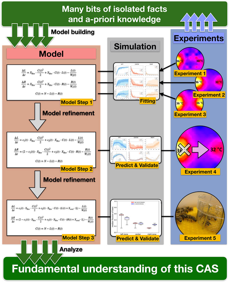
FIGURE 11. Graphic representation of our scientific workflow and concept. Based on empiric results from laboratory experiments and a-priory knowledge (e.g., temperature-dependent waiting time), we built a simple model of the collective thermotaxis in honeybees that describe the change of the number of bees in the three zones with three coupled difference equations and combined all individual microscopic parameters into the free parameter X_bee in Model Step 1. We then fitted the model to data from 3 different laboratory experiments to determine a single value for the free parameter X_bee. After this fitting, the model was further refined by adding noise to the free parameter X_bee (Model Step 2). To test the predictive ability and validate the model, we compared the simulation results to a laboratory experiment with a dynamic gradient (Experiment 4) using the previously fitted value for X_bee. In Model Step 3, we introduced the “social seed” parameter X_bee to simulate caged bees equivalent to Experiment 5. Starting with single empirical facts, we gained a fundamental understanding of the CAS by gradually developing our model and using subsequent empirical experiments to validate previous model building steps.

The empirical data show that local optima do not trap a significant amount of bees; thus, we can reject that the bees simply perform an individual uphill walk in the temperature gradient. In addition, we deduce from our experiments with two equal optima in the environment an informative result: The analysis of the individual runs shows that the bees sometimes exhibit strong symmetry breaking and collectively choose one of the two equally favorable options. Such symmetry breaking is, for example, known to happen in choice experiments with ants, where small random variations in trail laying are amplified and lead to a collective choice for one of two identical shelter options [6]. We assume a similar effect in our focal honeybee system: Whenever more bees randomly move to one side of the arena, more small initial aggregations may emerge faster on this side than on the other and increase the probability of additional bees joining there. Furthermore, empirical research on the individual motion behavior in this experimental setting (e.g., tracking individual trajectories) will be necessary to learn more about the prerequisites for symmetry breaking in this system.

We further showed the adaptability of the collective thermotaxis in honeybees in dynamic environments as the bees were capable of selecting a previously neglected less warm place when the environment changed. This shows that bees are not exclusively searching for their thermal optimum of 36°C, but instead dynamically and adaptively choose the best available option in their environment at a given time collectively, while they simultaneously try to stay together as a group. This is demonstrated by introducing a “social seed” to bias the group decision: Although the bees usually would choose the warmest area in the environment, an additional social stimulus unfolds a significant influence onto the overall collective behavior and ultimately has a tendency of drawing the bees to a comparably suboptimal temperature zone. The caged bees can exert some sort of direct physical influence, e.g., via olfactory or ground-vibrational cues. Additionally, they also exert some indirect influence via the system’s behavioral feedback loops, e.g., by increasing the stopping probability. Such effects have also been observed in swarms of robots that perform similar behavioral programs [19]. Analogous to our experiments, some immobile robots are placed at a local optimum. These immobile robots simply increase the stopping probability there, what induces a similar change in the macroscopic swarm behavior without the need of emitting any additional cues. This indicates that no direct influence from the caged bees is necessary, just their plain local presence was sufficient to emphasize local behavioral feedback loops to draw the group to the local temperature optimum. Although the robot swarm example shows that communication via direct signal exchange is not necessary to achieve such effects, the bees could still exchange signals, e.g., to achieve a faster or more stable effect. Also, more indirect density-dependent amplifiers are possible. The temperature-dependent waiting time could be additionally modulated by cluster size, as it was shown for the aggregation behavior of cockroaches [30]. A bee could wait increasingly longer the more bees it is surrounded by, what would further stabilize aggregations as soon as a certain number of bees are aggregated.

The results of our experiments suggest that the ability to solve the given sets of problems cannot be explained by simple individual behavioral programs such as a simple gradient ascent, probabilistic choosing, or a specific temperature threshold. Thus, solving the problem on an individual level would require a sophisticated behavior, assuming several sophisticated (cognitive) abilities: good sensor discrimination, memory, self-localization in the environment (map making), and the ability to choose individually from multiple options.

Rejecting complex individual behaviors and looking into simple collective behaviors are the core motivation of the model that we have built and have, based on empirical validation experiments, refined here in several steps (see Figure 10). Our simulations show that a simple model of interactions amongst the bees is sufficient to capture the observed collective macroscopic behavior through a few simple assumptions about the mechanisms operating on the microscopic system level. Under the assumption of social interaction, purely random motion and modulating the resting behavior after a bee-to-bee contact suffice to explain all the observed collective behavioral patterns in all tested environments, which are a significant step in the understanding of a natural complex adaptive system, such as a honeybee colony. With only one free parameter, which we call the “social factor” (X_bee), both modeling approaches, the mean-field approach of the model solved with the forward Euler method and the individual-based Monte Carlo simulation, were capable of qualitatively and for the most part also quantitatively predicting the emerging flexible group-level behavior of the bees in a complex dynamic environment. The free parameter was exclusively fitted with data from static environments, and both modeling approaches used the same parameter value, what shows an interesting generality of our model. The only addition that was necessary to model the dynamic environmental setting was not in the model of the bees but in the model of the environment: It was required to develop an additional temperature decay function. While the individual-based Monte Carlo simulation better captured the variance in the empirical data, the model solved with the forward Euler method more accurately predicted the overall macroscopic behavior when compared to the empirical data.

Quantitative differences between the results from empirical and simulation experiments, especially in the variance can be attributed to the following factors: While the empirical data show some fluctuations in the set temperatures in our setup (±1°C, as shown in [9], Figure 2), we used idealized temperature gradient fields in the model. With no noise acting on the waiting time, all bees joining a zone in the same time step will therefore have the exact same waiting time, making the idealized system more reactive. In experiment 5, the differences can additionally be attributed to the different group sizes used in the experiments and the model. As the free parameter, X_bee integrates several microscopic individual parameters that have an influence on density-dependent processes in the system (e.g., stopping probability after contact with another bee), changes in the initial setting of the model runs, like the group size, can lead to quantitatively different outcomes. Another important difference between the empirical system and the difference equation model is the fact that in the model, the bees are considered to be volumeless points in space. Thus, in the model, an infinite number of bees can squeeze themselves into an infinitely small amount of space, while in reality, target spots can get saturated. In addition, in reality, clusters can form everywhere in the arena and block the path of bees towards better places. Furthermore, physiological aspects, like depleting energy reserves of individual bees that could lead to increased resting times, especially in dynamic environments, are not taken into account in the model. It can therefore be the case that special, more complex collective behaviors cannot be represented with these simple models’ abstraction of the bee behavior and mean-filed approximation. We show with our implementation of an individual-based Monte Carlo simulation a better representation of the variance and diversity concerning the macroscopic collective behavior. Thus, a multi-agent model with complex state machines [31, 32] or neural networks [33] to control the agent’s behaviors could be the better approach for depicting more complex situations. This would however require a full reversal of the model-building strategy. Additionally, environmental factors and beehive physics, such as acoustics and chemical and thermal interactions with older bees, would then have to be implemented, what may increase the degree of complexity by several orders of magnitude.

Besides the fundamental basic research aspect, studying such systems is of additional importance: Honeybees are under severe ecological stress today, and this is endangering their wide-spread role as ecosystem-service providers (pollination). Our model enables us to predict the effects of a physical stimulus onto the macroscopic collective decision-making such as the process of preparing cells for the egg-laying of the queen, which is performed by young bees at the same age as our experimental bees. We found that the local abundance of such cell-preparing bees is affected by the local temperature conditions. In the brood nest, the local temperature conditions are actively regulated (again collectively) by older bees, and this collective thermoregulation is also influenced by the temperatures outside of the hive. Ultimately, understanding how temperature fields can affect the self-localization of young bees is a crucial aspect of understanding brood production and colony population growth in times of climate change. There is also an application aspect to be considered here: Understanding the complex adaptive system at the core of honeybee colonies can help in designing novel smart beehives, in which technological devices are capable of producing exactly these physical stimuli and may thus exert a regulatory support for colonies in distress, e.g., by motivating them to keep up brood production in adverse environments or colony situations. We see this as a potential cornerstone in developing modern “smart beehives” that go beyond mere sensing by actively promoting the stability and robustness of the colony [34, 35].

Data Availability Statement

The raw data supporting the conclusions of this article will be made available by the authors, without undue reservation.

Author Contributions

TS implemented the first version of the difference equation model and contributed significantly to the planning of this study. He also advised and mentored the other authors in the course of the research and the paper writing. The mathematical models were further elaborated by VS and MS. MS, TS, VS, and GR wrote the article together in a collaborative effort. Experiment 1: conducted by GR and analyzed by GR and MS; Experiments 2, 3, and 4: conducted and analyzed by MS; Experiment 5: analyzed by MS. Statistical analyses were made by MS. Model data were analyzed by VS. Figures 1–3 were conceived and implemented by MS. Figures 4–10 were conceived and implemented by VS and MS. Figure 11 was conceived and implemented by TS.

Funding

This work was supported by the Field of Excellence Complexity of Life in Basic Research and Innovation (COLIBRI) at the University of Graz, the Austrian Science Fund research grant P19478-B16, the EU H2020 FET-Proactive project HIVEOPOLIS (no. 824069), and the EU ICT project ASSISIbf (no. 601074).

Conflict of Interest

The authors declare that the research was conducted in the absence of any commercial or financial relationships that could be construed as a potential conflict of interest.

Publisher’s Note

All claims expressed in this article are solely those of the authors and do not necessarily represent those of their affiliated organizations, or those of the publisher, the editors and the reviewers. Any product that may be evaluated in this article, or claim that may be made by its manufacturer, is not guaranteed or endorsed by the publisher.

References

1. Gell-Mann M. Complex Adaptive Systems. In: G Cowan, D Pines, and D Metzer, editors. Complexity: Metaphors, Models, and Reality. Reading, MA: Addison-Wesley (1994). p. 17–45.

Google Scholar

2. Levin SA. Ecosystems and the Biosphere as Complex Adaptive Systems. Ecosystems (1998) 1:431–6. doi:10.1007/s100219900037

CrossRef Full Text | Google Scholar

3. Holland JH. Complex Adaptive Systems. Daedalus (1992) 121:17–30.

Google Scholar

4. Bonabeau E. Social Insect Colonies as Complex Adaptive Systems. Ecosystems (1998) 1:437–43. doi:10.1007/s100219900038

CrossRef Full Text | Google Scholar

5. Bonabeau E, Dorigo M, Théraulaz G. Swarm Intelligence: From Natural to Artificial Systems. Oxford University Press (1999).

Google Scholar

6. Camazine S, Franks NR, Sneyd J, Bonabeau E, Deneubourg JL, Theraula G. Self-Organization in Biological Systems. Princeton University Press (2001).

Google Scholar

7. Moritz RFA, Fuchs S. Organization of Honeybee Colonies: Characteristics and Consequences of a Superorganism Concept. Apidologie (1998) 29:7–21. doi:10.1051/apido:19980101

CrossRef Full Text | Google Scholar

8. Lewin R. Complexity: Life at the Edge of Chaos. University of Chicago Press (1999).

Google Scholar

9. Szopek M, Schmickl T, Thenius R, Radspieler G, Crailsheim K. Dynamics of Collective Decision Making of Honeybees in Complex Temperature fields. PLoS One (2013) 8:e76250. doi:10.1371/journal.pone.0076250

PubMed Abstract | CrossRef Full Text | Google Scholar

10. Kengyel D, Hamann H, Zahadat P, Radspieler G, Wotawa F, Schmickl T. Potential of Heterogeneity in Collective Behaviors: A Case Study on Heterogeneous Swarms. In: International Conference on Principles and Practice of Multi-Agent Systems Proceedings; Bertinoro, Italy; October 26–30, 2015 Springer (2015). p. 201–17. doi:10.1007/978-3-319-25524-8_13

CrossRef Full Text | Google Scholar

11. Stabentheiner A, Kovac H, Brodschneider R. Honeybee Colony Thermoregulation - Regulatory Mechanisms and Contribution of Individuals in Dependence on Age, Location and Thermal Stress. PLoS one (2010) 5:e8967. doi:10.1371/journal.pone.0008967

PubMed Abstract | CrossRef Full Text | Google Scholar

12. Becher MA, Moritz RFA. A New Device for Continuous Temperature Measurement in Brood Cells of Honeybees (apis Mellifera). Apidologie (2009) 40:577–84. doi:10.1051/apido/2009031

CrossRef Full Text | Google Scholar

13. Menzel R, Backhaus W. Color Vision Honey Bees: Phenomena and Physiological Mechanisms. In: DG Stavenga, and RC Hardie, editors. Facets of Vision. Berlin Heidelberg: Springer (1989). p. 281–97. doi:10.1007/978-3-642-74082-4_14

CrossRef Full Text | Google Scholar

14. Seeley TD. Adaptive Significance of the Age Polyethism Schedule in Honeybee Colonies. Behav Ecol Sociobiol (1982) 11:287–93. doi:10.1007/bf00299306

CrossRef Full Text | Google Scholar

15. Scheiner R, Abramson CI, Brodschneider R, Crailsheim K, Farina WM, Fuchs S, et al. Standard Methods for Behavioural Studies ofApis Mellifera. J Apicultural Res (2013) 52:1–58. doi:10.3896/IBRA.1.52.4.04

CrossRef Full Text | Google Scholar

16. Heran H. Untersuchungen über den Temperatursinn der Honigbiene (Apis mellifica) unter besonderer Berücksichtigung der Wahrnehmung strahlender Wärme. Z für vergleichende Physiologie (1952) 34:179–206.

Google Scholar

17. Kernbach S, Thenius R, Kernbach O, Schmickl T. Re-embodiment of Honeybee Aggregation Behavior in an Artificial Micro-robotic System. Adaptive Behav (2009) 17:237–59. doi:10.1177/1059712309104966

CrossRef Full Text | Google Scholar

18. Mills R, Zahadat P, Zahadat P, Silva F, Mlikic D, Mariano P, Schmickl T, Correia L. Coordination of Collective Behaviours in Spatially Separated Agents. In: Proceedings of the ECAL 2015: the 13th European Conference on Artificial Life; York, United Kingdom; July 20–24, 2015 MIT Press (2015). p. 579–86. doi:10.7551/978-0-262-33027-5-ch101

CrossRef Full Text | Google Scholar

19. Schmickl T, Hamann H. Beeclust: A Swarm Algorithm Derived from Honeybees. In: Y Xiao, and F Hu, editors. Bio-inspired Computing and Communication Networks. Boca Raton, London, New York: CRC Press (2011). p. 95–137.

Google Scholar

20. Schmickl T, Thenius R, Moeslinger C, Radspieler G, Kernbach S, Szymanski M, et al. Get in Touch: Cooperative Decision Making Based on Robot-To-Robot Collisions. Auton Agent Multi-agent Syst (2009) 18:133–55. doi:10.1007/s10458-008-9058-5

CrossRef Full Text | Google Scholar

21. Lotka AJ. Elements of Physical Biology. Baltimore: Williams & Wilkins (1925).

Google Scholar

22. Volterra V. Fluctuations in the Abundance of a Species Considered Mathematically1. Nature (1926) 118:558–60. doi:10.1038/118558a0

CrossRef Full Text | Google Scholar

23. Verhulst PF. Recherches mathématiques sur la loi d’accroissement de la population. J des Économistes (1845) 12:276.

Google Scholar

24. Smale S. On the Differential Equations of Species in Competition. J Math Biol (1976) 3:5–7. doi:10.1007/BF00307854

CrossRef Full Text | Google Scholar

25. Kermack WO, McKendrick AG. A Contribution to the Mathematical Theory of Epidemics. Proc R Soc Lond A (1927) 115:700–21. doi:10.1098/rspa.1927.0118

CrossRef Full Text | Google Scholar

26. Palsson BO, Lightfoot EN. Mathematical Modelling of Dynamics and Control in Metabolic Networks. I. On Michaelis-Menten Kinetics. J Theor Biol (1984) 111:273–302. doi:10.1016/S0022-5193(84)80211-8

CrossRef Full Text | Google Scholar

27. Millonas MM. Swarms, Phase Transitions, and Collective Intelligence. In: C Langton, editor. Swarms, Phase Transitions, and Collective Intelligence. Reading, MA: Addison-Wesley (1993).

Google Scholar

28. Eberhart RC, Shi Y, Kennedy J. Swarm Intelligence. Elsevier (2001).

Google Scholar

29. Schranz M, Di Caro GA, Schmickl T, Elmenreich W, Arvin F, Şekercioğlu A, et al. Swarm Intelligence and Cyber-Physical Systems: Concepts, Challenges and Future Trends. Swarm Evol Comput (2021) 60:100762. doi:10.1016/j.swevo.2020.100762

CrossRef Full Text | Google Scholar

30. Jeanson R, Rivault C, Deneubourg J-L, Blanco S, Fournier R, Jost C, et al. Self-organized Aggregation in Cockroaches. Anim Behav (2005) 69:169–80. doi:10.1016/j.anbehav.2004.02.009

CrossRef Full Text | Google Scholar

31. Schmickl T, Thenius R, Crailsheim K. Swarm-intelligent Foraging in Honeybees: Benefits and Costs of Task-Partitioning and Environmental Fluctuations. Neural Comput Applic (2012) 21:251–68. doi:10.1007/s00521-010-0357-9

CrossRef Full Text | Google Scholar

32. Schmickl T, Crailsheim K. Costs of Environmental Fluctuations and Benefits of Dynamic Decentralized Foraging Decisions in Honey Bees. Adaptive Behav (2004) 12:263–77. doi:10.1177/105971230401200311

CrossRef Full Text | Google Scholar

33. Schmickl T, Zahadat P, Hamann H. Wankelmut: A Simple Benchmark for the Evolvability of Behavioral Complexity. Appl Sci (2021) 11:1994. doi:10.3390/app11051994

CrossRef Full Text | Google Scholar

34. Schmickl T, Szopek M, Mondada F, Mills R, Stefanec M, Hofstadler DN, et al. Social Integrating Robots Suggest Mitigation Strategies for Ecosystem Decay. Front Bioeng Biotechnol (2021) 9:612605. doi:10.3389/fbioe.2021.612605

PubMed Abstract | CrossRef Full Text | Google Scholar

35. Ilgün A, Angelov K, Stefanec M, Schönwetter-Fuchs S, Stokanic V, Vollmann J, et al. Bio-hybrid Systems for Ecosystem Level Effects. In: Artificial Life Conference 2021 Proceedings; Virtual (formerly Prague, Czech Republic); July 19–23, 2021 MIT Press (2021).

Google Scholar