Typical Modes of the Wind Speed Diurnal Variation in Beijing Based on the Clustering Method

1 Introduction

There are significant environmental problems in big cities and industrial areas [1]. Surface meteorological conditions are important factors affecting the air quality [2], and the strong wind is associated with the rapid diffusion of the pollutant [3]. With the rapid expansion of cities, the urban heat island effect is significant, and the heat island circulation in the daytime is more significant than that at night, which means the characteristics of the wind speed diurnal variation have been changed [4, 5]. Beijing is one of the largest cities in China located at the northern foot of the North China Plain, which is the intersection of the Taihang Mountains and the Yanshan Mountains. The special terrain leads to increasingly serious environmental problems, which become more significant with the expansion of the city [6]. In Beijing, the main concentration of pollutants is a two-peak pattern being coincident with rush hour [7]. If the wind speed is not big enough during these two periods, the pollutants are not easy to dissipate. The appearance time of strong wind is important for pollution.

Extracting the typical modes of daily variation of wind speed is helpful to study the appearance time of strong wind. The classification method has been verified to be useful to extract the typical modes, which can obtain more information from the system [8, 9]. In the classification, the typical spatial modes can be extracted by taking the spatial field as the sample (Makra et al. [10]). Taking the diurnal variation as the sample, the typical diurnal variation modes can be extracted. The clustering is an effective technique for extracting the typical modes. The K-means clustering method [11, 12] is the most widely used clustering method, which classifies a set of samples into k clusters according to the average distance from each sample to the cluster center. The clustering method is unsupervised learning, which does not rely on predefined samples and can automatically learn and label samples through iteration [13]. At present, it is widely used in fields such as machine learning [14], image recognition [15, 16], speech recognition [17], and climate change [18]. Because the K-means clustering method is based on calculating the spatial distance, it is generally used in numerical samples. Therefore, when it comes to texts, risk levels, and logical decisions, quantification is needed [19]. The clustering analysis algorithm is simple and easy to operate. However, on the one hand, clustering tends to fall into the local optimization and instability due to the randomness of the initial value; that is, the clustering result depends on the selection of the initial value [20]. On the other hand, the selection of the k value is generally subjective and lacks self-adaptability. To solve the problem of selecting the initial values, improved K-means algorithms such as the Kd-tree [21], the K-means++ [22], the cluster center initialization algorithm [23], and the fast search and find of density peaks [24] were proposed.. For self-adaptation of the k value, the author in Ref. 13 proposed a new method based on the degree of dispersity and aggregation, which automatically determines the k value by presetting a large k value and then degenerating. The authors in Ref. 25 also proposed a support vector machine decision tree method to determine the k value based on the dichotomy K-means. In addition, the elbow method is widely used to determine the k value because it is simple to operate. The authors in Ref. 26 proposed a new method to automatically obtain the k value based on the elbow method. The application of these new methods makes up the shortcoming of the K-means method, and effectively promotes the development and application of the K-means clustering method. Time consumption of the clustering algorithm in the iteration process is another problem that must be considered. Time consumption increases linearly along with the increase of the database. Therefore, a second clustering method is proposed in this study to reduce time consumption and promote clustering efficiency.

In this study, the clustering analysis of characteristics of the wind speed diurnal variation in Beijing is carried out based on the K-means clustering method. In “Results and Analyses” section, the data and the method are introduced briefly. In “First Clustering: The Number of Clustering” section, the clustering analysis is carried out for each station based on the hourly wind speed data at 160 observation stations during 2008–2017. The typical characteristics of the diurnal variation and the number of main clusters are obtained. In “Second Clustering: Typical Characteristics of the Wind Speed Diurnal Variation” section, according to the classification results, a second clustering is carried out to obtain the typical modes of the characteristics of the wind speed diurnal variation in Beijing. The temporal and spatial variations of the typical modes are analyzed too.

2 Data and Method

2.1 Data

Based on the observed meteorological data at Beijing station, relatively complete hourly wind speed data at 160 stations are retained after the quality control, covering the period from January 1, 2008 to December 31, 2017. The distribution of the stations is shown in Figure 1. Most of them are in the flat region in Beijing. The altitudes at some stations in Yanqing district, Mentougou district, and Fangshan district are more than 1, 000 m above sea level. The city and suburbs are divided by the Fifth Ring Road. The stations in the city are significantly more than those in the suburbs.

FIGURE 1

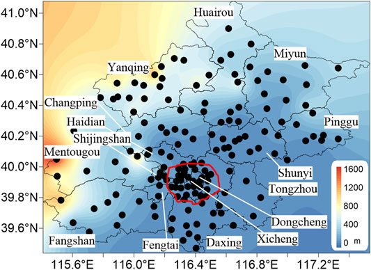
FIGURE 1. The distribution of 16 districts and stations in Beijing. The red line indicates the Fifth Ring Road.

2.2 K-Means Clustering Method and Its Improvements

The K-means algorithm is an unsupervised learning algorithm, which is often applied to the field of data mining [26], and it is a common clustering algorithm. The calculation steps are as follows:

1) The number of samples is N, and k samples are selected randomly as the initial cluster centers.

2) Do calculation of Euclidean distances (D_i,j) from one sample represented with x_i to each clustering center represented with c_j according to Eq. 1. The sample x_i is assigned to the cluster center c_j when the Euclidean distance D_i,J is the shortest. Calculate all the samples like this and assign them to different cluster centers.

3) In order to ensure that the cluster centers can be representative as much as possible, the cluster centers are recalculated by using the samples assigned in different clusters.

4) Repeat steps 2 and 3 until the cluster centers of each sample no longer change.

$D_{i,j}=\left|x_i-c_j\right|,i\in \left[1,N\right],j\in \left[1,k\right],(1)$

$x_i\to c_J,D_{i,J}={\min |}_{j=1}^k{D}_{i,j},i\in \left[1,N\right].(2)$

There are two shortcomings of the K-means method. The first is that the randomness of selecting the initial value results in different results. The method of the ensemble is used in this study. We repeat the clustering several times (the random selection of the initial value), then calculate the ensemble results, and finally determine the clustering results. The second shortcoming is that the selection of the k value directly impacts the clustering results. The optimal number of the samples is related to the structure of the data themselves, but the latter is hard to determine. It is very difficult to determine the optimal solution of the k value. Therefore, the elbow method is used to determine the k value in this study.

2.3 Second Clustering

If the number of samples is too large to be clustered directly, a second clustering method can be used. According to the characteristics of samples, the first clustering is carried out first. Then, the clustering results are used as samples for the second clustering. As shown in Figure 2, the cluster of each station is carried out first, and the second clustering is taken by using the clusters’ results. The distributed clustering can greatly reduce the calculating time and save computing resources. Y_ij (i = 1, 2, 3,..., m; j = 1, 2, 3, ..., n) represents the samples for the first clustering, where m represents a station and n represents moment. C_il (i = 1, 2, 3, ..., m; l = 1, 2, 3, ..., k) represents the first clustering results, and it also represents the samples of second clustering, where k represents the number of first clustering for each station. Pt (t = 1, 2,3, ...,o) represents the clustering result of second clustering.

FIGURE 2

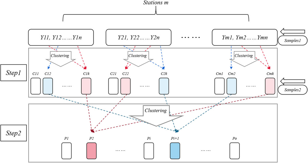
FIGURE 2. The schematic diagram of the two-step clustering analysis.

3 Results and Analyses

3.1 First Clustering: The Number of Clustering

3.1.1 Analyses of the Clustering Results at a Single Station

Taking Shunyi station as an example, we illustrate the process of the K-means clustering. The hourly data during 2008–2017 are taken as samples, and the total number of samples is 87,600. First, the elbow method is used to determine the k value, as shown in Figure 3A. The X-axis represents the k value, and the Y-axis is the average of the Euclidean distance between different samples and their corresponding clusters. It is noted that the average distance is 0 when k = N. In the actual clustering analyses, we hope that k is as small as possible, but the clusters can represent the samples. In Figure 3, with the increase of k, the average distance decreases continuously. When k>10, the average distance is nearly constant. Thus, k is set to 10. Next, the ensemble method is used to minimize the influence of the initial value selection. In this study, the initial values are selected randomly 100 times, and the cluster frequency of each time is shown in Figure 3B with the percentage box line chart. The 10 clusters are marked as C1, C2,…, and C10, respectively. Their average sample proportions are 29.80, 19.01, 12.25, 9.96, 8.56, 6.10, 4.90, 4.14, 3.03, and 2.25%, respectively. However, their variances are small, which means that the clustering of most samples has not changed. For one sample, it may belong to different cluster center. We assign this sample to the cluster center which appears most in 100 clusters. Finally, 10 cluster centers of wind speed at Shunyi station are obtained and shown in Figure 4. Among them, the wind speed cluster of C1 shows the diurnal variation characteristic of “small at night and large in the daytime” with the maximum wind speed around 12:00 CST (China Standard Time; the same below). The wind speed cluster of C2 shows a skewed distribution, with the maximum wind speed in the afternoon. The diurnal variation characteristic of the wind speed cluster of C3 is similar to that of C1, but the wind speed is higher than that of C1. The diurnal variation of C4 is similar to that of C2, but the wind speed is higher than that of C2. The wind speed cluster of C5 is different from other clusters, showing a monotonous increasing diurnal variation. The diurnal variation cluster of C7 is significantly different from that of other clusters, showing a decreasing characteristic. The wind speed of C8 keeps low before 10:00 CST and increases rapidly from 11:00 to 16:00 CST. The wind speed diurnal characteristic of C9 presents the characteristics of linear increasing and linear decreasing. The diurnal variation of wind speed of C10 is similar to that of C6.

FIGURE 3

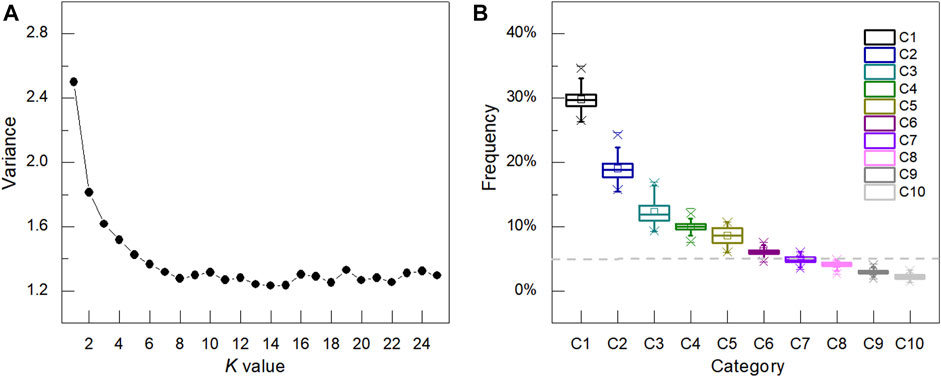
FIGURE 3. (A) The average distance between the sample and the center corresponding to different k values. (B) Percentage box line chart of clustering samples (k = 10).

FIGURE 4

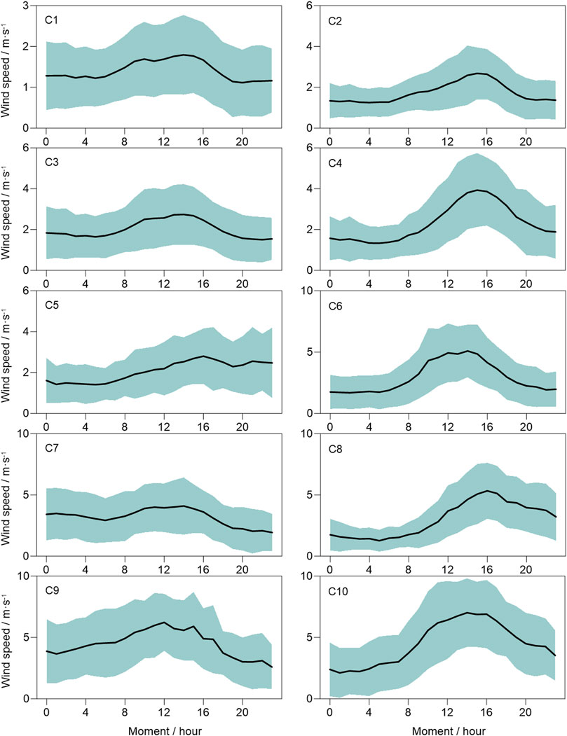
FIGURE 4. The cluster analysis results of the hourly wind speed in 3,650 days at Shunyi station in Beijing. The X-axis is 00:00–23:00 CST, the Y-axis is the wind speed, and C1–C10 represent the 10 clusters, respectively. The black line represents the sample average at different times, and the shade represents one standard deviation of the corresponding sample.

Using the clustering method, we can obtain the typical characteristics of the wind speed diurnal variation. However, the temporal and spatial distributions of the typical characteristics are not clear. Also, the number of the typical characteristics (clusters) that can be obtained at different stations is not clear. Therefore, the observed wind speed data of other 159 stations in Beijing are clustered like those of Shunyi station.

3.1.2 Numbers of the Clusters at Different Stations

The above analyses show that the diurnal variation of the wind speed in Beijing is diverse. The sample numbers of different clusters can be greatly different from those of each other. Thus, typical clusters are analyzed. Cluster analyses are carried out based on the diurnal variations of the wind speed at 160 stations in Beijing. The cluster number (k) is 10. According to Figure 3B, the frequencies of the first few clusters’ samples are larger, which can represent more samples, and these clusters are considered to be typical clusters. In this study, if the sample percentage of one cluster is greater than 5%, the cluster is considered as a typical cluster.

The spatial distribution of the typical cluster number at different stations is shown in Figure 5A. The number of typical clusters in urban and flat areas is less than that of clusters in suburban mountainous areas. There are six stations with four clusters, which are mainly in the suburbs including Shunyi district, Huairou district, and Daxing district, with a low average altitude of 80.83 m (Figure 5B). There are 29 stations with 5 clusters, which are mainly located in the city (including Chaoyang district, Haidian district, Fengtai district, Shijingshan district, Dongcheng district, and Xicheng district) and areas near the city (including Shunyi district, Changping district, and the south of Huairou district). Their average altitude is 113.17 m. There are 79 stations with 6 clusters, which are mainly in the urban area, and the average altitude is 172.85 m. There are 31 stations with 7 clusters. Parts of them are located in the city, and the others are in the area far away from the city, including Miyun district, Pinggu district, and the south of Daxing district. The average altitude is 243.48 m. There are 12 stations with eight and three stations with nine clusters, respectively, which are mainly in the northern area such as Yanqing district, Miyun district, and Pinggu district. The average altitudes are 335.75 and 588.00 m, respectively.

FIGURE 5

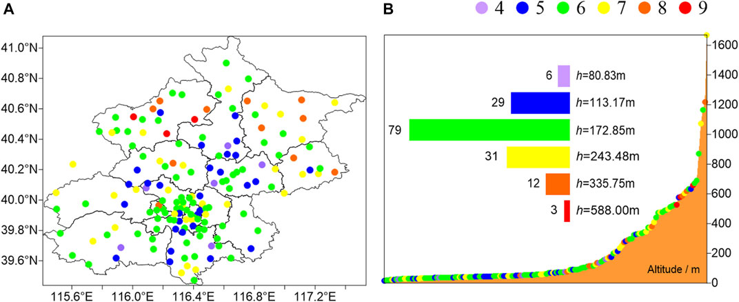
FIGURE 5. (A) Spatial distribution of typical cluster numbers at different stations. (B) Relationship between the typical cluster number and the station altitude. The orange contour represents the station altitude, the scatter chart represents the cluster number of the corresponding station, and the histogram is the number of different clusters and the average altitude of the number. The x-axis represents the stations, and the y-axis represents these stations’ altitude.

In conclusion, the number of clusters with a lower altitude is less, including five clusters in urban areas and seven clusters in the suburb area. In the areas with high altitudes, there are mainly 8 and 9 clusters.

3.1.3 The Interannual Variation of the Cluster Number at Different Stations

The spatial and temporal variations of the typical cluster numbers in different years are further studied. The relationship between the typical cluster number and the station number is shown in Figure 6. During 2008–2012, the station numbers with four clusters (abbreviated to four clusters) and 5 clusters hardly changed. The average station numbers were 6.00 and 30.00, respectively. The station numbers with six to nine clusters were significantly different before and after 2010. The average station numbers during 2008–2010 were 48.00, 41.67, 22.67, and 10.33, respectively. During 2011–2012, the average station numbers were 69.50, 29.50, 15.50, and 4.00, respectively. The stations with 6 clusters increased significantly, while the stations with seven to nine clusters decreased significantly. During 2013–2015, the stations with four to five clusters increased significantly, reaching 20.67 and 53.00, respectively. The stations with six to eight clusters decreased to 44.67, 24.00, and 10.33, respectively. During 2016–2017, the stations with four to five clusters decreased to 16.00 and 37.00, respectively. The stations with six to nine clusters increased. Among them, the station numbers with seven to nine clusters increased significantly by 5.00, 8.17, and 5.50, respectively. Therefore, in the past 10 years, during 2011–2012, the stations with six clusters increased, and during 2013–2015, the stations with four to five clusters increased, which indicates that the clustering numbers at stations in Beijing are decreasing. However, after 2016, the clustering numbers are increasing.

FIGURE 6

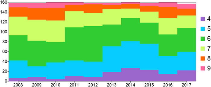
FIGURE 6. Interannual variation characteristics of the total clustering numbers in different years. The x-axis represents time (year), and the y-axis represents the number of stations.

The spatial distribution of the annual cluster numbers is shown in Figure 7. Before 2011, the cluster numbers in Yanqing district, Miyun district, Pinggu district, and Tongzhou district, which are all suburban areas, were mainly seven to nine, while those in the other areas were mainly 5–6. During 2011–2012, the cluster numbers in the urban area, including Yanqing district, and Miyun district changed from 8–9 to 6, while the cluster numbers in the urban area and Shunyi district changed from 7 to 6. During 2013–2015, the cluster numbers in Yanqing district, Huairou district, Fangshan district, and Daxing district, and the urban area changed from 6–7 to 4–5. The variation shows that the number of main clusters was decreasing. While during 2016–2017, the cluster numbers in the urban areas, including Yanqing district, Changping district, and Pinggu district, changed from four to five to six to seven, which means the diurnal variation of wind speed has become more significant. The variation of the cluster numbers in recent years is further studied, as shown in Figure 8. Five to seven clusters remain unchanged before and after the transformation. The annual average station numbers are 17.44, 23.56, and 10.11. The frequency of decreased clusters is 450 after the transformation, that is, 50 stations per year on average. Among them, there are 12.22 stations per year with cluster numbers changing from 6 to 5 and 11.11 stations changing from 7 to 6 per year. The frequency of increased clusters is 400 after the transformation, that is, 44.44 stations per year on average. Among them, 10.11 stations change from 5 to 6, and 9.00 stations change from 6 to 7 per year.

FIGURE 7

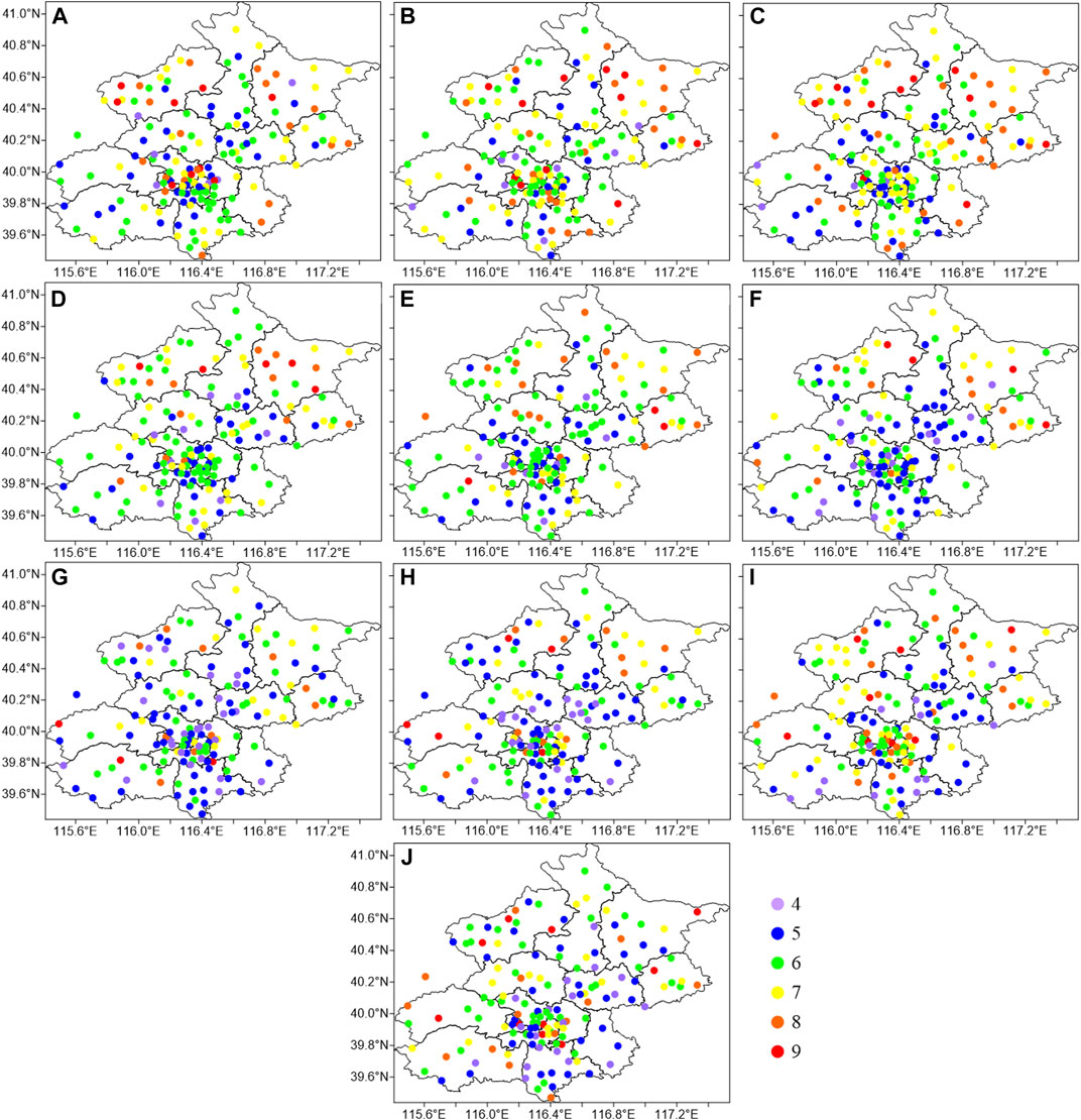
FIGURE 7. Spatial distribution of typical cluster numbers at different stations in different years. (A–J) 2008–2017.

FIGURE 8

FIGURE 8. Transformation of clustering numbers in different years. t represents the cluster number in the current year, and t+1 represents the cluster number in the next year.

In summary, the cluster numbers of the wind speed diurnal variation in different regions of Beijing are significantly different. In urban areas, the cluster numbers are mainly 5 and 6. In the suburbs, the cluster numbers are mainly 7–9. Before 2015, the cluster numbers mainly changed from 7–9 to 4–5. The numbers increased after 2016. In the recent 10 years, the cluster numbers at most stations change from 5 to 6 and from 6 to 7, and the decreasing transformations are more than the increasing ones.

3.2 Second Clustering: Typical Characteristics of the Wind Speed Diurnal Variation

3.2.1 Classification and Diurnal Variation of Different Wind Speeds

The cluster results at different stations are simplified by the second clustering. The cluster results at all stations in Beijing are used as new samples for the second clustering analyses. Figure 9A is the elbow diagram of the second cluster. When the cluster number k is larger than 12, the average distance is almost the same. Therefore, the cluster number is set to 12, and different clusters are marked as P1, P2,…, and P12, respectively. Figure 9B shows the percentage of cumulative days at stations with different clusters. P1–P3 clusters are more than 10%, accounting for 39.85, 21.04, and 11.39%, respectively. The cumulative percentage is 72.28%, representing most of the wind speed diurnal variation. The proportions of P4, P5, and P6 are 9.04, 4.64, and 4.31%, respectively. The days represented by P7–P12 are less than the others, accounting for only 9.73% as shown in Figure 10.

FIGURE 9

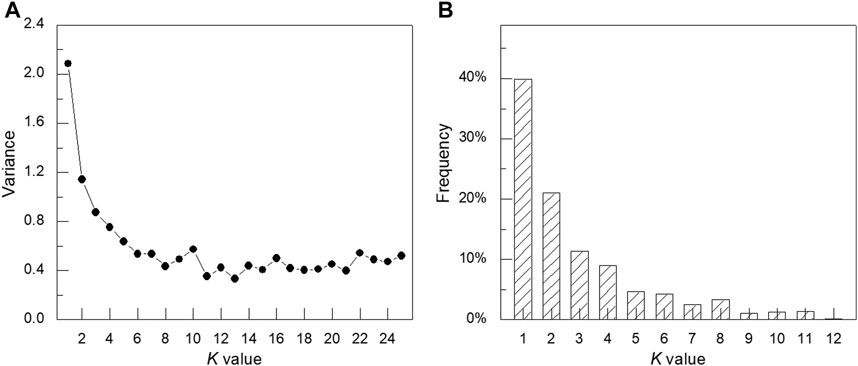
FIGURE 9. (A) Sum of square error of different cluster numbers. (B) Experiments for the cluster number of 10.

FIGURE 10

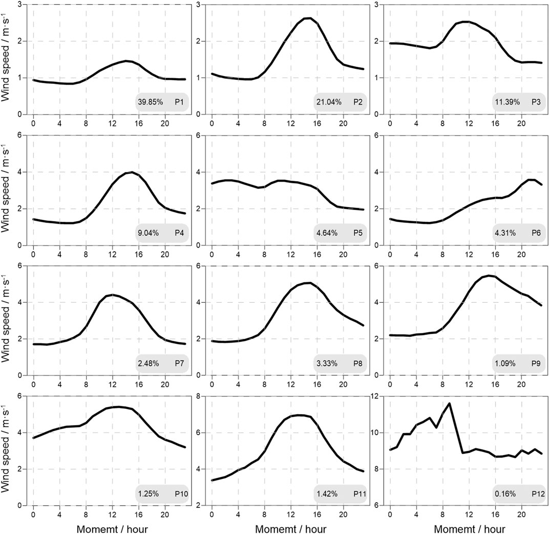
FIGURE 10. Diurnal variation characteristics of different clusters.

The wind speed diurnal variations of different types are shown in Figure 10. The wind speeds of P1–P3 clusters are significantly lower than those of other clusters, and the diurnal average wind speeds are 1.07, 1.56, and 1.95 m s⁻¹, respectively. The wind speed diurnal variation of P1 cluster presents a quasi-symmetric structure, which is in a stable stage (about 1.00 m s⁻¹) during 18:00–08:00 CST and increases during 8:00–14:00 CST. The maximum wind speed is 1.46 m s⁻¹. Then, the wind speed decreases during 14:00–18:00. The wind speed of P2 cluster is asymmetric. The wind speed is almost constant (1.00 m s⁻¹) during 00:00 to 8:00 CST and increases during 08:00–15:00 CST, with a maximum of 2.63 m s⁻¹. The wind speed decreases during 15:00–19:00 CST and decreases slowly during 19:00–23:00 CST. The wind speed of P3 cluster is also distributed asymmetrically. The wind speed is about 2 m s⁻¹ during 00:00–8:00 CST and then increases. The maximum wind speed is at 11:00 and 12:00 CST (both are 2.53 m s⁻¹). Then, the wind speed decreases slowly and remains constant after 19:00 CST (the average wind speed is 1.43 m s⁻¹).

Compared with the average wind speeds of P1–P3 clusters, the average wind speeds of P4–P6 clusters are higher, which are 2.24, 3.03, and 2.14 m s⁻¹, respectively. The wind speed diurnal variation of P4 cluster is similar to that of P2 cluster. The wind speed hardly changes during 00:00–8:00 CST (the average wind speed is 1.31 m s⁻¹), and then increases. The maximum wind speed is at 15:00 CST, which is 3.99 m s⁻¹. The wind speed decreases at 15:00–19:00 CST and becomes constant during 19:00–23:00. The wind speeds of P5 and P6 clusters are monotonous. P5 cluster is a monotonously decreasing type, and P6 is a monotonously increasing type. The wind speed diurnal variation of P7 and P8 is slightly similar to that of P4, but the maximum wind speeds appear at different times. The maximum wind speeds of P7 and P8 clusters occur at 12:00 and 15:00 CST, with the maximum wind speeds of 4.41 and 5.07 m s⁻¹, respectively. Before reaching the maximum wind speed, the wind speed of P9 cluster also keeps constant (the average wind speed is 2.24 m s⁻¹ during 00:00–8:00 CST) at first and then increases. The maximum wind speed of 5.47 m s⁻¹ appears at 15:00 CST. The wind speed decreases rapidly during 15:00–23:00 CST to 3.84 m s⁻¹ at 23:00, which is higher than 2.20 m s⁻¹ at 00:00 CST. The average wind speeds of P10–P12 are significantly higher than those of other clusters, which are 4.39, 5.05, and 9.53 m s⁻¹, respectively. The wind speed of P10 cluster reaches 3.71 m s⁻¹ at 00:00 CST and reaches the maximum value (5.41 m s⁻¹) at 13:00 CST. Then, the wind speed decreases and reaches the minimum value (3.20 m s⁻¹) at 23:00 CST. The wind speed of P11 cluster increases during 00:00–13:00 CST with the maximum of 6.96 m s⁻¹, which decreases during 13:00–23:00 CST. The variation of P12 cluster is different from that of other clusters. The diurnal variation is insignificant. The wind speed shows a linear increasing trend during 00:00–8:00 CST. Then, the wind speed decreases rapidly during 08:00–10:00 CST and nearly remains constant during 11:00–23:00 CST, which is 8.88 m s⁻¹.

To sum up, the diurnal variation of wind speed at all stations in Beijing can be divided into 11 clusters. Except for P5, P6, and P12, the wind speed diurnal variations of other clusters show the characteristics of “large in the daytime and small at night.” However, the different time of the maximum wind speed and the different wind speed lead to multiple clusters of the wind speed diurnal variation of this type. P5 is a monotonic increasing cluster. P6 is a monotonic decreasing cluster. The wind speed of P12 is high without significant diurnal variation.

3.2.2 Interannual Variation and Trend of Different Wind Speed Clusters

Furthermore, the interannual variations of different wind speed cluster frequencies are analyzed, as shown in Figure 11. For P1 cluster, the frequency increases rapidly during 2008–2013, with a trend of 672.54 a⁻¹ (significant at the 98% confidence level, according to the linear trend regression test (LTRT)), which means more and more wind speed is getting smaller. In 2014–2017, the increasing trend stops (the annual average frequency is 2.37 × 10⁴). P1 cluster is mainly distributed in the fifth ring, which might be related to the larger roughness of the city. The frequency of P2 cluster does not increase or decrease significantly in the past 10 years, with an annual average frequency of 1.23 × 10⁴. The frequency of P3 cluster shows a significant negative trend of −105.89 a⁻¹ (significant at the 95% confidence level, according to the LTRT). The frequency of P4 cluster in 2009 (6,062 times) is significantly higher than the annual average (5,193.44 times). After removing this year, there is a significant increasing trend of 42.39 a⁻¹ (significant at the 95% confidence level, according to the LTRT). The frequencies of P5 and P6 significantly decrease with the trends of −87.55 a⁻¹ and −71.99 a⁻¹, respectively (both significant at the 99% confidence level, according to the LTRT). The frequencies of P7–P10 clusters show the variation characteristics of “first decrease and then increase,” with the minimum frequency in 2014. The frequency trends of the four clusters during 2008–2014 are −42.29, −66.39, −28.57, and −49.54 a⁻¹ (all significant at the 98% confidence level, according to the LTRT), respectively. The frequencies of the four clusters increase to varying degrees during 2015–2017. The frequency of P11 is significantly higher in 2010 and during 2015–2017. The frequency of P12 increases significantly during 2015–2017.

FIGURE 11

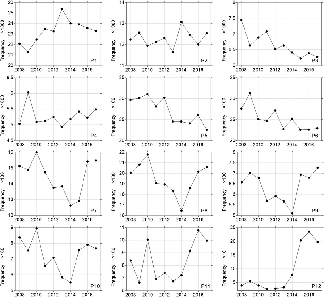
FIGURE 11. Interannual variation of different wind speed clusters (P1–P12). The X-axis represents time, and the Y-axis represents the total frequency (unit: days) of one wind speed cluster at all stations. The coefficient in the figure represents the multiple of the actual data.

In conclusion, there are significant differences in the variation trend of different wind speed clusters in different years. The variation trend of P2 is not significant. P1 and P4 show significant increasing trends. P3, P5, and P6 show significant decreasing trends. The frequencies of P7–P10 decrease before 2014 and then increase. The frequencies of P11 and P12 increase after 2014.

3.2.3 Clusters of Wind Speed at Different Stations

There are regional differences in the frequency of the wind speed clusters at different stations. The frequencies of P1–P12 clusters at each station during 2008–2017 are calculated, as shown in Figure 12. P1 cluster is the most common type. As for the spatial distribution, the frequencies at stations in urban areas are significantly higher than those in suburban areas. There are 25 stations more than 2,400 times. The station number with the frequency more than 1,200 times in the whole area is 81, showing that P1 cluster is the main cluster at most stations. Stations with frequencies less than 800 times are mainly in Yanqing district, Pinggu district, and Fangshan district, and the total number is 12. The stations of P2 cluster with a frequency more than 1,200 times are mainly distributed in Yanqing district, Huairou district, Miyun district, and Pinggu district, and the station number is 24. However, the frequency at most urban stations is less than 400. The stations with high frequencies of P3 cluster are mainly in the suburbs. There are 56 stations with frequencies more than 500 times, which are mainly distributed in Fangshan district, Changping district, Yanqing district, Miyun district, Pinggu district, and Shunyi district. The frequency of P3 cluster in most urban areas is less than 400 times. P4 cluster mainly occurs in the northwest of Beijing, including Mentougou district, Yanqing district, and Changping district. The number of stations with more than 500 times is 26. The frequency of P4 cluster in most urban stations is less than 300. As for P5 cluster, the number of stations with more than 400 times is 17, which are mainly distributed in Yanqing district, Changping district, and Pinggu district. As for P6 cluster, the number of stations with more than 400 times is 12, which are mainly distributed in the urban area and Miyun district. The frequencies of P7 and P8 clusters are low. There are 9 and 10 stations with more than 300 times, respectively, which distribute in the west and northwest of Beijing. There are few stations with P9–P12 clusters. As for P9 cluster, there are seven stations with a frequency of more than 200 times, which are mainly in Changping district, and most of the other stations are less than 100 times. As for P10 cluster, there are nine stations with a frequency of more than 200 times, which are mainly in Changping district and Yanqing district. As for P11 cluster, there are 15 stations with a frequency of more than 200 times, which are mainly distributed in Yanqing district. There are only four stations with P12 cluster. Among them, the frequency at Lingshan station in Mentougou district is 440 times, and the frequency at Foyeding station in Yanqing district is 396 times. At these two stations, the altitudes are 1,669 and 1,217 m, respectively. Therefore, the wind speeds are always high.

FIGURE 12

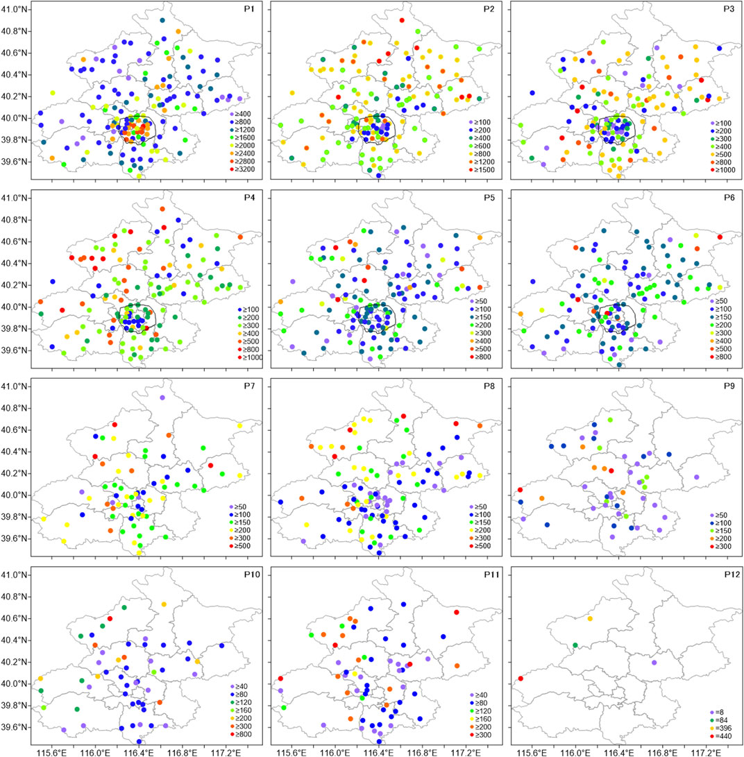
FIGURE 12. Cluster frequency at different stations. The black line is the Fifth Ring Road.

To sum up, there are differences in the main areas of different clusters of wind speed. P1 cluster mainly appears in urban areas. P2 cluster is mainly distributed in urban areas and northern areas. P3 cluster is mainly distributed in the central and northern areas. P4 and P5 clusters are mainly distributed in the northwest. P6 cluster is mainly distributed in the central area.

4 Conclusion and Discussion

In this study, the initial value of the K-means clustering method is selected using an ensemble method. The hourly observation data at 160 observation stations in Beijing in recent 10 years are used for cluster analyses. The different clusters of the wind speed diurnal variation at different stations are studied, and the spatial and temporal variations of the cluster numbers and types at different stations are analyzed. The conclusions are as follows.

1) The cluster analyses are carried out at each station. The wind speed at most stations can be divided into four to nine clusters, and the main clusters are five to seven clusters. There are mainly five to six clusters near the urban area and seven clusters far away from the urban area. The altitudes are high at the stations with 8 and 9 clusters.

2) As for the long-term variation, the number of stations with cluster numbers of four to five increased significantly during 2013–2015, and the number of stations with cluster numbers of six to eight decreased, which means the total number of the wind speed clusters decreased during this period. As for the transformation of cluster numbers in the recent 10 years, the stations with five to six clusters and six to seven clusters tend to transform more than the others, and the transformation to fewer cluster numbers is more than that to more cluster numbers.

3) For all stations, the diurnal variation of the wind speed can be divided into 12 clusters including 9 clusters of “large in the daytime and small at night,” with 1 cluster of monotonous increase, 1 cluster of monotonous decrease, and 1 cluster of strong wind. Among them, nine different clusters of “large in the daytime and small at night” are mainly caused by the different time and value of the maximum wind speed.

4) As for the long-term variation trend, P1 and P4 increase significantly. P3, P5, and P6 decrease. P7–P12 show opposite trends before and after 2014. As for the spatial distribution, P1 cluster is mainly in urban areas, while other types are mainly in suburbs.

The daily variation of wind speed at the station near the urban area is consistent, while in the suburban area, the diurnal variation of wind speed at different stations is quite different, especially for the stations with high altitude. The difference of daily variation of wind speed at more and more stations is small, and the wind speed is small too. Under the background of urbanization, more and more buildings increase the surface roughness, reduce the wind speed, and reduce the difference of daily variation of wind speed at different stations [27]. It is not conducive to the dissipation of urban pollutants and should be paid more attention by the government.

Data Availability Statement

The raw data supporting the conclusions of this article will be made available by the authors, without undue reservation.

Author Contributions

PY and PY contributed to the conception of the study. PY and DZ performed the data analyses and wrote the manuscript. DZ and SL helped preform the analysis with constructive discussions.

Funding

This research has been supported by the Ministry of Science and Technology of China (2018YFA0606302), the Open Project of Key Laboratory of Land Surface Process and Climate Change in Cold and Arid Regions (LPCC2019002), and the National Natural Science Foundation of China (41775078, 42005058, 41675092). The data used in this study can be obtained by contacting the corresponding author: Ping Yang (zz96998@163.com).

Conflict of Interest

The authors declare that the research was conducted in the absence of any commercial or financial relationships that could be construed as a potential conflict of interest.

References

1. Cassiani M, Stohl A, Eckhardt S, Stohl A, Eckhardt S. The Dispersion Characteristics of Air Pollution from the World's Megacities. Atmos Chem Phys (2013) 13:9975–96. doi:10.5194/acp-13-9975-2013

CrossRef Full Text | Google Scholar

2. Li XF, Zhang MJ, Wang SJ, Zhao AF, Ma Q, Zhang MJ, et al. [Variation Characteristics and Influencing Factors of Air Pollution index in China]. Environ. Sci. (2012) 33:1936–43. doi:10.13227/j.hjkx.2012.06.035

PubMed AbstractGoogle Scholar

3. Šinik N, Lončar E. An Estimation of Pollutant Diffusion Rates during Calm Conditions. IL Nuovo Cimento C (1990) 13:917–21. doi:10.1007/bf02514780

CrossRef Full Text | Google Scholar

4. Alan S, Evgeni F. An Analytical Model of an Urban Heat Island Circulation in Calm Conditions. Environ. Fluid Mech. (2019). 19:111–135. doi:10.1007/s10652-018-9621-9

CrossRef Full Text | Google Scholar

5. Yang P, Ren GY, Yan PC, Ren G, Yan P. Evidence for a Strong Association of Short-Duration Intense Rainfall with Urbanization in the Beijing Urban Area. J Clim (2017) 30:5851–70. doi:10.1175/JCLI-D-16-0671.1

CrossRef Full Text | Google Scholar

6. Wang W, Tang DG, Liu HJ, Yue X, Pan Z, Ding Y. Research on Current Pollution Sataus and Pollution Characteristics of PM2.5 in China. Res Environ Sci (2000) 13:1–5. doi:10.3321/j.issn:1001-6929.2000.01.001

Google Scholar

7. Miao L, Liao XN, Wang YC, Liao XN, Wang YC. [Diurnal Variation of PM2.5 Mass Concentration in Beijing and Influence of Meteorological Factors Based on Long Term Date]. Huan Jing Ke Xue (2016) 37(8):2836–46. doi:10.13277/j.hjkx.2016.08.003

PubMed Abstract | CrossRef Full Text | Google Scholar

8. Sun G-Q, Zhang HT, Wang JS, Li J, Wang Y, Li L, et al. Mathematical Modeling and Mechanisms of Pattern Formation in Ecological Systems: a Review. Nonlinear Dyn (2021) 104:1677–96. doi:10.1007/s11071-021-06314-5

CrossRef Full Text | Google Scholar

9. Xue Q, Liu C, Li L, Sun GQ, Liu C, Li L, et al. Interactions of Diffusion and Nonlocal Delay Give Rise to Vegetation Patterns in Semi-arid Environments. Appl Math Comput (2021) 399:126038. doi:10.1016/j.amc.2021.126038

CrossRef Full Text | Google Scholar

10. Makra L, Puskás J, Matyasovszky I, Csépe Z, Lelovics E, Bálint B, et al. Weather Elements, Chemical Air Pollutants and Airborne Pollen Influencing Asthma Emergency Room Visits in Szeged, Hungary: Performance of Two Objective Weather Classifications. Int J Biometeorol (2015) 59:1269–89. doi:10.1007/s00484-014-0938-x

PubMed Abstract | CrossRef Full Text | Google Scholar

11. Forgy EW. Cluster Analysis of Multivariate Data: eIciency versus Interpretability of Classi7cations. Biometrics (1965) 21. doi:10.1080/00207239208710779

CrossRef Full Text | Google Scholar

12. Michael RA. Cluster Analysis for Applications: Probability and Mathematical Statistics. New York: Academic Press (1973). p. 347–53.

13. Li F. Research of the Adaptive Optimization Method about K Value of K-Means Algorithm. Anhui: Anhui University (2015). doi:10.2991/isci-15.2015.29

CrossRef Full Text

14. Yovan AF, Vinay GSS, Akhik G. K-means Cluster Using Rainfall and Storm Prediction in Machine Learning Technique. J Comput Theor Nanoence (2019). 16(8):3265–3269. doi:10.1166/jctn.2019.8174

CrossRef Full Text | Google Scholar

15. Liu KP, Ying ZL, Zhai YK. SAR Image Target Recognition Based on Unsupervised K-Means Feature and Data Augmentation. J Signal Process (2017) 33(3):452–8. doi:10.16798/j.issn.1003-0530.2017.03.029

Google Scholar

16. Kim H-G, Yu YW, Yang Y, Park MH, Yu YW, Yang Y, et al. Portable Environmental Microfluidic Chips with Colorimetric Sensors: Image Recognition and Visualization. Toxicol Environ Health Sci (2019) 11(4):320–6. doi:10.1007/s13530-019-0419-z

CrossRef Full Text | Google Scholar

17. Mao B, Li BC. Building Façade Semantic Segmentation Based on K-Means Classification and Graph Analysis. Arab J Geosci (2019) 12(7):253. doi:10.1007/s12517-019-4431-z

CrossRef Full Text | Google Scholar

18. Salehnia N, Salehnia N, Salehnia N, Ansari H, Kolsoumi S, Bannayan M, et al. Climate Data Clustering Effects on Arid and Semi-arid Rainfed Wheat Yield: a Comparison of Artificial Intelligence and K-Means Approaches. Int J Biometeorol (2019) 63:861–72. doi:10.1007/s00484-019-01699-w

PubMed Abstract | CrossRef Full Text | Google Scholar

19. Mao JL. Text Clustering Algorithm Based on K-Means. Comput Syst Appl (2009) 18(10):85–7. doi:10.3969/j.issn.1003-3254.2009.10.020

Google Scholar

20. Saxena A, Prasad M, Gupta A, Bharill N, Patel OP, Tiwari A, et al. A Review of Clustering Techniques and Developments. Neurocomputing (2017) 267(6):664–81. doi:10.1016/j.neucom.2017.06.053

CrossRef Full Text | Google Scholar

21. Redmond SJ, Heneghan C. A Method for Initialising the K-Means Clustering Algorithm Using Kd-Trees. Pattern Recognition Lett (2007) 28(8):965–73. doi:10.1016/j.patrec.2007.01.001

CrossRef Full Text | Google Scholar

22. Arthur D, Vassilvitskii S. K-Means++: The Advantages of Careful Seeding. Proc Annu Acm-siam Symp Discrete Algorithms (2007) 8:1027–35. doi:10.1145/1283383.1283494

Google Scholar

23. Khan SS, Ahmad A. Cluster center Initialization Algorithm for K-Means Clustering. Pattern Recognition Lett (2004) 25(11):1293–302. doi:10.1016/j.patrec.2004.04.007

CrossRef Full Text | Google Scholar

24. Rodriguez A, Laio A. Clustering by Fast Search and Find of Density Peaks. Science (2014) 344(6191):1492–6. doi:10.1126/science.1242072

PubMed Abstract | CrossRef Full Text | Google Scholar

25. Qiu GY, Zhang J. Adaptive SVM Decision Tree Classification Algorithm Based Om Bisecting K-Means. Appl Res Comput (2012) 29(10):3685–7. doi:10.3969/j.issn.1001-3695.2012.10.021

CrossRef Full Text | Google Scholar

26. Wu GJ, ZhangYuan JLD. Automatically Obtaining K Value Based on K-Means Elbow Method. Comput Eng Softw (2019) 40(5):167–70.

Google Scholar

27. Yang P, Ren GY, Yan PC, Deng JM, Ren G, Yan P, et al. Tempospatial Pattern of Surface Wind Speed and the “Urban Stilling Island” in Beijing City. J Meteorol Res (2020) 34(5):986–96. doi:10.1007/s13351-020-9135-5

CrossRef Full Text | Google Scholar