Detection of Pipeline Deformation Induced by Frost Heave Using OFDR Technology

Introduction

The pipeline network plays an important role in oil and gas transportation. The growing demand for energy supply and the reduction of the world’s oil and gas stocks have led operators to explore and construct new massive pipelines in permafrost such as Russia’s far north [1]. In permafrost or seasonally frozen ground regions, frost heave and thaw settlement can lead to pipeline deformation [2, 3], which is a well-known phenomenon in buried pipelines and can lead to large upward movements of a pipeline. This type of deformation has been understood for a long time and seen in Russia and Canada [4]. The deformation of the pipeline will directly result in the pipeline fracture, causing environmental pollution and even accidents. Monitoring the performance of a pipeline in permafrost terrain is more necessary than that for pipelines installed in temperate areas [5].

Conventionally, pipeline inspection robots with closed-circuit TV [6], which utilize ultrasonic and photogrammetric technology, have been employed as major tools to detect pipeline deformation. However, these methods are not suitable for deformation monitoring in real time. Additionally, the electrical sensors are prone to cause fire and explosion accidents in gas and oil pipelines [7].

Optic fiber sensing technology, with its superior immunity to electromagnetic interference, long-distance transmission, high accuracy, and reliability, is particularly attractive for using in harsh environments and electromagnetic fields. Therefore, fiber optic sensing technology has attracted increasing attention in the study of pipeline deformation monitoring [8, 9]. Using distributed fiber optic sensors, Fabien Ravet et al. [10] presented a solution for pipeline deformation due to ground movement. Deformation such as buckling or pipe deformation was detected by recognizing the abnormal strain distribution along the pipeline. In another case, Fabien Ravet et al. [1] introduced an application of a distributed optic fiber sensor in a gas pipeline in Peru, and several events such as landslides and soil settlement were detected by strain measurement. Dana DuToit et al. [11] conducted a realistic pipeline deformation test, where the fiber optic cables were mounted on the pipe and off the pipe, respectively. Test results showed that both on-pipe and off-pipe fiber optic cables provided valuable magnitude assessment of pipe deformations and strains. Carlos Borda et al. [12] directly attached optic fiber strain cables to pipelines at 3, 9, and 12 o’clock positions, respectively, and used a Brillouin optic time–domain analysis (BOTDA)–based interrogator to record the strain data. By analyzing the continuous strain variation, pipeline deformation and 3D positioning due to geological hazards were monitored. Utilizing the conjugate beam method and BOTDA, Zhang et al [13] conducted a test on a PVC pipe model to reconstruct the deformed shape. It is found that the reconstructed shape of the pipeline model depends on the number of measured points, and the more the measured points, the higher the measuring precision of displacement. For the above studies, pipeline deformation induced by frost heave is not involved. In addition, the distributed strain data provided by BOTDA have a long measurement range, but the spatial resolution and strain accuracy cannot satisfy the requirement of pipeline deformation monitoring very well.

OFDR technology combined with high-performance digital signal processors is used to measure distributed strain with millimeter-scale resolution and microstrain measurement precision [14], providing an effective way for pipeline deformation monitoring. In this paper, OFDR technology was used to monitor the distributed strain and the plane curve reconstruction algorithm was used to calculate the deformed shape from the measured strain. This article aims to provide a new approach for pipeline deformation monitoring in permafrost or seasonally frozen ground regions.

Optic Frequency–Domain Reflectometer–Based Distributed Sensing

The spectral response of the Rayleigh backscatter in an optic fiber will be determined by the effects of strain [15] and temperature [16]. The relationship between the spectrum shift Δv and the variation of strain Δε and temperature Δt is given as

$\Delta v=K_T\Delta t+K_{\epsilon }\Delta \epsilon ,(1)$

where K_T and K_ε are the temperature and strain sensitivity coefficients, respectively. Therefore, the temperature and strain can be measured by detecting the Rayleigh scatter frequency. OFDR technique utilizes swept-wavelength interferometry to measure the Rayleigh backscatter as a function of position in the optic fiber [17]. Figure 1 illustrates the principle of the OFDR. Light from the tunable laser source is split between a measurement arm and a reference arm via an optic fiber coupler. Through the measurement arm, the light is sent to the optic fiber sensor. The backscattered light from the optic fiber sensor returns via the coupler and is combined with the light from the reference arm. After passing through the polarization beam splitter, the combined light will be split into orthogonal states recorded at the S and P detectors. A Fourier transform of these signals yields the phase and amplitude of the signal as a function of length along the sensor [18]. Changes in the local strain and temperature of the optic fiber sensor can be detected by comparing a scan of the sensor in a measurement state to a previously recorded reference scan [19]. Any position of the sensing fiber can be used to measure the strain and temperature, similar to the optic fiber etched with continuous distributed FBG sensors [20]. The detailed introduction of OFDR measurement principles can be seen in the study of Kreger et al. [18].

FIGURE 1

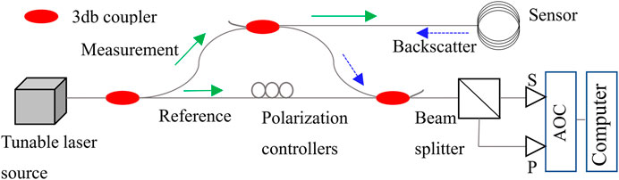
FIGURE 1. Schematic of the OFDR principle.

Theory of Pipeline Shape Monitoring

Curve Reconstruction Algorithm

If a rod is bent, one side is subjected to tensile stresses, while the other side is subjected to compressive stresses. Therefore, there must exist an unstressed surface, which is called the neutral layer. For a rod with a symmetrical cross section, the neutral layer is the surface where the axial line locates at. The curvature of the neutral layer can be used to represent the shape change of a rod. According to Figure 2, the length of the axial line can be expressed as

$L=\theta /k,(2)$

where L is the length of the rod unit; θ is the angle of the arc; and k is the curvature of the rod defined as k = 1/ρ, where ρ denotes the curvature radius of the bent rod. The length variation of the rod surface ΔL is given as

$L+\Delta L=\left(1/k+h/2\right)\theta ,(3)$

where h is the height of the rod unit. The strain ε along the axial direction on the surface of the rod is given as

$\epsilon =\frac{\Delta L}{L}.(4)$

FIGURE 2

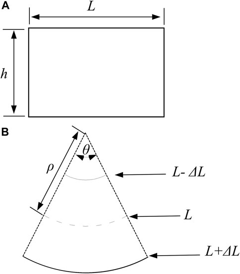
FIGURE 2. Schematic diagram of the rod unit before and after bending. (A) Undeformed unit. (B) Deformed unit.

The relationship between surface strain and curvature can be expressed as

$k=\frac{2\epsilon }{h}.(5)$

Hence, the continuous curvature information can be obtained by the continuous surface strain of the rod.

As shown in Figure 3, O_n and O_n+1 are the two endpoints of the arc; the coordinates of O_n and O_n+1 are (x_n, y_n) and (x_n+1, y_n+1), respectively. If the distance between O_n and O_n+1 is extremely small, the curve segment O_n+1 can be regarded as a microarc ΔS_n. k_n and k_n+1 are the curvature of the arc where O_n and O_n+1 locate at, respectively. α_n and α_n+1 denote the tangential vectors of O_n and O_n+1, respectively. θ_n and θ_n+1 are the angles between the tangent vector of the two points and the x-axis, respectively. l_n is the chord length corresponding to the microarc ΔS_n. Δθ_n denotes the central angle of the microarc ΔS_n. According to Figure 3, the coordinate of O_n+1 can be calculated through O_n. Through iterative calculation, the coordinates of each point are obtained. The equations are given directly as

$\{\begin{array}{l}\Delta \theta ={\theta }_{n+1}-{\theta }_n\\ l_n=2\times \text{sin}\left(\Delta \theta /2\right)/{{\displaystyle k}}_n\\ l_n=\Delta S_n, \left(k_n=0\right)\\ \Delta x_n=l_n\times \text{cos} \left({\theta }_n+\Delta \theta /2\right)\\ \Delta y_n=l_n\times \text{sin} \left({\theta }_n+\Delta \theta /2\right)\\ x_{n+1}=x_n+\Delta x_n\\ y_{n+1}=y_n+\Delta y_n\end{array}(6)$

θ, the key parameter for this curve reconstruction algorithm, can be obtained by solving the differential equation. Based on the definition of curvature, the curvature k of any arc segment can be expressed as

$k\left(s\right)=\frac{d\theta }{ds}(7)$

FIGURE 3

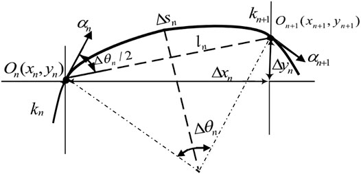
FIGURE 3. Schematic diagram of the curve reconstruction algorithm.

Therefore, θ can be expressed as

$\theta \left(s\right)={\displaystyle \int k\left(s\right)\text{d}s}(8)$

where s denotes the length of the arc. It is assumed that the relationship between curvature and arc length is linear [21]; the curvature k can be given as

$k=A\times s+B,(9)$

where A and B are coefficients.

According to Eqs. 8, 9, θ(s) can be obtained as follows:

$\theta \left(s\right)=A\times s^2/2+B\times s+C(10)$

where C is constant and can be calculated by the deformation boundary conditions of the structure.

The curvature of two adjacent microarcs can be expressed as

$\{\begin{array}{l}{k}_n=A_n\times s_n+B_n\\ k_{n+1}=A_n\times s_{n+1}+B_n\end{array}(11)$

Therefore, A_n and B_n can be obtained by

$\{\begin{array}{l}{A}_n=\left(k_{n+1}-k_n\right)/\left(s_{n+1}-s_n\right)\\ B_n=\left(k_n\times s_{n+1}-k_{n+1}\times s_n\right)/\left(s_{n+1}-s_n\right)\end{array}(12)$

After calculating A, B, and C, θ(s) can be achieved by Eq. 10. Consequently, the curve is reconstructed.

For pipeline shape reconstruction, optic fiber sensors can be attached to the pipeline surface. The curvature k of each arc segment along the pipeline can be calculated by the measured axial strain. The accuracy of the reconstructed shape is related to the measurement accuracy, spatial resolution, and sampling spacing of the measured strain. Since the deformation of the pipeline is continuous, OFDR technology can provide millimeter-scale spatial resolution and sampling spacing. Therefore, the two consecutive measurement points are regarded as a microarc during the calculation, and the coefficients A and B can be calculated by using the curvature k of each measured point. After obtaining θ of each measured point and the corresponding curvature k, the coordinates of each measured point can be calculated in turn using Eq. 6. Consequently, the shape of the pipeline is reconstructed. In practice, optic fiber sensors will be installed on a length that significantly exceeds the area of possible ground movements. Therefore, the segment at the edge of pipeline deformation can be considered fixed and, consequently, the boundary condition for deformed shape calculation. By using the above approach, pipeline deformation monitoring can be realized.

Test Verification

To verify the performance of the curve reconstruction algorithm for pipe structures, a deformation reconstruction test was conducted using a small pipe model. The diameter of the pipe model is 7.7 mm, and the wall thickness is 0.5 mm. The length of the pipe model is 1.2 m. One polyimide-coated optic fiber was bonded on the tensile side of the pipe model to measure the axial strain. An OFDR-based interrogator ODiSI-B from LUNA Innovations was utilized for strain data recording. For the pipe model, the distance between the two support points is 1.0 m. The displacement in the x direction and y direction at both support points was limited, while the rotation was not limited. Concentrated forces were applied to the middle span of the model to produce deformations on the pipe, which were 15 and 25 mm, respectively. In order to verify the accuracy of the plane curve reconstruction algorithm, the deformed shapes of the pipe model were drawn on a graph paper, as shown in Figure 4.

FIGURE 4

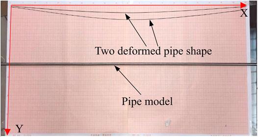
FIGURE 4. Deformation curve of the pipe model subjected to concentrated force.

Figure 5 displays the strain distribution of the pipe model. For the curve reconstruction algorithm, the initial rotation angle of the pipe is set as 0° and the reconstructed shape is tangent to the x-axis. However, the real deformed shape has a certain angle with the x-axis. Therefore, the reconstructed shape should be rotated such that its two ends are placed on the x-axis. Figure 6 shows the reconstructed pipe shapes using the measured strain presented in Figure 5. It is shown that the reconstructed pipe shape and the real deformed shape agree well with each other. Although the strain distribution has fluctuations, it has less influence on the shape reconstruction results. The maximum difference between the calculated value and the real value appears at the midpoint of the pipe model, which is 1.1 and 2.1 mm, respectively. The test results illustrate that the proposed approach can effectively reconstruct the deformed shape of the pipe structure.

FIGURE 5

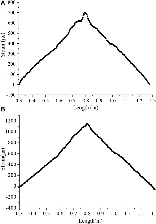
FIGURE 5. Pipe axial strain distribution of the tensile side. (A) Strain distribution of 15 mm deflection. (B) Strain distribution of 25 mm deflection.

FIGURE 6

FIGURE 6. Pipe shape reconstructed by the axial strain distribution. (A) 15 mm deformation. (B) 25 mm deformation.

Pipe Deformation–Monitoring Test

Test Setup

If the temperature of saturated soil falls below freezing, the water will turn into ice, which can result in the volume growth of the saturated soil. Theoretically, the pipe will be bent upward if it is subjected to the force of the expanded saturated soil. Based on this principle, the pipe model was placed in the saturated soil. Both the pipe and the saturated soil were placed in a cold storage to simulate the pipeline deformation.

A steel tank with dimensions of 1.4 × 1.1 × 0.4 m³ was manufactured to contain the saturated soil. There are four angle steels welded together around the steel tank, forming a steel hoop to restrict the deformation of the frost heave in the horizontal direction. The steel hoop is 600 mm away from the tank bottom. On two short sides of the steel tank walls, two round holes with a diameter of 60 mm were fabricated, and the holes are 800 mm away from the bottom.

In the test, the pipe model is a segment of a steel pipe with an outer diameter of 60 mm and a wall thickness of 0.8 mm. To obtain a precise strain distribution, the polyimide-coated fiber was utilized due to its less strain transfer loss. Before bonding the optic fiber, the pipe surface was cleaned by cotton immersed in alcohol. Then, two polyimide-coated fibers were bonded at 0 o’clock and 6 o’clock positions, respectively, using cyanoacrylate adhesive, see Figure 7A. As shown in Figure 7B, 704 silicone rubber glue was used to cover the optic fiber, since it is easily damaged. A temperature compensation sensor was adhered close to the optic fiber at 0 o’clock position. The temperature sensor is a piece of an optic fiber placed into an armored cable. As the optic fiber can freely extend or shrink under the temperature, the strain induced by temperature is measured and deduced from the measured strain. Figure 7C presents the position of the pipe model, and Figure 7D displays the real steel tank filled with saturated soil.

FIGURE 7

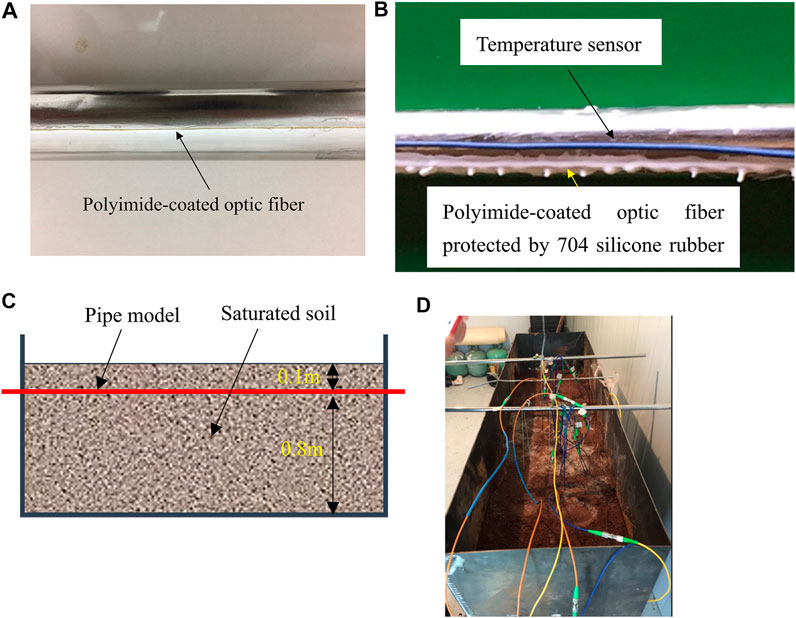
FIGURE 7. Pictures of the test illustration. (A) Polyimide-coated optic fiber sensor. (B) Picture of the strain sensor and temperature sensor. (C) Position of the pipe model. (D) Steel tank.

The pipe model was placed in the steel tank through the two holes. Therefore, the vertical displacement on two ends of the pipe model was restricted when subjected to frost heave force, while the rotation of the two ends was not restricted. The thickness of the overlying soil above the pipe is 10°cm, which is used to simulate the pipeline covered by soil. To provide the freezing condition, the room temperature in the cold storage was decreased from 20 to −23°C and kept at −23°C for 12 h.

Test Results

The strain distribution of the pipe model was recorded every 0.5 h. Figures 8 and 9 display the distributed strain measured by the optic fiber mounted at 6 o’clock and 0 o’clock, respectively. Note that the strain induced by temperature has already been deduced from the distributed strain. The strain data were not all recorded as the interrogator could not detect the sensor signal at certain times. It is shown that the strain measured by the sensor at 6 o’clock position is compressive strain, while the strain measured by the sensor at 0 o’clock is tensile strain. It can be concluded that the pipe has an upward bending due to the frost heave force. And with the increase in the freezing time, the deformation of the pipe constantly increases. After 7 h, the increase is not obvious. It is helpful to directly evaluate the mechanical state of the pipe using strain distribution. As shown in Figures 8 and 9, abnormal strain variations appear in the strain distribution. This is because an iron circle, which was placed at the middle of the pipe, pressed the optic fiber and resulted in the abnormal strain distribution.

FIGURE 8

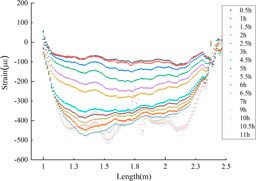
FIGURE 8. Strain distribution measured by the optic fiber at 6 o’clock position.

FIGURE 9

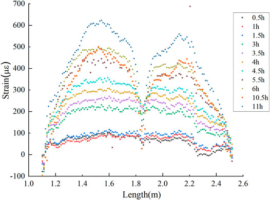
FIGURE 9. Distributed strain measured by the optic fiber at 0 o’clock position.

Using the curve reconstruction algorithm and the distributed strain recorded by a 6 o’clock sensor, the pipe shape at different times was reconstructed and is shown in Figure 10. Note that the measured strain distribution data were directly used to calculate the pipe shape. The abnormal data were not utilized to reconstruct the pipe shape, so Figure 10 only presents the deformed shape before 6 h. It can be seen from Figure 10 that the largest deformation occurs at the midspan position of the pipe. After 6 h of freezing, the maximum deformation is 2.9 mm. From the reconstruction shape of the pipe, it is possible to identify the location with large deformation. The deformation monitoring methods enable people to take preventative measures at an early stage.

FIGURE 10

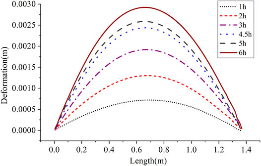
FIGURE 10. Shape reconstructed by the 6 o’clock sensor.

Figure 11 displays the shape reconstructed by a 0 o’clock sensor. Strain data only before 4 h were employed to calculate the pipe shape since the measured strain is interfered by the external environment after 4 h. Comparing the two deformed pipe shapes reconstructed by the two optic fiber sensors, all the maximum deformations of the two test results occur at the middle of the pipe. There are minor differences between these two reconstructed shapes at the same moment. They are 0.7 and 0.5 mm after 1 h, respectively, while after 3 h, the maximum deformations are 1.9 and 1.4 mm, respectively. The differences are probably induced by the fact that the neutral axis is not exactly located at the center of the pipe. The way of directly mounting optic fiber sensors on the pipe may result in an inaccurate reconstructed pipe shape. Besides, the measured strain is easily interfered by the external environment. Therefore, an optic fiber shape sensor, which can overcome the above disadvantages, should be developed in the future study.

FIGURE 11

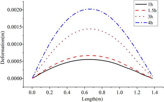
FIGURE 11. Shape reconstructed by the 0 o’clock sensor.

Conclusion

The study of pipe deformation monitoring in the frozen soil area is an important issue. For the shape reconstruction algorithm, the accuracy of the reconstructed shape depends on the number of measured points and sampling spacing. OFDR technology has high accuracy, high spatial resolution, and high sampling spacing in distributed strain measurement. Therefore, we propose to combine the OFDR technology and curve reconstruction algorithm to monitor the pipe deformation. In the experimental study, the OFDR technology and curve reconstruction algorithm are demonstrated to have good performance. However, further studies should be carried out for practical applications, such as to determine how to protect the optic fiber and obtain more precise strain data.

Data Availability Statement

The raw data supporting the conclusion of this article will be made available by the authors, without undue reservation.

Author Contributions

TJ conceived the study, designed the test, and wrote the paper. J-WZ performed the experiments and analyzed the data. YS made constructive comments on the study and participated in paper writing.

Funding

This work was supported by the fund from the National Natural Science Foundation of China (Grant Nos. 52008236 and 61801283) and Shantou University Scientific Research Foundation (Grant No. NFT19039). These grants are greatly appreciated.

Conflict of Interest

The authors declare that the research was conducted in the absence of any commercial or financial relationships that could be construed as a potential conflict of interest.

References

1. Ravet F, Borda C, Rochat E, Niklès M. Geohazard Prevention and Pipeline Deformation Monitoring Using Distributed Optical Fiber Sensing. In: ASME 2013 International Pipeline Geotechnical Conference, July 24–26, 2013, Bogota, Colombia. American Society of Mechanical Engineers Digital Collection (2013).

CrossRef Full Text | Google Scholar

2. Ravet F, Niklès M, Rochat E. A Decade of Pipeline Geotechnical Monitoring Using Distributed Fiber Optic Monitoring Technology. In: ASME 2017 International Pipeline Geotechnical Conference, July 25–26, 2017, Lima, Peru. American Society of Mechanical Engineers Digital Collection (2017).

CrossRef Full Text | Google Scholar

3. Li H, Lai Y, Wang L, Yang X, Jiang N, Li L, et al. Review of the State of the Art: Interactions between a Buried Pipeline and Frozen Soil. Cold regions Sci Technol (2019) 157:171–86. doi:10.1016/j.coldregions.2018.10.014

CrossRef Full Text | Google Scholar

4. Palmer AC, Williams PJ. Frost Heave and Pipeline Upheaval Buckling. Can Geotech J (2003) 40(5):1033–8. doi:10.1139/t03-044

CrossRef Full Text | Google Scholar

5. Oswell JM. Pipelines in Permafrost: Geotechnical Issues and Lessons 12010 R.M. Hardy Address, 63rd Canadian Geotechnical Conference. Can Geotech J (2011) 48(9):1412–31. doi:10.1139/t11-045

CrossRef Full Text | Google Scholar

6. Gomez F, Althoefer K, Seneviratne LD (2003). Modeling of Ultrasound Sensor for Pipe Inspection. In 2003 IEEE International Conference on Robotics and Automation (Cat. No. 03CH37422), September 14–19, 2003, Taipei, Taiwan. IEEE, Vol. 2, pp. 2555–60.

Google Scholar

7. Ren L, Jiang T, Jia ZG, Li DS, Yuan CL, Li HN. Pipeline Corrosion and Leakage Monitoring Based on the Distributed Optical Fiber Sensing Technology. Measurement (2018) 122:57–65. doi:10.1016/j.measurement.2018.03.018

CrossRef Full Text | Google Scholar

8. Ren L, Jiang T, Li DS, Zhang P, Li HN, Song GB. A Method of Pipeline Corrosion Detection Based on Hoop-Strain Monitoring Technology. Struct Control Health Monit (2017) 24(6):e1931. doi:10.1002/stc.1931

CrossRef Full Text | Google Scholar

9. Jiang T, Ren L, Jia ZG., Li DS, Li HN. Pipeline Internal Corrosion Monitoring Based on Distributed Strain Measurement Technique. Struct Control Health Monit (2017) 24(11):e2016. doi:10.1002/stc.2016

CrossRef Full Text | Google Scholar

10. Ravet F, Briffod F, Nikle`s M. Extended Distance Fiber Optic Monitoring for Pipeline Leak and Ground Movement Detection. Int Pipeline Conf (2008) 48579:689–97. doi:10.1115/IPC2008-64521

CrossRef Full Text | Google Scholar

11. DuToit D, Ryan K, Rice J, Bay J, Ravet F. Analysis of Strain Sensor Cable Models and Effective Deployments for Distributed Fiber Optical Geotechnical Monitoring System. In: ASME 2015 International Pipeline Geotechnical Conference, July 15–17, 2015, Bogota, Colombia. American Society of Mechanical Engineers Digital Collection (2015).

CrossRef Full Text | Google Scholar

12. Borda C, Niklès M, Rochat E, Grechanov A, Naumov A, Velikodnev V. Continuous Real-Time Pipeline Deformation, 3D Positioning and Ground Movement Monitoring along the Sakhalin-Khabarovsk-Vladivostok Pipeline. In: International Pipeline Conference, September 24–28, 2012, Calgary, Alberta, Canada. American Society of Mechanical Engineers (ASME) (2012), 45134. p. 179–87. doi:10.1115/IPC2012-90476

CrossRef Full Text | Google Scholar

13. Zhang S, Liu B, He J. Pipeline Deformation Monitoring Using Distributed Fiber Optical Sensor. Measurement (2019) 133:208–13. doi:10.1016/j.measurement.2018.10.021

CrossRef Full Text | Google Scholar

14. Bos J, Klein J, Froggatt M, Sanborn E, Gifford D. Fiber Optic Strain, Temperature and Shape Sensing via OFDR for Ground, Air and Space Applications. In: Nanophotonics and Macrophotonics for Space Environments VII. International Society for Optics and Photonics (2013), 2013, San Diego, CA, 8876. p. 887614. doi:10.1117/12.2025711

CrossRef Full Text | Google Scholar

15. Froggatt M, Moore J. High-spatial-resolution Distributed Strain Measurement in Optical Fiber with Rayleigh Scatter. Appl Opt (1998) 37(10):1735–40. doi:10.1364/AO.37.001735

PubMed Abstract | CrossRef Full Text | Google Scholar

16. Froggatt M, Soller B, Gifford D, Wolfe M. Correlation and Keying of Rayleigh Scatter for Loss and Temperature Sensing in Parallel Optical Networks. In: Optical Fiber Communication Conference, February 22, 2004, Los Angeles, CA. Optical Society of America (2004). p. PD17.

Google Scholar

17. Soller BJ, Wolfe M, Froggatt ME. Polarization Resolved Measurement of Rayleigh Backscatter in Fiber-Optic Components. In: National Fiber Optic Engineers Conference, March 6, 2005, Anaheim, CA. Optical Society of America (2005). p. NWD3.

Google Scholar

18. Kreger ST, Rahim NAA, Garg N, Klute SM, Metrey DR, Beaty N, et al. Optical Frequency Domain Reflectometry: Principles and Applications in Fiber Optic Sensing. In: Fiber Optic Sensors and Applications XIII, 2016, Baltimore, MD. International Society for Optics and Photonics (2016), 9852. p. 98520T.

Google Scholar

19. Galloway KC, Chen Y, Templeton E, Rife B, Godage IS, Barth EJ. Fiber Optic Shape Sensing for Soft Robotics. Soft robotics (2019) 6(5):671–84. doi:10.1089/soro.2018.0131

PubMed Abstract | CrossRef Full Text | Google Scholar

20. Li W, Chen L, Bao X. Compensation of Temperature and Strain Coefficients Due to Local Birefringence Using Optical Frequency Domain Reflectometry. Opt Commun (2013) 311:26–32. doi:10.1016/j.optcom.2013.08.022

CrossRef Full Text | Google Scholar

21. Yi J, Zhu X, Zhang H, Shen L, Qiao X. Spatial Shape Reconstruction Using Orthogonal Fiber Bragg Grating Sensor Array. Mechatronics (2012) 22(6):679–87. doi:10.1016/j.mechatronics.2011.10.005

CrossRef Full Text | Google Scholar