An Attempt to Appreciate Climate Change Impacts From a Rank-Size Rule Perspective

Introduction

All the governments in the world are currently confronted with the difficult problem of both mitigating climate change and maintaining sustainable development. Of the climate change impacts [1–3], in particular, global warming has become the most serious problem necessary to be dealt with urgently in cooperation with the developed and developing countries. In recent years, research articles of climate change have grown substantially in number, even if we restrict our attention within interdisciplinary physics [4–19]. For the analytical methods, besides conventional techniques that have been adopted in statistical physics, novel approaches have been attempted such as wavelet transformation methods [9–13], multiscale entropy analysis [10], convergent cross mapping (CCM) [12], a method using Minkowski distance functions [18], and the vectorial rotation method [19]. In this paper, for representative observational stations in the world as dotted on the map in Figure 1 [19], rank-size analyses are made for vectors that reflect sequential variations of the monthly temperatures and precipitations. The ranking method has been applied principally to revealing a statistical rule or law hidden in texts of natural languages; the most typical example is no doubt the Zipf’s law, being known as a power law relation in the word occurrence versus its rank that is aligned in descending order [20–26]. To our knowledge, however, no attempt has been made to apply the rank-size methodology to the study of climate change impacts. Through specific numerical results we can examine whether, along with conventional applications to complex systems, the rank-size approach is useful for revealing climate change impacts both in the global and in the regional scale.

FIGURE 1

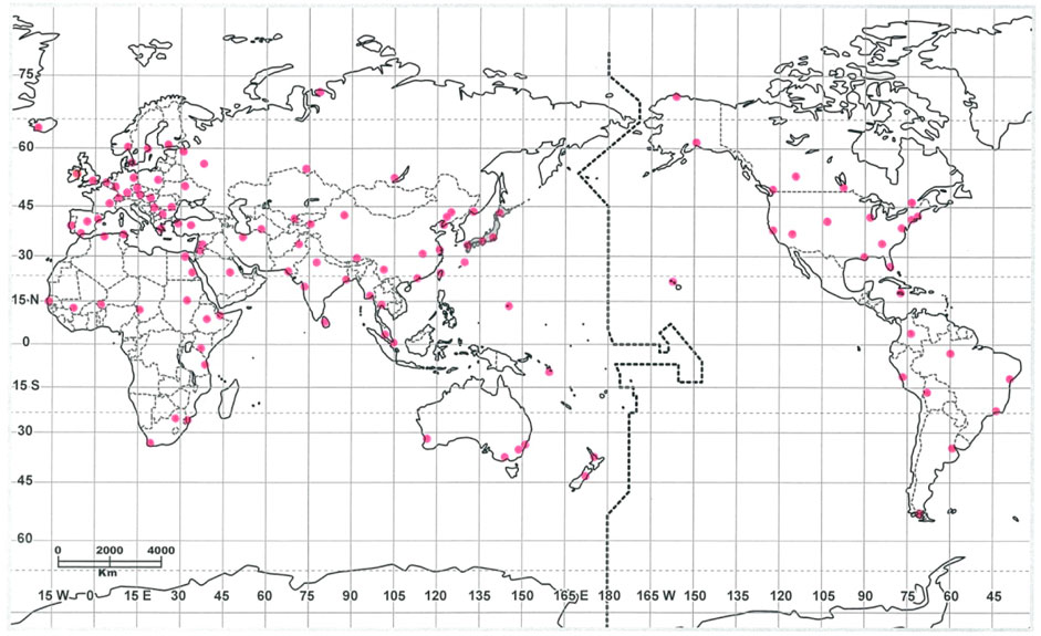
FIGURE 1. The plots of observational stations (pink dots) in the world [19].

Methodology

Generating Angle Data

From the original data of the monthly temperatures and precipitations [27–29], the angle data can be obtained according to the procedure detailed in Ref. [19]. The cross angle θ between two twelve-dimensional vectors, p and q, of the subsequent periods can be obtained by

$\theta =\arccos \left[\left(\mathit{p}\cdot \mathit{q}\right)/\left(\left|\mathit{p}\right|\left|\mathit{q}\right|\right)\right],(1)$

which corresponds to climate change from the former to the latter periods. Here p∙q indicates the scalar product between p and q. For instance, for the temperatures, the magnitude of the angle at a certain station with relatively high latitude increases substantially because of the snow/ice-albedo feedback [30–32].

Rank-Size Analysis

The intersecting angles θ_i (0 ≤θ_i ≤ 180°;i = 1, 2, … , n; n being the size of samples, i.e. the number of stations) will be analyzed statistically. Specifically, as regressions on the angles versus the ranks, three modellings are possible:

$\mathrm{Linear:}\theta =a\mathrm{-}b\chi ,(2)$

$\mathrm{Exponential:}\log \theta =a\mathrm{-}b\chi ,(3)$

$\mathrm{Logarithmic:}\theta =a-b\log \chi ,(4)$

where log abbreviates the common logarithm; χ represents the rank variable in descending order; a and b are positive constants to be determined with the least squares fit. The accuracy of the respective model can be examined by the degree of fit, |r|, namely with the Pearson’s coefficient (0 < |r| < 1), and with the Durbin-Watson ratio, d (0 < d < 4) [33–35]. In what follows, to exclude unnecessary meanderings of dots in the θχ-plane we shall restrict our attention to n less than the Dunbar’s number, i.e., n ≲ 150. Provided that the best logarithmic fit is established, Eq. 4 will subsequently be modified with introducing a positive parameter q [36–38]

${\theta }^q=a-b\log \chi .(5)$

Note that with the additional parameter the optimal values for (a, b) are renewed. Although, mathematically, extending a domain of q to the complex number might be interesting, we confine the domain within the real number. It should be noted here that because the relative angle is confined within [0, 180°], no problem arises in making regression of an angular response variate on a set of linear explanatory variables [39, 40]. In order to analytically examine the behavior of the regression curve, the first derivative of θ is given

$\theta \prime /\theta =-b/\left(q\chi {\theta }^q\right)\propto -1/\left(q{\theta }^q\right),(6)$

where θ’ = dθ/dχ. Eq. 6 shows that for θ > 1, |θ’/θ| gets larger with decreasing q.

Finally, to comprehend the link with the power law (i.e., log-log) relation, with the use of the Box-Cox transformation [41], Eq. 5 will be rewritten as

$\left(\log e\right)\left({\theta }^q-1\right)/q=a\text{'}-b\text{'}\log \chi ,(7)$

$a\text{'}=\left(\log e\right)\left(a-1\right)/q,b\text{'}=\left(\log e\right)b/q,(8)$

where e is the Napier’s constant. In the derivation of Eq. 7 the formula [41]

$\left(\log e\right)\left({\theta }^q-1\right)/q\to \log \theta asq\to 0,(9)$

has been implied. The smaller the magnitude of q, the stronger the kurtosis (i.e., nonlinearities with the positive curvature) in the plane on the rotation angle versus the rank. Thus, along with ΔT (K) and ΔH (mm), by tracing the change of the key parameter q, one can appreciate a sign of a global-scale positive feedback. Here ΔT (K) (ΔH (mm)) stands for the increment of the mean temperature (the mean annual precipitation) from the former to the latter period.

Examples of Rank-Size Rules

To date, sustained efforts have been made to find nontrivial rules in the ranking of a variety of complex systems, not only in linguistics but in geometry, geography, demography, and sciences on social phenomena [20–26, 36–38]. More recently has ranking been regarded as a tool useful for condensing large-scale data that have been accumulating in contemporary sciences such as, e.g., computational metallurgy [42] and gravitational wave astronomy [43], though the results are not yet ready for finding a rule. Below, to illustrate the rank-size rule, three examples of the preceding analysis are selected in Figure 2:

1) The Metropolis of Tokyo with the entire area 2,187 km² consists of 62 municipalities, nine of which are located off the main land [44]. Figure 2A shows the rank dependence of the areas of municipalities (excluding those on islands) in the Metropolis of Tokyo. The line in the figure indicates the optimal fit to Eq. 5 (|r| = 0.9961 with d = 1.861 for q = 0.21 and n = 53). The rank-size rule has been preserved at least for several decades because this prefecture has not experienced a large-scale municipal consolidation. The magnitude of q was found to be smallest among all the prefectures in Japan. Indeed, the value tends to be larger as the number density of municipalities of a prefecture gets lower [36, 37]. In computational geometry, an analog with such an extremely squeezed configuration as seen for Tokyo Metropolis can be found in squared squares [36]. For instance, for the Willcocks’ square [45], q = 0.78 with |r| = 0.9945 and d = 1.450, while for the Duijvestijin’s square [46], q = 0.84 with |r| = 0.9977 and d = 1.521.

2) Japan is divided into 47 prefectures, each of which has been playing a battle to increase its share of the market for the foreign visitors from East Asian countries as well as the United States, Europe, and Australia. Figure 2B plots the rank dependence of the numbers of foreign visitors in the 47 Japanese prefectures (data from January to December, 2016 [47]). The line in the figure indicates the optimal fit (|r| = 0.9988 with d = 1.160 for q = 0.27 and n = 47). With the extremely high degree of fit to the function of Eq. 5 a series of 47 dots align in an exquisite harmony. The top three on the ranking are Tokyo Metropolis, Osaka Prefecture, and Hokkaido. The arrangement of dots on the line bears the strong nonlinearity (q = 0.27), which reminds one of the so-called Matthew effect [48–51] that implies ‘rich-get-richer.’

3) Japanese texts can be written with 45 syllabaries. Figure 2C depicts the dependence of the frequencies of Japanese syllabics in 1,000 male given names [52]. The line in the figure indicates the optimal fit to Eq. 5 (|r| = 0.9977 with d = 2.041 for q = 1.01 and n = 41). It is surprising to note that without interactions among godparents the distribution of the syllabics exhibits such a simple rule. Incidentally it should be remembered here that instead of the power law (Zipf’s law) for the word occurrence, alphabetical frequencies in English texts obey the logarithmic law with q = 1 [20].

FIGURE 2

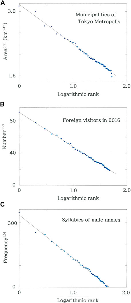
FIGURE 2. Examples of rank-size rules. (A) Rank dependence of the areas of municipalities in the Metropolis of Tokyo. The line indicates the optimized fit (|r| = 0.9961 with d = 1.861 for q = 0.21 and n = 53). (B) Rank dependence of the numbers of foreign visitors in the 47 Japanese prefectures (data from January to December, 2016). The line indicates the optimized fit (|r| = 0.9988 with d = 1.160 for q = 0.27 and n = 47). (C) Rank dependence of the frequencies of Japanese syllabics in 1,000 male given names. The line indicates the optimized fit (|r| = 0.9977 with d = 2.041 for q = 1.01 and n = 41).

Results

Global Analysis

Computed results of the temperatures and precipitations, respectively, are given in Figures 3, 4. In both cases, of the four modellings (Eqs. 2–5) the best fit to the logarithmic function, Eq. 5, has been confirmed. Specifically, for the temperatures, over Period I (from 1931 to 1960) to Period II (from 1951 to 1980), |r| = 0.9974 with d = 0.594 for q = 1.61 (n = 115), while over Period II (from 1951 to 1980) to Period III (from 1981 to 2010), |r| = 0.9961 with d = 0.784 for q = 1.01 (n = 116). For the precipitations, over Period I to II, |r| = 0.9675 with d = 0.409 for q = 1.21 (n = 106), while over Period II to III, |r| = 0.9863 with d = 0.709 for q = 1.51 (n = 107). The reason why the number of dots fluctuates within 106 ≤ n ≤ 116 will be mentioned below. The top-twenty rankings of the rotation angle are listed, respectively, in Tables 1A, 1B, and in Tables 2A, 2B. With these results we comment as follows:

1) For Period I (from 1931 to 1960) to Period II (from 1951 to 1980), rank dependence of the rotation angles of the monthly distributions of temperatures on the World stations is shown in Figure 3A. The line in the figure indicates the optimized fit to Eq. 5 (|r| = 0.9974 with d = 0.594 for q = 1.61 and n = 115), where an exceptional datum on the top ranking, Urumchi, is excluded. It can be seen that the dots are regularly arranged according to the rank-size rule, but there exist three clusters in the dots’ aggregations. The magnitude of q considerably larger than unity (q = 1.61) indicates that the effect due to the snow/ice-albedo feedback is not yet so critical in this period (Table 1A).

2) For Period II (from 1951 to 1980) to Period III (from 1981 to 2010) the rank dependence of the cross angles is given in Figure 3B. The line in the figure indicates the optimal fit with Eq. 5 (|r| = 0.9961 with d = 0.784 for q = 1.01 and n = 116). It is found that although the rank-size rule is preserved, the magnitude of q decreases substantially in comparison with the former period, suggesting that the snow/ice-albedo feedback becomes critical in particular on the highly latitudinal stations in the Northern Hemisphere (for specific numeric, Table 1B).

3) In Figure 3C, scattergram is plotted for rank data of Period II to III versus those of Period I to II (r_S = 0.7907 with d = 2.021 for n = 116). Here r_S denotes the Spearman’s coefficient of rank correlation

$r_S=1-k_n{\sum }_i{\left({\chi }_i-{\Psi }_i\right)}^2,k_n=6/\left[n\left(n^2-1\right)\right](10)$

with the summation Σ_i for i = 1 to n; χ_i and ψ_i are the rank data along the axis of abscissas and ordinates, respectively. It is evident from the plots that, like a stomach bounded by the bottom of an esophagus and the top of a duodenum, the envelope of the intermediate dots swells out, indicating that the ranks exhibit higher mobilities in comparison with those aggregated in the vicinity of the top and bottom.

4) For Period I (from 1931 to 1960) to Period II (from 1951 to 1980), rank dependence of the rotation angles of the monthly distributions of precipitations on the World stations is shown in Figure 4A. The line in the figure indicates the optimized fit with Eq. 5 (|r| = 0.9675 with d = 0.409 for q = 1.21 and n = 106), wherein two exceptional data on the top ranking, Asswan and Kashgar, are foreclosed. First, it is found in the plots that in sharp contrast to the temperature counterpart (|r| = 0.9974 in Figure 3A) the degree of fit, |r|, reduces substantially. Indeed, the arrangement of the dots creates a sigmoid curve rather than a straight line.

5) For Period II (from 1951 to 1980) to Period III (from 1981 to 2010) the rank dependence of the precipitations is given in Figure 4B. The line in the figure indicates the optimal fit to Eq. 5 (|r| = 0.9863 with d = 0.709 for q = 1.51 and n = 107). Aside from the increase of q, there is no substantial change from the result of the former period (Figure 4A). One can see a discontinuity across the rank nine (Urumchi) and ten (Sydney). To conclude, comparison between Figure 4A and Figure 4B indicates that in contrast to the temperatures, there exists no evidence of the climatic positive feedback for the precipitations.

6) In Figure 4C scattergram is plotted for rank data of Period II to III versus the data of Period I to II (r_S = 0.5183 with d = 1.994 for n = 108). In comparison with the temperatures (r_S = 0.7907 for Figure 3C) the rank correlation coefficient reduces substantially. It can be concluded that the reduction in the rank correlation is caused by the stochastic nature of the precipitations.

FIGURE 3

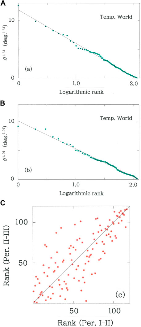
FIGURE 3. Rank dependence of the cross angles of the monthly temperatures on the World stations (Supplementary Tables S1,S2 in Supplementary Material). (A) From Period I (from 1931 to 1960) to Period II (from 1951 to 1980). The line indicates the optimized fit (|r| = 0.9974 with d = 0.594 for q = 1.61 and n = 115). (B) From Period II (from 1951 to 1980) to Period III (from 1981 to 2010). The line in the plots indicates the optimized fit (|r| = 0.9961 with d = 0.784 for q = 1.01 and n = 116). (C) Scattergram of rank data of Period II to III versus the data of Period I to II (r_S = 0.7907 with d = 2.021 for n = 116).

FIGURE 4

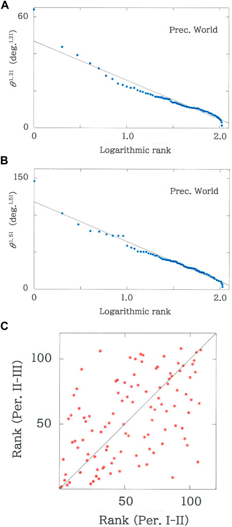
FIGURE 4. Rank dependence of the cross angles of the monthly precipitations on the World stations. (A) From Period I (from 1931 to 1960) to Period II (from 1951 to 1980). The line indicates the optimized fit (|r| = 0.9675 with d = 0.409 for q = 1.21 and n = 106). (B) From Period II (from 1951 to 1980) to Period III (from 1981 to 2010). The line indicates the optimized fit (|r| = 0.9863 with d = 0.709 for q = 1.51 and n = 107). (C) Scattergram of rank data of Period II to III versus the data of Period I to II (r_S = 0.5183 with d = 1.994 for n = 108).

TABLE 1A

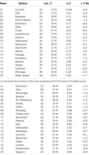
TABLE 1A. Top-twenty World stations in the intersecting angle of the monthly temperatures from Period I (from 1931 to 1960) to Period II (from 1951 to 1980).

TABLE 1B

TABLE 1B. Top-twenty World stations in the intersecting angle of the monthly temperatures from Period II (from 1951 to 1980) to Period III (from 1981 to 2010).

TABLE 2A

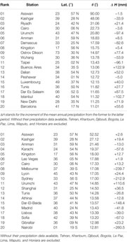
TABLE 2A. Top-twenty World stations in the intersecting angle of the monthly precipitations from Period I (from 1931 to 1960) to Period II (from 1951 to 1980).

TABLE 2B

TABLE 2B. Top-twenty World stations in the intersecting angle of the monthly precipitations from Period II (from 1951 to 1980) to Period III (from 1981 to 2010).

Regional Analysis

Results of the temperatures and precipitations, respectively, are given in Figures 5, 6. In both cases, of the four modellings (Eqs. 2–5) the best fit to the logarithmic function (Eq. 5) has been confirmed. Specifically, for the temperatures, over Period I (from 1931 to 1960) to Period II (from 1951 to 1980), |r| = 0.9973 with d = 0.662 for q = 1.89 (n = 75), while over Period II (from 1951 to 1980) to Period III (from 1981 to 2010), |r| = 0.9883 with d = 0.477 for q = 0.91 (n = 75). For the precipitations, over Period I to II, |r| = 0.9705 with d = 0.666 for q = 3.77 (n = 74), while over Period II to III, |r| = 0.9932 with d = 0.540 for q = 2.49 (n = 75). The reason why the number of dots fluctuates between n = 74 and 75 will be mentioned below. The top-twenty rankings of the rotation angle are listed in Tables 3A, 3B for the temperatures and in Tables 4A, 4B for the precipitations. With these results we remark as follows:

1) For Period I (from 1931 to 1960) to Period II (from 1951 to 1980), rank dependence of the cross angles of the monthly temperatures on the Japanese stations is shown in Figure 5A. The line in the figure indicates the optimized fit to Eq. 5 (|r| = 0.9973 with d = 0.662 for q = 1.89 and n = 75). It can be seen that as has been found in the World counterpart (Figure 3A) the dots are linearly arranged according to the rank-size rule with several clusters in the dots’ aggregations. Again, the magnitude of q becomes considerably larger than unity (q = 1.89), suggesting that the effect arising from the snow/ice-albedo feedback is not yet so apparent in the present period.

2) For Period II (from 1951 to 1980) to Period III (from 1981 to 2010) the rank dependence of the cross angles is given in Figure 5B. The line in the figure indicates the optimized fit to Eq. 5 (|r| = 0.9883 with d = 0.477 for q = 0.91 and n = 75). It is found that although the rank-size rule is preserved, the magnitude of q decreases substantially in comparison with the former period (1.89→0.91), revealing that the snow/ice-albedo feedback becomes critical in particular on the highly latitudinal stations in Japan (for specific numeric, see Table 3B).

3) In Figure 5C, scattergram is plotted for rank data of Period II to III versus those of Period I to II (r_S = 0.6381 with d = 2.125 for n = 75). The dots’ pattern shares a feature with the one in the World temperatures (Figure 3C). Namely, the envelope of the intermediate dots tends to swell out, indicating that except several spots in the vicinity of the top and bottom the ranking shows relatively high mobilities.

4) For Period I (from 1931 to 1960) to Period II (from 1951 to 1980), rank dependence of the rotation angles of the monthly distributions of precipitations on the Japanese stations is shown in Figure 6A. The line in the figure indicates the optimized fit to Eq. 5 (|r| = 0.9705 with d = 0.666 for q = 3.77 and n = 74), wherein an exceptional datum on the top ranking, Karuizawa, is foreclosed. First, it is found in the plots that in contrast to the temperatures (Figure 5A) the degree of fit, |r|, reduces substantially. As has been seen in the World precipitations the arrangement of the dots bears a sigmoid feature rather than a straight one.

5) For Period II (from 1951 to 1980) to Period III (from 1981 to 2010) the rank dependence of the precipitations is given in Figure 6B. The line in the figure indicates the optimized fit to Eq. 5 (|r| = 0.9932 with d = 0.540 for q = 2.49 and n = 75). One can see a discontinuity across the rank four (Obihiro) and five (Owase). Aside from the increase in |r| (0.9705→0.9932) and the decrease in q (3.77→2.49), there is no noticeable change from the result of the former period (Figure 6A). To conclude, comparison between Figure 6A and Figure 6B indicates that in contrast to the temperatures, there exists no evidence of the climatic positive feedback for the precipitations.

6) In Figure 6C scattergram is plotted for rank data of Period II to III versus those of Period I to II (r_S = 0.3797 with d = 1.992 for n = 75). In comparison with the temperatures (r_S = 0.6381 for Figure 5C) the rank correlation coefficient reduces substantially. In the same way as the World precipitations (Figure 4C), this reduction of the rank correlation is attributable to the stochastic nature inherent in the statistics of precipitations.

FIGURE 5

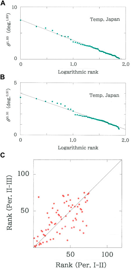
FIGURE 5. Rank dependence of the cross angles of the monthly temperatures on the Japanese stations (Supplementary Table S3 in Supplementary Material). (A) From Period I (from 1931 to 1960) to Period II (from 1951 to 1980). The line indicates the optimized fit (|r| = 0.9973 with d = 0.662 for q = 1.89 and n = 75). (B) From Period II (from 1951 to 1980) to Period III (from 1981 to 2010). The line indicates the optimized fit (|r| = 0.9883 with d = 0.477 for q = 0.91 and n = 75). (C) Scattergram of rank data of Period II to III versus the data of Period I to II (r_S = 0.6381 with d = 2.125 for n = 75).

FIGURE 6

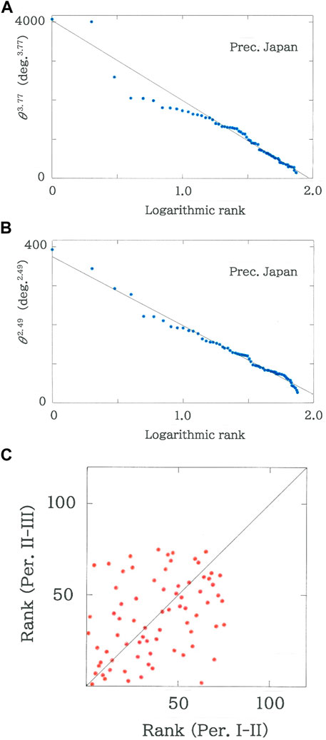
FIGURE 6. Rank dependence of the cross angles of the monthly precipitations on the Japanese stations. (A) From Period I (from 1931 to 1960) to Period II (from 1951 to 1980). The line indicates the optimized fit (|r| = 0.9705 with d = 0.666 for q = 3.77 and n = 74). (B) From Period II (from 1951 to 1980) to Period III (from 1981 to 2010). The line indicates the optimized fit (|r| = 0.9932 with d = 0.540 for q = 2.49 and n = 75). (C) Scattergram of rank data of Period II to III versus the data of Period I to II (r_S = 0.3797 with d = 1.992 for n = 75).

TABLE 3A

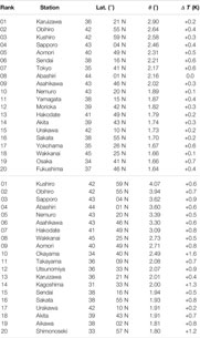
TABLE 3A. Top-twenty Japanese stations in the intersecting angle of the monthly temperatures from Period I (from 1931 to 1960) to Period II (from 1951 to 1980).

TABLE 3B

TABLE 3B. Top-twenty Japanese stations in the intersecting angle of the monthly temperatures from Period II (from 1951 to 1980) to Period III (from 1981 to 2010).

TABLE 4A

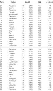
TABLE 4A. Top-twenty Japanese stations in the intersecting angle of the monthly precipitations from Period I (from 1931 to 1960) to Period II (from 1951 to 1980).

TABLE 4B

TABLE 4B. Top-twenty Japanese stations in the intersecting angle of the monthly precipitations from Period II (from 1951 to 1980) to Period III (from 1981 to 2010).

Discussion

Global Analysis

The results of Figure 3 along with Tables 1A, 1B indicate quantitatively that indeed the climate change has arisen in the global scale, but the circumstances are more critical in the northern countries on the Northern Hemisphere than those on the Southern Hemisphere. For the Northern Hemisphere (n = 97) regression analysis of the intersecting angle versus the latitude has shown the typical exponential growth with r = 0.8195 (d = 1.234) for Period II to III, whereas r = 0.7063 (d = 1.754) for Period I to II. For the Southern Hemisphere (n = 19), however, the degree of fit has reduced substantially, i.e., r = 0.5151 (d = 2.113) for Period II to III, while r = 0.5080 (d = 2.708) for Period I to II, though both of them barely maintain the exponentiality. In striking contrast to the temperatures, for the results of the precipitations, no effect arising from the positive feedback has been observed (Figures 4A, B). Instead of the latitudinal dependence, the relations of the rotation angles as a function of the mean annual precipitations on the Entire Sphere (n = 108) have been shown to obey the logarithmic decay as r = −0.7609 (d = 1.332) for Period I to II, and r = −0.6795 (d = 1.611) for Period II to III. Here, as specific data of the annual precipitations, the arithmetic mean of the two subsequent periods has been adopted. The results suggest that a forthcoming large-scale rainmaking or artificial rain project using cloud seeding by spreading silver iodide [53] might make possible arbitrarily (not spontaneously) perturbing the upper ranking in the statistics of World precipitations.

Regional Analysis

For the Japanese stations (n = 75) regression analysis of the intersecting angle versus the latitude has shown the logarithmic growth with r = 0.7361 (d = 1.976) for Period I to II, in contrast to the exponential growth with r = 0.7373 (d = 1.639) for Period II to III. In remarkable contrast to the temperatures, for the results of the precipitations, similarly to the global counterpart, no effect due to the positive feedback has been observed (Figures 6A,B with Table 4A, 4B). Incidentally, for the present, Japan takes no potential interest in the artificial rain project on his territory.

Comparison With Other Methods

The procedure mentioned in Subsection 2.1 can be modified with joining the first differences [19].

$\mathit{p}=\left(<u_1>,<u_2>,\mathrm{...},<u_{12}>;<v_1>,<v_2>,\mathrm{...},<v_{11}>\right),(11)$

$\mathit{q}=\left(<x_1>,<x_2>,\mathrm{...},<x_{12}>;<y_1>,<Y_2>,\mathrm{...},<Y_{11}>\right),(12)$

$<v_j>=<u_{j+1}>-<u_j>,(13)$

$<y_j>=<x_{j+1}>-<x_j>.(14)$

Here j = 1, 2, … , 11. Note that < v_j > and <y_j > stand for the rate of change. To discriminate this method from the original one (i.e., <v_j >≡0 and <y_j >≡0, respectively, in Eqs. 11, 12), we will use the terms, Method A (original; 12 dimensions) and Method B (modified as Eqs. 11, 12; 23 dimensions), respectively. The vectors can be expanded further by adding the second differences [19].

$\mathit{p}=\left(<u_1>,<u_2>,\mathrm{...},<u_{12}>;<v_1>,<v_2>,\mathrm{...},<v_{11}>;<w_1>,<w_2>,\mathrm{...},<w_{10}>\right),(15)$

$\mathit{q}=\left(<x_1>,<x_2>,\mathrm{...},<x_{12}>;<y_1>,<y_2>,\mathrm{...},<y_{11}>;<z_1>,<z_2>,\mathrm{...},<z_{10}>\right),(16)$

$<w_k>=<v_{k+1}>-<v_k>,(17)$

$<z_k>=<y_{k+1}>-<y_k>.(18)$

Here k = 1, 2, … , 10. Note that <w_k> and <z_k> imply the ‘monthly change of curvature.’ To discriminate this method from other methods we will term it Method C (ultimately modified; 33 dimensions).

In Table 5 comparison among these methods is made for optimized fitting parameters in the rank dependence of the rotation angle of the monthly temperatures on the 116 World stations. For Period I to II an exceptional spot, Urumchi, has been excluded. First, one can find, irrespective of the period as well as the method, the high degree of fit is preserved to the function of Eq. 5. For the optimal value of q, however, one can see a significant difference, i.e., the median of the parameter decreases in the subsequent period; this tendency is most remarkable in Method A (q: 1.61→1.01). It is interesting to investigate the results in the data of precipitations. In Table 6 comparison among the three methods is made for optimized fitting parameters in the rank dependence of the intersecting angle of the monthly precipitations on the 108 World stations for which data on precipitations are available. Note that in addition to the eight stations the following spots that include exceptional data have been excluded: for Period I to II, Asswan and Kashgar; for Period II to III, Asswan. In comparison between Table 5 (temperatures versus ranks) and Table 6 (precipitations versus ranks), the degree of fit, |r|, reduces substantially in the latter, indicating that for the ranking of precipitations, there might be a difficulty in adopting the function of Eq. 5. With respect to the change of q, in Table 6 the tendency is reversed, i.e., its value increases in the latter period. The comparative results of the regional analysis are listed in Tables 7 and 8. The principal features that have been confirmed in the global analysis are found to be shared with those in the domestic counterpart. Note that for the temperatures (Table 7), independently of the method, the value of q in Period II to III becomes smaller than unity (q < 1). The blanks in Table 7 have arisen from a certain ill-posed behavior in the prosses of parameter optimization.

TABLE 5

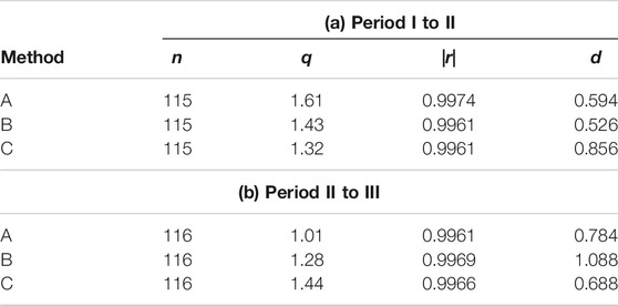
TABLE 5. Comparison of optimal fitting parameters in the rank dependence of the intersecting angle of the monthly temperatures on the World stations. (a) From Period I (from 1931 to 1960) to Period II (from 1951 to 1980); (b) From Period II (from 1951 to 1980) to Period III (from 1981 to 2010).

TABLE 6

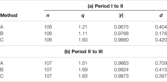
TABLE 6. Comparison of optimal fitting parameters in the rank dependence of the intersecting angle of the monthly precipitations on the World stations. (a) From Period I (from 1931 to 1960) to Period II (from 1951 to 1980); (b) From Period II (from 1951 to 1980) to Period III (from 1981 to 2010).

TABLE 7

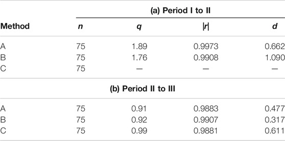
TABLE 7. Comparison of optimal fitting parameters in the rank dependence of the intersecting angle of the monthly temperatures on the Japanese stations. (a) From Period I (from 1931 to 1960) to Period II (from 1951 to 1980); (b) From Period II (from 1951 to 1980) to Period III (from 1981 to 2010).

TABLE 8

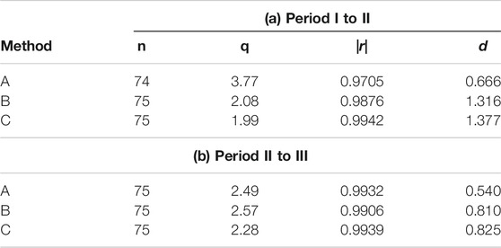
TABLE 8. Comparison of optimal fitting parameters in the rank dependence of the intersecting angle of the monthly precipitations on the Japanese stations. (a) From Period I (from 1931 to 1960) to Period II (from 1951 to 1980); (b) From Period II (from 1951 to 1980) to Period III (from 1981 to 2010).

Conclusion

Independently of the period, the variation of the angles has been found to show a long-tailed decay as a function of their ranks being aligned in descending order. For the temperatures this trend has been shown to get more remarkable in the latter period, confirming that indeed the albedo feedback arises. In contrast to the temperatures (Figure 3 and Table 5), no indication of the feedback has yet been found for the precipitations (Figure 4 and Table 6). To examine the validity of the rank-size analysis in more detail, a regional analysis for 75 stations in Japan has been made as well. Computed results have shown a coherence with the global counterpart. To conclude, through the numerical results of this paper we have confirmed that, along with conventional applications to complex systems, the rank-size approach is useful for revealing climate change impacts not only in the global but in the regional scale. With the current pace in the warming being preserved, the worse (i.e., q = 1.61→q = 1.01→q < 1) for the World temperatures is anticipated for Period III (from 1981 to 2010) to the subsequent Period IV (from 2011 to 2040). The worst scenario will be q→0, in which θ versus χ obeys the power law as suggested in Eqs. 7, 9.

Extension of the methodology to arbitrary circular data in climatic studies [39, 40], such as the wind direction and the animal migration, might be interesting as a future research topic.

Data Availability Statement

The raw data supporting the conclusion of this article will be made available by the authors, without undue reservation.

Author Contributions

The author confirms being the sole contributor of this work and approved it for publication.

Conflict of Interest

The author declares that the research was conducted in the absence of any commercial or financial relationships that could be construed as a potential conflict of interest.

Publisher’s Note

All claims expressed in this article are solely those of the authors and do not necessarily represent those of their affiliated organizations, or those of the publisher, the editors and the reviewers. Any product that may be evaluated in this article, or claim that may be made by its manufacturer, is not guaranteed or endorsed by the publisher.

Supplementary Material

The Supplementary Material for this article can be found online at: https://www.frontiersin.org/articles/10.3389/fphy.2021.687900/full#supplementary-material

References

1.GOSAT Project, the National Institute for Environmental Studies, Japan. A Prompt Report on the Monthly Mean Carbon-Dioxide Concentration Averaged over the Entire Atmosphere (2019). Available at: http://www.gosat.nies.go.jp/recent-global-co2.html (Accessed July 19, 2020).

Google Scholar

2.Metoffice. HadCRU4 Dataset Produced by the Met Office and the Climatic Research Unit at the University of East Anglia. Global Climate In Context As the World Approaches 1 °C Above Pre-Industrial For the First Time (2015). Available at: https://www.metoffice.gov.uk/research/news/2015/global-average-temperature-2015 (Accessed July 19, 2020).

Google Scholar

3.TF Stocker, D Qin, GK Plattner, MMB Tignor, SK Allen, J Boschunget al. editors. Climate Change 2013: The Physical Science Basis (Working Group I Contribution to the Fifth Assessment Report of the Intergovernmental Panel on Climate Change). Cambridge: Cambridge University Press (2014).

Google Scholar

4. Király A, Jánosi IM. Stochastic Modeling of Daily Temperature Fluctuations. Phys Rev E (2002) 65:051102. doi:10.1103/PhysRevE.65.051102

CrossRef Full Text | Google Scholar

5. Lind PG, Mora A, Gallas JA, Haase M. Reducing Stochasticity in the North Atlantic Oscillation Index with Coupled Langevin Equations. Phys Rev E Stat Nonlin Soft Matter Phys (2005) 72:056706. doi:10.1103/PhysRevE.72.056706

PubMed Abstract | CrossRef Full Text | Google Scholar

6. Redner S, Petersen MR. Role of Global Warming on the Statistics of Record-Breaking Temperatures. Phys Rev E Stat Nonlin Soft Matter Phys (2006) 74:061114. doi:10.1103/PhysRevE.74.061114

PubMed Abstract | CrossRef Full Text | Google Scholar

7. Verdes PF. Global Warming Is Driven by Anthropogenic Emissions: A Time Series Analysis Approach. Phys Rev Lett (2007) 99:048501. doi:10.1103/PhysRevLett.99.048501

PubMed Abstract | CrossRef Full Text | Google Scholar

8. Newman WI, Malamud BD, Turcotte DL. Statistical Properties of Record-Breaking Temperatures. Phys Rev E Stat Nonlin Soft Matter Phys (2010) 82:066111. doi:10.1103/PhysRevE.82.066111

PubMed Abstract | CrossRef Full Text | Google Scholar

9. Rossi A, Massei N, Laignel B. A Synthesis of the Time-Scale Variability of Commonly Used Climate Indices Using Continuous Wavelet Transform. Glob Planet Change (2011) 78:1–13. doi:10.1016/j.gloplacha.2011.04.008

CrossRef Full Text | Google Scholar

10. Balzter H, Tate N, Kaduk J, Harper D, Page S, Morrison R, et al. Multi-Scale Entropy Analysis as a Method for Time-Series Analysis of Climate Data. Climate (2015) 3:227–40. doi:10.3390/cli3010227

CrossRef Full Text | Google Scholar

11. Tamazian A, Ludescher J, Bunde A. Significance of Trends in Long-Term Correlated Records. Phys Rev E Stat Nonlin Soft Matter Phys (2015) 91:032806. doi:10.1103/PhysRevE.91.032806

PubMed Abstract | CrossRef Full Text | Google Scholar

12. Huang X, Hassani H, Ghodsi M, Mukherjee Z, Gupta R. Do Trend Extraction Approaches Affect Causality Detection in Climate Change Studies. Physica A: Stat Mech its Appl (2017) 469:604–24. doi:10.1016/j.physa.2016.11.072

CrossRef Full Text | Google Scholar

13. Zhang F, Yang P, Fraedrich K, Zhou X, Wang G, Li J. Reconstruction of Driving Forces from Nonstationary Time Series Including Stationary Regions and Application to Climate Change. Physica A: Stat Mech its Appl (2017) 473:337–43. doi:10.1016/j.physa.2016.12.088

CrossRef Full Text | Google Scholar

14. Matcharashvili T, Zhukova N, Chelidze T, Founda D, Gerasopoulos E. Analysis of Long-Term Variation of the Annual Number of Warmer and Colder Days Using Mahalanobis Distance Metrics - A Case Study for Athens. Physica A: Stat Mech its Appl (2017) 487:22–31. doi:10.1016/j.physa.2017.05.065

CrossRef Full Text | Google Scholar

15. Moon W, Agarwal S, Wettlaufer JS. Intrinsic Pink-Noise Multidecadal Global Climate Dynamics Mode. Phys Rev Lett (2018) 121:108701. doi:10.1103/physrevlett.121.108701

PubMed Abstract | CrossRef Full Text | Google Scholar

16. Hassani H, Silva ES, Gupta R, Das S. Predicting Global Temperature Anomaly: A Definitive Investigation Using an Ensemble of Twelve Competing Forecasting Models. Physica A: Stat Mech its Appl (2018) 509:121–39. doi:10.1016/j.physa.2018.05.147

CrossRef Full Text | Google Scholar

17. Wang C, Wang ZH, Sun L. Early-Warning Signals for Critical Temperature Transitions. Geophys Res Lett (2020) 47:e2020GL088503. doi:10.1029/2020gl088503

CrossRef Full Text | Google Scholar

18. Wang C, Wang Z-H, Li Q. Emergence of Urban Clustering Among U.S. Cities under Environmental Stressors. Sustain Cities Soc (2020) 63:102481. doi:10.1016/j.scs.2020.102481

CrossRef Full Text | Google Scholar

19. Hayata K. Global-Scale Synchronization in the Meteorological Data: A Vectorial Analysis That Includes Higher-Order Differences. Climate (2020) 8:128. doi:10.3390/cli8110128

CrossRef Full Text | Google Scholar

20. Kanter I, Kessler DA. Markov Processes: Linguistics and Zipf's Law. Phys Rev Lett (1995) 74:4559–62. doi:10.1103/physrevlett.74.4559

PubMed Abstract | CrossRef Full Text | Google Scholar

21. Yang AC-C, Hseu S-S, Yien H-W, Goldberger AL, Peng C-K. Linguistic Analysis of the Human Heartbeat Using Frequency and Rank Order Statistics. Phys Rev Lett (2003) 90:108103. doi:10.1103/physrevlett.90.108103

PubMed Abstract | CrossRef Full Text | Google Scholar

22. Alvarez-Martinez R, Martinez-Mekler G, Cocho G. Order-Disorder Transition in Conflicting Dynamics Leading to Rank-Frequency Generalized Beta Distributions. Physica A: Stat Mech its Appl (2011) 390:120–30. doi:10.1016/j.physa.2010.07.037

CrossRef Full Text | Google Scholar

23. Blumm N, Ghoshal G, Forró Z, Schich M, Bianconi G, Bouchaud J-P, et al. Dynamics of Ranking Processes in Complex Systems. Phys Rev Lett (2012) 109:128701. doi:10.1103/physrevlett.109.128701

PubMed Abstract | CrossRef Full Text | Google Scholar

24. Ausloos M. Hint of a Universal Law for the Financial Gains of Competitive Sport Teams. The Case of Tour de France Cycle Race. Front Phys (2017) 5:59. doi:10.3389/fphy.2017.00059

CrossRef Full Text | Google Scholar

25. Morales JA, Colman E, Sánchez S, Sánchez-Puig F, Pineda C, Iñiguez G, et al. Rank Dynamics of Word Usage at Multiple Scales. Front Phys (2018) 6:45. doi:10.3389/fphy.2018.00045

CrossRef Full Text | Google Scholar

26. Mehri A, Agahi H, Mehri-Dehnavi H. A Novel Word Ranking Method Based on Distorted Entropy. Physica A: Stat Mech its Appl (2019) 521:484–92. doi:10.1016/j.physa.2019.01.080

CrossRef Full Text | Google Scholar

27.The National Astronomical Observatory of Japan. Chronological Scientific Tables, Vol. 59. Tokyo: Maruzen (1985).

Google Scholar

28.The National Astronomical Observatory of Japan. Chronological Scientific Tables, Vol. 66. Tokyo: Maruzen (1992).

Google Scholar

29.The National Astronomical Observatory of Japan. Chronological Scientific Tables, Vol. 91. Tokyo: Maruzen (2017).

Google Scholar

30. Weart SR. The Discovery of Global Warming. Cambridge, MA: Harvard University Press (2008).

Google Scholar

31. Berger JJ. Climate Peril. Berkeley, CA: Northbrae (2014).

Google Scholar

32. Wadhams P. A Farewell to Ice: A Report from the Arctic. London: Penguin Books (2016).

Google Scholar

33. von Storch H, Zwiers FW. Statistical Analysis in Climate Research. Cambridge: Cambridge University Press (2000).

Google Scholar

34.H von Storch, and A Navarra, editors. Analysis of Climate Variability: Applications of Statistical Techniques. 2nd ed. Berlin: Springer (2010).

Google Scholar

35. Chatterjee S, Hadi AS. Regression Analysis by Example. 5th ed. Hoboken, NJ: Wiley (2012).

Google Scholar

36. Hayata K. Statistical Properties of Extremely Squeezed Configurations: A Feature in Common between Squared Squares and Neighboring Cities. J Phys Soc Jpn (2003) 72:2114–7. doi:10.1143/jpsj.72.2114

CrossRef Full Text | Google Scholar

37. Hayata K. A Time-Dependent Statistical Analysis of the Large-Scale Municipal Consolidation. Forma (2010) 25:37–44.

Google Scholar

38. Hayata K. Phonological Complexity in the Japanese Short Poetry: Coexistence between Nearest-Neighbor Correlations and Far-Reaching Anticorrelations. Front Phys (2018) 6:31. doi:10.3389/fphy.2018.00031

CrossRef Full Text | Google Scholar

39. Fisher NI, Lee AJ. Regression Models for an Angular Response. Biometrics (1992) 48:665–77. doi:10.2307/2532334

CrossRef Full Text | Google Scholar

40. Jammalamadaka SR, SenGupta A. Topics in Circular Statistics. Singapore: World Scientific (2001).

Google Scholar

41. Vélez JI, Correa JC, Marmolejo-Ramos F. A New Approach to the Box-Cox Transformation. Front Appl Math Stat (2015) 1:12. doi:10.3389/fams.2015.00012

CrossRef Full Text | Google Scholar

42. Lejaeghere K, Cottenier S, Van Speybroeck V. Ranking the Stars: A Refined Pareto Approach to Computational Materials Design. Phys Rev Lett (2013) 111:075501. doi:10.1103/PhysRevLett.111.075501

PubMed Abstract | CrossRef Full Text | Google Scholar

43. Kim K, Li TGF, Lo RKL, Sachdev S, Yuen RSH. Ranking Candidate Signals with Machine Learning in Low-Latency Searches for Gravitational Waves from Compact Binary Mergers. Phys Rev D (2020) 101:083006. doi:10.1103/physrevd.101.083006

CrossRef Full Text | Google Scholar

44.Tsuneta Yano Commemorative Association. Kensei: The Data Book for the 47 Prefectures in Japan. Tokyo: Tsuneta Yano Commemorative Association (2017).

Google Scholar

45. Federico PJ. Squaring Rectangles and Squares. In: JA Bondy, and USR Murty, editors. Graph Theory and Related Topics. New York, NY: Academic Press (1979). p. 173–96.

Google Scholar

46. Duijvestijn AJW. Simple Perfect Squared Square of Lowest Order. J Comb Theor Ser B (1978) 25:240–3. doi:10.1016/0095-8956(78)90041-2

CrossRef Full Text | Google Scholar

47.The Japan Tourist Agency, the Ministry of Land, Infrastructure and Transport. Statistical Survey on Foreign Visitors (2017). Available at: https//www.mlit.go.jp/common/001190401.pdf (Accessed March 23, 2021).

Google Scholar

48. Merton RK. The Matthew Effect in Science. Science (1968) 159:56–63. doi:10.1126/science.159.3810.56

PubMed Abstract | CrossRef Full Text | Google Scholar

49. Price DDS. A General Theory of Bibliometric and Other Cumulative Advantage Processes. J Am Soc Inf Sci (1976) 27:292–306. doi:10.1002/asi.4630270505

CrossRef Full Text | Google Scholar

50. Barabási A-L, Albert R. Emergence of Scaling in Random Networks. Science (1999) 286:509–12. doi:10.1126/science.286.5439.509

PubMed Abstract | CrossRef Full Text | Google Scholar

51. Érdi P. Ranking. New York, NY: Oxford University Press (2020).

Google Scholar

52. Nishizawa N, Makino K. Ranking of Japanese Given Names. Tokyo: Shinjimbutsuoraisha (2001).

Google Scholar

53. Bostock B. China Is Massively Expanding its Weather-Modification Program, Saying It Will Be Able to Cover Half the Country in Artificial Rain and Snow by 2025 (2021). Available at: https://www.businessinsider.jp/post-225599 (Accessed March 23, 2021).

Google Scholar