Improved Smart Pseudoscopic-to-Orthoscopic Conversion Algorithm for Integral Imaging With Pixel Information Averaging

Introduction

Three-dimensional display [1] has been continuously developed since its appearance, and integral imaging (InI) is a very promising three-dimensional display technology. In 1908, Lippmann first proposed integral photography (IP) [2], which was later called InI. The emergence of InI provides a possible way for three-dimensional display, which has attracted the attention of many scientific researchers. InI is generally divided into two systems: capture and display. It uses a pinhole array (PA), lens array (LA), or camera array to sample objects in the capture system and then reproduces the objects in the display system. Compared with the two-dimensional display, it retains the depth information of the objects and essentially uses discrete light field sampling to approximate the continuous light field in reality. In 2018, Corral and Javidi [3] reviewed recent advances in 3D imaging and mainly introduced the principles and application of InI, which facilitated people’s understanding and analysis of InI capture and display systems. In this paper, we will report the average SPOC algorithm, which can generate new EIAs more accurately.

Numerous studies have shown that the loaded EIA has an important influence on the imaging quality. In addition, as shown in Figure 1, during the InI display process, the depth information of the reproduced object will be reversed, which is called the artifact problem. The artifact problem is an inherent problem of InI. In 1931, Ives [4] tried to overcome this problem for the first time and proposed a two-step recording method. He used the reconstructed image as the object to record the second set of elemental images (EIs). In 1967, Chutjian et al. [5] overcame the artifact problem when dealing with computer-generated three-dimensional objects, which can form an orthoscopic image in a single recording process. In 1997, Okano et al. [6] proposed to use standard devices to capture EIs; then, each EI is rotated 180° around its center, but the image reconstructed by this method is a virtual image. In 2001, Erdmann et al. [7] solved the artifact problem electronically and achieved high-resolution three-dimensional display by using a moving microlens array and a low-resolution camera. In 2003, Jang et al. [8] used a condenser to record the EIs in which the object’s depth information is inversed during the capture process, and the EIs are also rotated by 180° in the display process. However, the reconstructed image under this scheme often shows obvious distortion. In 2005, Corral et al. [9] proposed the smart pixel mapping (SPM) algorithm. The important idea is to use the digital method for the optical reproduction of the first step and the optical recording of the second step in the two-step method of Ives. In 2007, Park et al. [10, 11] converted the directional scene into two-dimensional images and reconstructed it into a new EIA through segmentation and shearing. In 2008, Shin et al. [12] proposed a computational integral imaging reconstruction (CIIR) method based on the SPM algorithm, which can effectively improve the resolution of the reconstructed plane images. In 2014, Zhang et al. [13] used negative refractive index materials to achieve one-step InI and avoided the problem of resolution reduction inherent to the optical or digital two-step methods. In 2015, Yu et al. [14] eliminated the artifact problem by obtaining precise depth information and achieved smooth motion parallax. In the same year, Chen et al. [15] proposed the multiple elemental image mapping (MEIM) method, which can enhance the resolution of the generated orthographic view image. In 2018, Wang et al. [16] analyzed the problems in the SPM algorithm and proposed a fast-direct pixel mapping algorithm that can adapt to different display parameters. In 2020, Zhang et al. [17] used a transmissive mirror device and a light filter to eliminate pseudoscopic issue, which can present a high-quality 3D image.

FIGURE 1

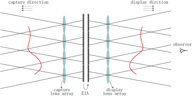
FIGURE 1. Artifacts in integral imaging.

In 2010, Navarro et al. [18] proposed the SPOC algorithm, which is currently the most widely used method to solve the artifact problem. The algorithm establishes the mapping relationship between the display pixels and the synthetic pixels by setting a reference plane, which can solve the problem of depth inversion and synthesize a new EIA using the already captured EIA so as to apply to the display system with different parameters. Subsequently, the team used the SPOC algorithm to achieve head-tracking three-dimensional InI [19], which can realize the viewing of the three-dimensional scene with the head rotated. In 2014, Corral et al. [20] improved the SPOC algorithm. By cropping EIs, the field of view (FOV) and reference plane can be adjusted to produce a three-dimensional display with full parallax. In 2015, Xiao et al. [21] proposed to establish multiple reference planes based on depth information estimation, thereby reducing the pixel mapping error of the deep scene in the process of synthesizing the new EIA. In 2018, Yan et al. [22] applied the LA shift technology to the SPOC algorithm and generated accurate EIs by freely selecting the reference plane, thus realizing the correct pixel mapping of objects with large depth information. In the same year, Yang et al. [23] also paid attention to this research and proposed to use off-axis acquisition to realize light field display, which improves the efficiency of real-time data processing. In 2021, Yan et al. [24] proposed an EIA generation method using pixel fusion based on the SPOC algorithm and obtained good results.

The SPOC algorithm is simple and practical, but it also has disadvantages. It equates the synthetic LA to a PA. Obviously, compared to the pinhole, the synthetic lens has a converging effect on the rays passing through it, which is not reflected here. In addition, it uses only one simulated ray to find the display pixel corresponding to the display lens that the ray intersects, ignoring the contribution of other display lenses to the synthetic pixel. In fact, there are gaps between pixels. When the ray intersects the gaps, the SPOC algorithm will cause the matching error between the display pixels and the synthetic pixels. In addition, due to mechanical errors or operating errors, the display pixels in some EIs may have large errors or are even empty pixels, and then the synthetic pixels we get will also have large errors or are even empty pixels. In this paper, we improve the SPOC algorithm and propose a new EIA generation algorithm based on the average of pixel information—the average SPOC algorithm, which fully considers the converging effect of the synthetic lens on the rays and reduces the pixel-matching errors, mechanical errors, and man-made errors in the SPOC algorithm. In real scenes, due to factors such as occlusion and lighting, the pixels of the pictures we get at some viewing angles may have large errors and are even empty pixels. In this case, the SEIA generated by the average SPOC algorithm will be more accurate and the reconstruction effect is better.

To clarify the average SPOC algorithm, this paper is organized as follows. Principle and Problems of the Smart Pseudoscopic-to-Orthoscopic Conversion Algorithm explains the principle and problems of the SPOC algorithm. In Principles of the Smart Pseudoscopic-to-Orthoscopic Conversion 1 Algorithm and the Average Smart Pseudoscopic-to-Orthoscopic Conversion Algorithm, we propose the SPOC1 algorithm, which is the transition of the average SPOC algorithm. Then, we revise the SPOC1 algorithm and propose the average SPOC algorithm. In Experimental Verification and Discussion, experiments are conducted and detailed discussion is made to verify the superiority of the average SPOC algorithm. Finally, Conclusion reviews the research and makes a summary of our work.

Principle and Problems of the Smart Pseudoscopic-to-Orthoscopic Conversion Algorithm

The principle of the SPOC algorithm is shown in Figure 2. The left side is the display end, and the right side is the synthetic end. The pitch, $p_D$, the focal length, $f_D$, of the display lens, and the gap, $g_D$, from the display LA plane to the display EIA plane are the same as those in the previous capture system, which also means that the display system can reuse the previous acquisition system. In the simulated display, the already captured EIA is used as the display EIA. The synthetic LA is equivalent to a PA. The length of each synthetic elemental image (SEI) is equal to the pitch of the synthetic lens, which are both $p_S$. The gap from the synthetic LA plane to the SEIA plane is $g_S$, and the distance from the display LA plane to the synthetic LA plane is $D$. Select the reference plane; the distance from it to the display LA plane is $d_D$, and the distance from it to the synthetic LA plane is $d_S$. According to the principle of reversibility of the ray path, the simulated ray starts from the center of the $t^{th}$ pixel of the $j^{th}$ SEI, which the $x$ coordinate corresponding to the center of the t-th pixel of the j-th SEI is $x_S$, and passes through the corresponding PA. Then, we can get the $x$ coordinate of the point where the ray intersects the reference plane, ${\Delta }_O$, and the $x$ coordinate of the point where the ray intersects the display lens, $\Delta D$. Thus, the index of the display lens, $u$, can be calculated as

$u=Ceil\left[\frac{\Delta D}{p_D}\right].(1)$

FIGURE 2

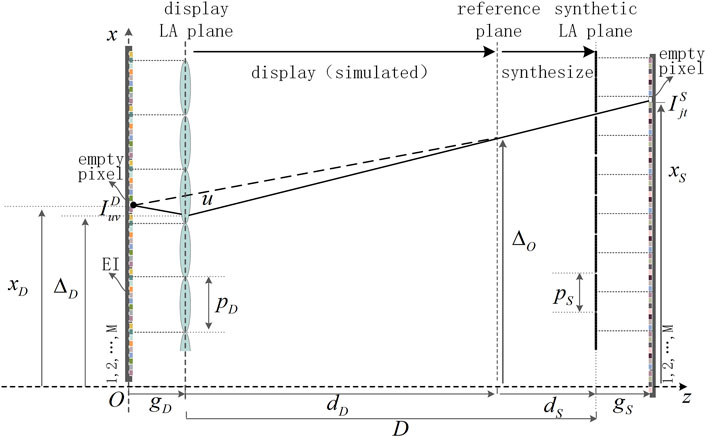
FIGURE 2. Principle of the SPOC algorithm.

Also, we can get the $x$ coordinate of the point where the ray intersects the display EIA plane, $x_D$, by using the intersection point with the reference plane and the optical center of the display lens $u$. Then, the index of the pixel where the ray intersects the display EIA plane, $v$, can be expressed as

$v=\frac{x_D-\left(u-1\right)\times p_D}{p_D/n_D}.(2)$

Here, $n_D$ is the number of pixels in each display EI, and the value of the display pixel, $I_{uv}^D$, is the value of the synthetic pixel, $I_{jt}^S$. Thus, the mapping relationship between the display pixels and the synthetic pixels is established, and a new EIA is obtained.

The SPOC algorithm uses only one simulated ray to establish the mapping relationship between the display pixels and the synthetic pixels, that is, the algorithm only considers the effect of the display lens that the ray intersects on the synthetic pixel. Thus, the contribution of other display lenses that can be covered by the rays passing through the upper and lower edges of the corresponding synthetic lens to the synthetic pixel has not been reflected. When real cameras are used to obtain perspective views, due to mechanical errors or operating errors, the display pixels in some EIs may have large errors or are even empty pixels and the synthetic pixels we get also have large errors or are even empty pixels.

We take photos of the virtual scene as the display EIA of the algorithm by using the software 3ds MAX. The structure of the capture system is shown in Figure 3A. The size of the virtual camera array we set is 23 × 23, and the overall arrangement is square. The distance between adjacent cameras is 2 mm, the FOV of the camera is 14.2°, and the pixel resolution of the image taken by the camera is 179 × 179. The virtual scene we set is composed of two cubic blocks, and the side length of the block is 20 mm. The surface of the building block is a pattern composed of white dots or the number “5,” and the front view of the virtual scene is shown in Figure 3B. The center of the left block is 60 mm away from the plane of the virtual camera array, and the center of the right block is 100 mm away from the plane of the virtual camera array. In the process of synthesizing the new EIA, we set the distance between the display LA plane and the synthetic LA plane to be 160 mm. When using the SPOC algorithm, the reference plane is set at the center of the two blocks, that is, at a distance of 80 mm away from the camera array. We use the rays passing through the upper edge, center, and lower edge of each synthetic lens in the synthetic LA to match the display pixels and the synthetic pixels, and the results are shown in Figure 4. This shows that when using the SPOC algorithm, if the position where the ray passes through each synthetic lens in the synthetic LA is different, then the display lens that the ray intersects will be different. Correspondingly, the value of the display pixel is also different, and the SEIA generated is also different.

FIGURE 3

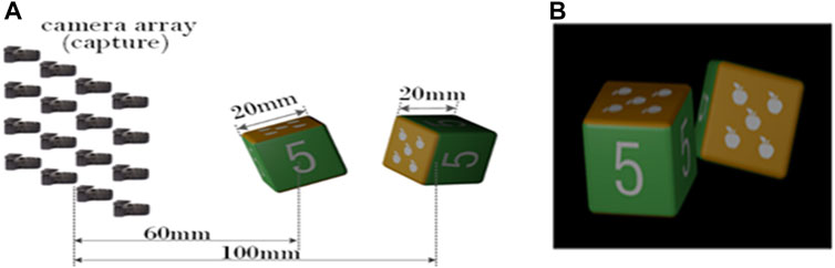
FIGURE 3. (A) Capture setting of the virtual scene. (B) Front view of the virtual scene.

FIGURE 4

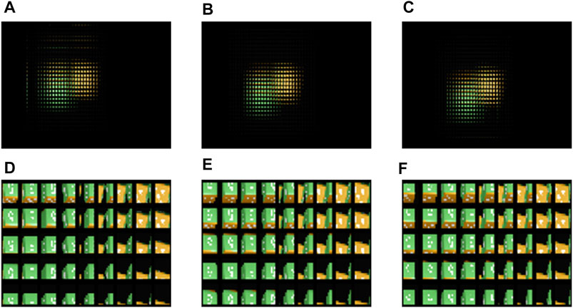
FIGURE 4. Effect of the SPOC algorithm: the first row from left to right is the overall display effect corresponding to the ray passing through the (A) upper edge, (B) center, and (C) lower edge of each synthetic lens. (D)–(F) are the corresponding central magnification renderings.

Principles of the Smart Pseudoscopic-to-Orthoscopic Conversion 1 Algorithm and the Average Smart Pseudoscopic-to-Orthoscopic Conversion Algorithm

Based on the above, we propose the SPOC1 algorithm, assuming that the synthetic pixel is converged by the rays passing through its corresponding synthetic lens. Three cases are considered, that is, the rays pass through the upper edge, center, and lower edge of the corresponding synthetic lens, respectively; then, we can get the display pixels corresponding to the three rays, and the average value of the display pixels is taken as the value of the synthetic pixel, thereby obtaining the mapping relationship between the synthetic pixels and the display pixels. Of course, for a certain synthetic pixel, the FOV of the display lenses corresponding to the rays passing through the upper and lower edges of the synthetic lens must be able to cover the synthetic lens.

The principle of the SPOC1 algorithm is shown in Figure 5. In a two-dimensional situation, the line, which passes through the display EIA plane and is perpendicular to the optical axis of the display LA, is taken as the $x$ axis, and the line, which passes through the optical axis of the bottom lens of the synthetic LA, is taken as the $z$ axis. To facilitate calculations, move the display device so that the bottom of the display LA is also on the $z$ axis and the intersection of the $z$ axis and the display EIA plane is the origin $o$. Thus, the coordinate system is established.

FIGURE 5

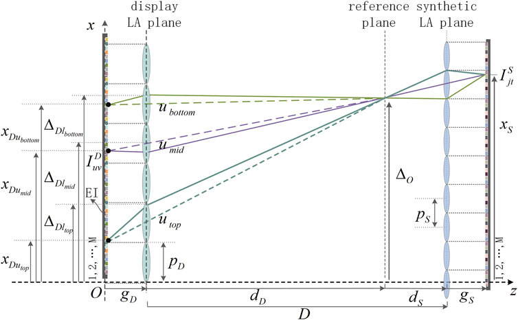
FIGURE 5. Principle of the SPOC1 algorithm.

The $z$ coordinate of the center of each SEI is equal to the $z$ coordinate of the center of the corresponding synthetic lens. The $x$ coordinate of the center of the $t^{th}$ pixel of the $j^{th}$ SEI (counting from 1), $x_S$, can be written as

$x_S=\left(j-1.5\right)p_S+t\frac{p_S}{n_S}.(3)$

Here, $n_S$ is the number of pixels in each SEI. The display LA and the synthetic LA are arranged compactly and have no gaps. The reference plane is located between the display LA plane and the synthetic LA plane. The ray $l$ passes through the center of the synthetic pixel and the optical center of the corresponding synthetic lens and intersects the reference plane. The $x$ coordinate of the intersection point, ${\Delta }_O$, can be expressed as

$\begin{array}{l}{\Delta }_0=\left(1+\frac{d_S}{g_S}\right)\left(j-1\right)p_S-\frac{d_S}{g_S}{x}_S.\\ \end{array}(4)$

The rays, $l_{top}$, $l_{mid}$, and $l_{bottom}$, pass through the upper edge, center, and lower edge of the corresponding synthetic lens, respectively, and the $x$ coordinates of the points where the rays intersect the display LA plane, ${\Delta }_{Dltop}$, ${\Delta }_{Dlmid}$, and ${\Delta }_{Dlbottom}$, can be calculated as

${\Delta }_{Dltop}=\left(j-0.5\right)p_S-\frac{D}{d_S}\left(\left(j-0.5\right)p_S-{\Delta }_O\right),(5)$

${\Delta }_{Dlmid}=\left(j-1\right)p_S-\frac{D}{d_S}\left(\left(j-1\right)p_S-{\Delta }_O\right),(6)$

${\Delta }_{Dlbottom}=\left(j-1.5\right)p_S-\frac{D}{d_S}\left(\left(j-1.5\right)p_S-{\Delta }_O\right).(7)$

The indexes of the display lenses corresponding to the rays, $l_{top}$, $l_{mid}$, and $l_{bottom}$, are $u_{top}$, $u_{mid}$, and $u_{bottom}$, respectively; then, we have

$u_{top}=Round\left(\frac{{\Delta }_{Dltop}}{p_D}\right),(8)$

$u_{mid}=Round\left(\frac{{\Delta }_{Dlmid}}{p_D}\right),(9)$

$u_{bottom}=Round\left(\frac{{\Delta }_{Dlbottom}}{p_D}\right).(10)$

Here, $p_D$ is the pitch of the display lens, and also the length of each display EI. The rays, $l_{top}$, $l_{mid}$, and $l_{bottom}$, pass through the optical center of the display lenses, $u_{top}$, $u_{mid}$, and $u_{bottom}$, respectively, and the $x$ coordinates of the points where the rays intersect the display EIA plane, $x_{Du}\left(u=u_{top},u_{mid},u_{bottom}\right)$, can be written as

$x_{Du}={\Delta }_O-\left(1+\frac{g_D}{D-d_S}\right)\left({\Delta }_O-p_D\left(u+0.5\right)\right),u=u_{top},u_{mid},u_{bottom}.(11)$

The indexes of the pixels where the rays, $l_{top}$, $l_{mid}$, and $l_{bottom}$, intersect the display EIA plane, $v_{jtu}\left(u=u_{top},u_{mid},u_{bottom}\right)$, can be expressed as

$v_{jtu}=Round\left(\left(x_{Du}-p_{D}u\right)\frac{n_D}{p_D}\right),u=u_{top},u_{mid},u_{bottom}.(12)$

The values corresponding to the display pixels where the rays, $l_{top}$, $l_{mid}$, and $l_{bottom}$, intersect the display EIA plane are $I_{uv}^D\left(u=u_{top},u_{mid},u_{bottom}\right)$. Therefore, the value of the synthetic pixel, $I_{jt}^S$, is the average value of $I_{uv}^D\left(u=u_{top},u_{mid},u_{bottom}\right)$, that is,

$I_{jt}^S=\frac{1}{3}{\displaystyle \sum I_{uv}^D},u=u_{top},u_{mid},u_{bottom}.(13)$

The block model is still used. When synthesizing the new EIA, $g_D$, $g_S$, $D$, and $d_D$ are 8, 8, 125, and 100 mm, respectively. The experiment is carried out according to the above method, and the result is shown in Figure 6. The SEIs generated by the SPOC algorithm have information loss and mosaic phenomenon, the relative position of the white dots in the pattern is distorted, the thickness of the digital “5” line is uneven, and the reconstruction effect is poor. The above problems also exist in the SEIs generated by the SPOC1 algorithm, but the information loss and the mosaic phenomenon have been alleviated. Thus, the SPOC1 algorithm is generally better than the SPOC algorithm. In addition, since the value of the synthetic pixel, $I_{jt}^S$, is the average value of $I_{uv}^D\left(u=u_{top},u_{mid},u_{bottom}\right)$, the pixel generated by the SPOC1 algorithm contains more information than that generated by the SPOC algorithm, which means that the SEI generated by the SPOC1 algorithm shows information that does not appear in the SEI generated by the SPOC algorithm at the same position and an increase in the number of rows and columns on the overall SEIA.

FIGURE 6

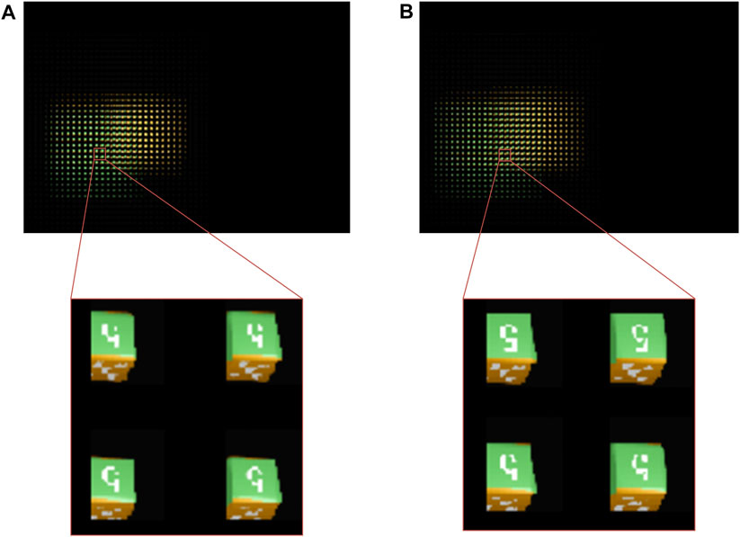
FIGURE 6. Overall and partial magnification effects: (A) SPOC algorithm and (B) SPOC1 algorithm.

However, we find that the quality of the SEIA generated by the SPOC1 algorithm is still not ideal. As we analyze further, the number of lenses between the display lenses $u_{top}$ and $u_{bottom}$, $N$, can be expressed as

$N=\frac{p_S\times d_D}{p_D\times d_S}.(14)$

The display lenses corresponding to the rays passing through the upper and lower edges of the synthetic lens may differ greatly (related to the selection of the reference plane, the pitch of the display lens, and the pitch of the synthetic lens). When $N\ge 3$, the contribution of the middle display lenses to the synthetic pixels is not well reflected. We revise the SPOC1 algorithm and propose the SPOC2 algorithm, that is, the average SPOC algorithm. These intermediate display lenses are taken into consideration, and the average value of the display pixels corresponding to the lenses between the display lenses $u_{top}$ and $u_{bottom}$ is taken as the value of the synthetic pixel.

Based on the principle of the SPOC1 algorithm shown in Figure 5, we demonstrate the principle of the average SPOC algorithm as shown in Figure 7. The rays pass through the optical centers of the lenses between the display lenses $u_{top}$ and $u_{bottom}$ (note $u_{top}\le u_{bottom}$), and the $x$ coordinates of the points where the rays intersect the display EIA plane, $x_{Du}\left(u_{top}\le u\le u_{bottom}\right)$, can be calculated as

$x_{Du}={\Delta }_O-\left(1+\frac{g_D}{D-d_S}\right)\left({\Delta }_O-p_D\left(u+0.5\right)\right),u_{top}\le u\le u_{bottom}.(15)$

FIGURE 7

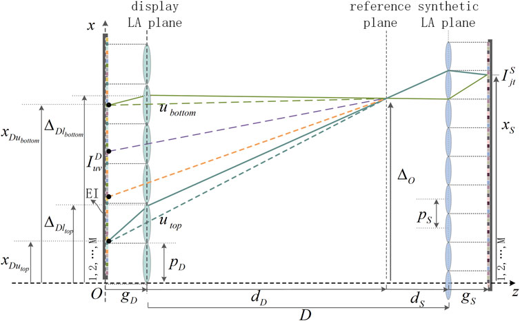
FIGURE 7. Principle of the average SPOC algorithm.

The indexes of the pixels where the rays intersect the display EIA plane, $v_{jtu}\left(u_{top}\le u\le u_{bottom}\right)$, can be expressed as

$v_{jtu}=Round\left(\left(x_{Du}-p_{D}u\right)\frac{n_D}{p_D}\right),u_{top}\le u\le u_{bottom}.(16)$

The values corresponding to the display pixels where the rays pass through the lenses between the display lenses $u_{top}$ and $u_{bottom}$ are $I_{uv}^D\left(u_{top}\le u\le u_{bottom}\right)$. The value of the synthetic pixel, $I_{jt}^S$, is the average value of $I_{uv}^D\left(u_{top}\le u\le u_{bottom}\right)$, that is,

$I_{jt}^S={\displaystyle \sum _{u=u_{top}}^{u=u_{bottom}}\frac{I_{uv}^D}{u_{bottom}-u_{top}+1}}.(17)$

Experimental Verification and Discussion

The conditions remain unchanged. The effect of the average SPOC algorithm is shown in Figure 8. The overall structure of the SEIA generated by the average SPOC algorithm is similar to that of the SEIA generated by the SPOC algorithm, but there are big differences in the partial SEIs. It is found that the quality of the SEIs has been improved when the average SPOC algorithm is applied, and there is almost no information loss or mosaic phenomenon. The relative position of the white dots in the pattern is correct and the line thickness of the number “5” is relatively uniform, which are similar to those of the block model. This shows that the reconstruction effect of the average SPOC algorithm is better. The SEIA generated by the average SPOC algorithm is displayed, and the display device is shown in Figure 9. It is composed of an LCD screen, LA, and displacement platform. Load the SEIA synthesized by the SPOC algorithm and the SEIA synthesized by the average SPOC algorithm on the screen of the SONY XPERIA mobile phone, with a resolution of 3,840 × 2,160 and each pixel size of 0.0315 mm, and the LA is arranged in a square with 50 rows and 50 columns. The unit lens specification is 2 mm × 2 mm, and the focal length is 8.2 mm. The displacement platform has high accuracy and can reach the requirement of a step of 0.01 mm.

FIGURE 8

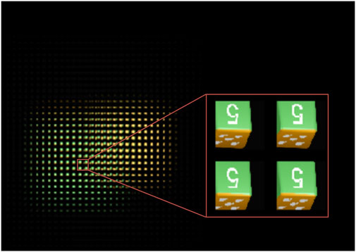
FIGURE 8. Overall and partial magnification effects of the average SPOC algorithm.

FIGURE 9

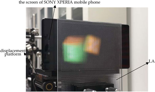
FIGURE 9. Experimental setup of the display system.

The three-dimensional reproduction results of the SPOC algorithm and the average SPOC algorithm are shown in Figure 10. The SPOC algorithm has poor reproduction effect, serious information loss, blurred number “5” and pattern composed of white dots, and mosaic phenomenon. However, the reproduction effect of the average SPOC algorithm is better, the information retention is good, the number “5” and the pattern composed of the white dots are clear and recognizable, and there is almost no mosaic phenomenon. In addition, in the left and right views, the patterns on the top and right side of the left block are almost indistinguishable in the SPOC algorithm, which is caused by pixel-matching errors. However, the patterns on the top and right side of the left block can be distinguished in the average SPOC algorithm and are more similar to the capture scene, indicating that, under the same conditions, the average SPOC algorithm alleviates the pixel-matching errors existing in the SPOC algorithm. Also, we find that the yellow and green areas on the block have little difference between the two algorithms, while the number “5” and the white dots are quite different. This indicates that the more complex the three-dimensional scene, the more obvious the advantage of the average SPOC algorithm.

FIGURE 10

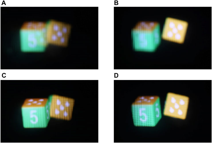
FIGURE 10. Three-dimensional reconstruction results. SPOC algorithm: (A) left 7.1° viewing angle and (B) right 7.1° viewing angle. Average SPOC algorithm: (C) left 7.1° viewing angle and (D) right 7.1° viewing angle.

The peak signal-to-noise ratio (PSNR) and structural similarity (SSIM) are used to evaluate the image quality. The images collected at a density of 23 × 23 are stitched into an EIA as a reference, and the SEIA generated by the SPOC algorithm and the SEIA generated by the average SPOC algorithm are compared under the above conditions. The results are shown in Table 1. It can be seen from Table 1 that, under the same conditions, the PSNR and SSIM values of the SEIA generated by the average SPOC algorithm are higher, which verifies the superiority of the average SPOC algorithm.

TABLE 1

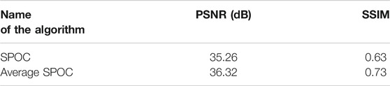
TABLE 1. Comparison of PSNR and SSIM values of the two algorithms.

Furthermore, we compare the two algorithms in the real three-dimensional scene. The scene is shown in Figure 11A, which consists of a tennis tube and a schoolbag. The tennis tube is located on the front side of the schoolbag, and the background of the scene is a green curtain. The camera array is a line array composed of 31 cameras, as shown in Figure 11B, and the focal length of the camera is 8 mm. The distance between adjacent cameras is 40 mm, which can realize the overall movement in the horizontal and vertical directions. In the acquisition process, after the camera array takes a set of pictures on the same line, it moves 20 mm to the left in the horizontal direction to take pictures again, thus completing the acquisition of one line of images. Then, the camera array moves 20 mm to the right to return to the shooting position of the previous set of pictures and moves up 20 mm in the vertical direction to start shooting another line of pictures. The above process is repeated 40 times, and we can obtain a 41 × 62 image array in which the resolution of each image is 1,981 × 1,981, which realizes the shooting effect of the 41 × 62 camera array, and the distance between adjacent rows and columns of the camera array is all 20 mm.

FIGURE 11

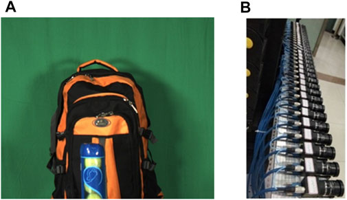
FIGURE 11. (A) Real three-dimensional scene. (B) Camera array.

In order to enable the display area to present the main body of the spatial scene, the parameters of the capture system need to be scaled, the equivalent distance between adjacent cameras is 2 mm, and the equivalent distance between the spatial scene and the camera array is 150 mm. When we synthesize the SEIA, the distance between the synthetic LA and the display LA is set to 235 mm, and the result is shown in Figure 12. The overall content of the SEIAs generated by the two algorithms is similar. However, comparing the part of the SEIAs, it is found that the SEIA generated by the SPOC algorithm is blurred. There are spots on the image, and the pixels at the spots have large errors or are even empty pixels. In the partial magnification effect shown in Figure 12A, the pattern on the tennis tube cannot be recognized. However, the details of the SEIA generated by the average SPOC algorithm are clearer. There are no spots on the image, and the content consistency is better. In the partial magnification effect shown in Figure 12B, the pattern on the tennis tube is clearly identifiable.

FIGURE 12

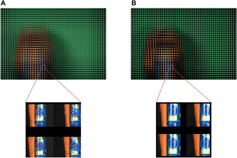
FIGURE 12. Overall and partial magnification effects: (A) SPOC algorithm and (B) average SPOC algorithm.

The three-dimensional reproduction results of the two algorithms are shown in Figure 13. Limited by the display system, the left and right viewing angles are small, but it can be recognized from the relative position of the tennis tube and the pattern in the middle of the schoolbag. It can be seen that the reproduction effect of the SPOC algorithm is poor, the information of the white zipper is almost completely lost, and the pattern in the middle of the schoolbag and the pattern on the tennis tube are blurred. However, the reproduction effect of the average SPOC algorithm is better, the information of the white zipper is well preserved, and the pattern in the middle of the schoolbag and the pattern on the tennis tube are clearly identifiable. The reproduction effect of the average SPOC algorithm is more similar to the capture scene. Also, we found that the yellow and black areas on the schoolbag have little difference between the two algorithms, while there is a big difference between the white zipper, the pattern on the schoolbag, and the pattern on the tennis tube, which also verifies that the more complex the spatial scene, the more obvious the advantage of the average SPOC algorithm.

FIGURE 13

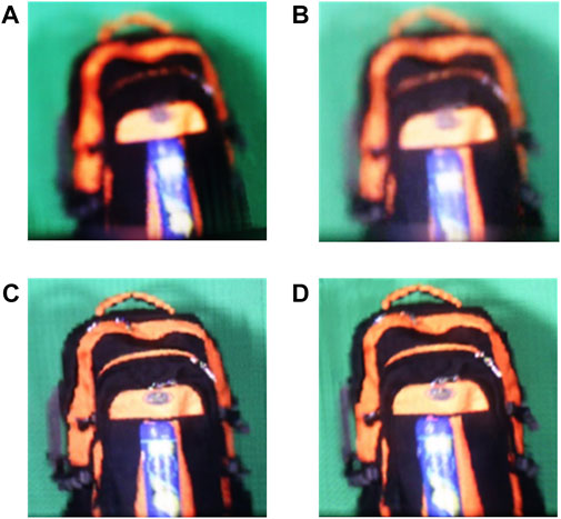
FIGURE 13. Three-dimensional reconstruction results. SPOC algorithm: (A) left 7.1° viewing angle and (B) right 7.1° viewing angle. Average SPOC algorithm: (C) left 7.1° viewing angle and (D) right 7.1° viewing angle.

Therefore, we believe that the middle lenses of the display lenses $u_{top}$ and $u_{bottom}$, where the rays passing through the upper and lower edges of the synthetic lens interact, respectively, also contribute to the synthetic pixel. When there are errors in the display pixel corresponding to the ray passing through the center of the synthetic lens, the pixels corresponding to these intermediate display lenses can be used to correct the errors, thereby improving the accuracy of the SEIA and the reconstruction effect. In particular, when $d_D$ is much larger than $d_S$, and $p_S$ is much larger than $p_D$, the improvement effect is more obvious.

Conclusion

The SPOC algorithm can synthesize a new SEIA by using the already captured EIA, but it also has disadvantages. We propose the average SPOC algorithm, which makes the converging effect of the synthetic lens on the ray reflected, and the display lenses that can converge at the synthetic pixel are considered. According to the principle of reversibility of the ray path, the rays start from the synthetic pixel and pass through the upper and lower edges of the corresponding synthetic lens. The average value of the display pixels corresponding to the display lenses that are covered by the rays is the value of the synthetic pixel, which reduces the matching errors between the synthetic pixels and the display pixels, mechanical errors, and operating errors in the SPOC algorithm. In addition, the average SPOC algorithm contains the information of the pixels corresponding to the display lenses that can be covered by the synthetic pixel, which means that more information can be obtained. Finally, we use the SEIAs generated by the SPOC algorithm and the average SPOC algorithm to actually restore the light field information of the three-dimensional scene, and the experimental results prove our theoretical analysis.

Data Availability Statement

The original contributions presented in the study are included in the article/supplementary material, and further inquiries can be directed to the corresponding authors.

Author Contributions

YM and XY conceptualized the idea. YM, WW, and XY performed the methodology. YM and ZY ran the software. YM, XJ, and CW validated the data. YM performed formal analysis, curated the data, wrote the original draft, and reviewed and edited the paper. ZY obtained the resources. XJ visualized the data. WW supervised the work. XY administered the project and acquired the funding. All authors have read and agreed to the published version of the manuscript.

Funding

This research was funded by the National Key Research and Development Program of China (2017YFB1104500) and National Natural Science Foundation of China (61775240).

Conflict of Interest

The authors declare that the research was conducted in the absence of any commercial or financial relationships that could be construed as a potential conflict of interest.

References

1. Okoshi T. Three-Dimensional Displays. Proc IEEE (1980) 68(5):548–64. doi:10.1109/proc.1980.11695

CrossRef Full Text | Google Scholar

2. Lippmann G. Épreuves réversibles donnant la sensation du relief. J Phys Theor Appl (1908) 7(1):821–5. doi:10.1051/jphystap:019080070082100

CrossRef Full Text | Google Scholar

3. Martínez-Corral M, Javidi B. Fundamentals of 3D Imaging and Displays: A Tutorial on Integral Imaging, Light-Field, and Plenoptic Systems. Adv Opt Photon (2018) 10(3):512–66. doi:10.1364/aop.10.000512

CrossRef Full Text | Google Scholar

4. Ives HE. Optical Properties of a Lippmann Lenticulated Sheet. J Opt Soc Am (1931) 21(3):171–6. doi:10.1364/josa.21.000171

CrossRef Full Text | Google Scholar

5. Chutjian A, Collier RJ. Recording and Reconstructing Three-Dimensional Images of Computer-Generated Subjects by Lippmann Integral Photography. Appl Opt (1968) 7(1):99–103. doi:10.1364/ao.7.000099

PubMed Abstract | CrossRef Full Text | Google Scholar

6. Okano F, Hoshino H, Arai J, Yuyama I. Real-time Pickup Method for a Three-Dimensional Image Based on Integral Photography. Appl Opt (1997) 36(7):1598–603. doi:10.1364/ao.36.001598

PubMed Abstract | CrossRef Full Text | Google Scholar

7. Erdmann L, Gabriel KJ. High-Resolution Digital Integral Photography by Use of a Scanning Microlens Array. Appl Opt (2001) 40(31):5592–9. doi:10.1364/ao.40.005592

PubMed Abstract | CrossRef Full Text | Google Scholar

8. Jang J-S, Javidi B. Formation of Orthoscopic Three-Dimensional Real Images in Direct Pickup One-Step Integral Imaging. Opt Eng (2003) 42(7):1869–70. doi:10.1117/1.1584054

CrossRef Full Text | Google Scholar

9. Martínez-Corral M, Javidi B, Martínez-Cuenca R, Saavedra G. Formation of Real, Orthoscopic Integral Images by Smart Pixel Mapping. Opt Express (2005) 13(23):9175–80. doi:10.1364/opex.13.009175

PubMed Abstract | CrossRef Full Text | Google Scholar

10. Park KS, Min S-W, Cho Y. Viewpoint Vector Rendering for Efficient Elemental Image Generation. IEICE Trans Inf Syst (2007) E90-D(1):233–41. doi:10.1093/ietisy/e90-1.1.233

CrossRef Full Text | Google Scholar

11. Min S-W, Park KS, Lee B, Cho Y, Hahn M. Enhanced Image Mapping Algorithm for Computer-Generated Integral Imaging System. Jpn J Appl Phys (2006) 45(7L):L744–L747. doi:10.1143/jjap.45.l744

CrossRef Full Text | Google Scholar

12. Shin D-H, Tan C-W, Lee B-G, Lee J-J, Kim E-S. Resolution-Enhanced Three-Dimensional Image Reconstruction by Use of Smart Pixel Mapping in Computational Integral Imaging. Appl Opt (2008) 47(35):6656–65. doi:10.1364/ao.47.006656

PubMed Abstract | CrossRef Full Text | Google Scholar

13. Zhang J, Wang X, Chen Y, Zhang Q, Yu S, Yuan Y, et al. Feasibility Study for Pseudoscopic Problem in Integral Imaging Using Negative Refractive index Materials. Opt Express (2014) 22(17):20757. doi:10.1364/oe.22.020757

PubMed Abstract | CrossRef Full Text | Google Scholar

14. Yu X, Sang X, Gao X, Chen Z, Chen D, Duan W, et al. Large Viewing Angle Three-Dimensional Display With Smooth Motion Parallax and Accurate Depth Cues. Opt Express (2015) 23(20):25950. doi:10.1364/oe.23.025950

PubMed Abstract | CrossRef Full Text | Google Scholar

15. Chen J, Wang QH, Li SL, Xiong ZL, Deng H. Multiple Elemental Image Mapping for Resolution‐Enhanced Orthographic View Image Generation Based on Integral Imaging. J Soc Inf Disp (2015) 22(7–9):487–92. doi:10.1002/jsid.273

CrossRef Full Text | Google Scholar

16. Wang Z, Lv G, Feng Q, Wang A. A Fast-Direct Pixel Mapping Algorithm for Displaying Orthoscopic 3D Images With Full Control of Display Parameters. Opt Commun (2018) 427:528–34. doi:10.1016/j.optcom.2018.06.067

CrossRef Full Text | Google Scholar

17. Zhang H-L, Deng H, Ren H, Yang X, Xing Y, Li D-H, et al. Method to Eliminate Pseudoscopic Issue in an Integral Imaging 3D Display by Using a Transmissive Mirror Device and Light Filter. Opt Lett (2020) 45(2):351. doi:10.1364/ol.45.000351

CrossRef Full Text | Google Scholar

18. Navarro H, Martínez-Cuenca R, Saavedra G, Martínez-Corral M, Javidi B. 3D Integral Imaging Display by Smart Pseudoscopic-To-Orthoscopic Conversion (SPOC). Opt Express (2010) 18(25):25573–83. doi:10.1364/oe.18.025573

PubMed Abstract | CrossRef Full Text | Google Scholar

19. Shen X, Martinez Corral M, Javidi B. Head Tracking Three-Dimensional Integral Imaging Display Using Smart Pseudoscopic-To-Orthoscopic Conversion. J Disp Technol (2016) 12(6):542–8. doi:10.1109/jdt.2015.2506615

CrossRef Full Text | Google Scholar

20. Martínez-Corral M, Dorado A, Navarro H, Saavedra G, Javidi B. Three-Dimensional Display by Smart Pseudoscopic-to-Orthoscopic Conversion With Tunable Focus. Appl Opt (2014) 53(22):E19–E25. doi:10.1364/ao.53.000e19

PubMed Abstract | CrossRef Full Text | Google Scholar

21. Xiao X, Shen X, Martinez-Corral M, Javidi B. Multiple-Planes Pseudoscopic-to-Orthoscopic Conversion for 3D Integral Imaging Display. J Disp Technol (2015) 11(11):921–6. doi:10.1109/jdt.2014.2387854

CrossRef Full Text | Google Scholar

22. Yan Z, Jiang X, Yan X. Performance-Improved Smart Pseudoscopic to Orthoscopic Conversion for Integral Imaging by Use of Lens Array Shifting Technique. Opt Commun (2018) 420:157–62. doi:10.1016/j.optcom.2018.03.061

CrossRef Full Text | Google Scholar

23. Yang S, Sang X, Yu X, Gao X, Yang L, Liu B, et al. High Quality Integral Imaging Display Based on Off-Axis Pickup and High Efficient Pseudoscopic-to-Orthoscopic Conversion Method. Opt Commun (2018) 428:182–90. doi:10.1016/j.optcom.2018.07.021

CrossRef Full Text | Google Scholar

24. Huang Y, Yan Z, Jiang X, Jing T, Chen S, Lin M, et al. Performance Enhanced Elemental Array Generation for Integral Image Display Using Pixel Fusion. Front Phys (2021) 9:97. doi:10.3389/fphy.2021.639117

CrossRef Full Text | Google Scholar