Numerical Study of Divergence Cleaning and Coronal Heating/Acceleration Methods in the 3D COIN-TVD MHD Model

Introduction

The 3D COIN-TVD MHD model which was proposed in [1–3] and was improved in [4–8] in recent years can effectively realize the coronal–interplanetary 3D solar wind simulation. This model uses the TVD Lax–Friedrichs (TVD-LF) scheme uniformly in the corona region and the interplanetary space region, and a combination of Open Multi-Processing (OpenMP) based on shared memory and Message Passing Interface (MPI) based on distributed memory has been successfully used to study the solar wind background from the corona to the interplanetary space.

The solar energy is stored in the solar nucleus, and the generated radiant energy spreads from the inside to the outside. The solar temperature should theoretically decrease with the increase of the heliocentric distance. However, the temperature of the upper atmosphere corona is much higher than that of the lower atmosphere (photosphere). The reason for the abnormal warming of the atmosphere has not yet been investigated. Therefore, coronal heating/acceleration is a central issue in the solar coronal simulation and has been discussed by many researchers (e.g., [9–16]). Parker proposed a basic theory for the problem of heating an expanding solar corona [17–19]. Later, various methods for solar wind acceleration and coronal heating have been developed. For example, the Alfvén wave heating method (AHM) can accelerate solar wind through the exchange of momentum and energy between large-scale Alfvén wave turbulence and solar wind plasma [10]. The turbulent heating method (THM) assumes that the turbulent free energy is transformed into the energy accelerated by the solar wind when the turbulent free energy changes with the heliocentric distance [10]; By adding momentum and energy source terms to the MHD equations [16], the volume heating method (VHM) has been widely used in solar wind simulation (e.g., [15, 20, 21].

In the MHD simulation, the divergence of the magnetic field should be strictly controlled to zero. The nonzero divergence of the magnetic field can lead to the $\nabla \cdot \mathit{B}$ error during the calculation. When this occurs, numerical instability may develop and the simulation can break down. Therefore, scientists have proposed many methods to control the divergence of the magnetic field, such as the generalized Lagrange multiplier (GLM) method [22–24], the CT method [21, 25–27], the projection method [28], the vector potential method [29, 30], the Powell method [31, 32], the diffusion method [7] and the globally solenoidality-preserving (GSP) method [33].

In this study, we adopt the COIN-TVD model to simulate the coronal solar wind. Similar to [20, 21], we use the volume heating sources to model the solar wind heating/acceleration process in the simulation.

In Governing Equations of Coronal Interplanetary-Total Variation Diminishing Model, we introduce the equations of the COIN-TVD MHD model. Mesh Grid System and Numerical Scheme describes mesh grid system and boundary conditions. Volume Heating Method and Magnetic Field Divergence Cleaning Methods presents the VHM method and three magnetic field divergence processing methods. Numerical Results shows the results of numerical simulation and comparisons of three methods for processing magnetic field divergence. In Conclusions and Discussions, we make the conclusion and discussion.

Governing Equations of Coronal–Interplanetary Total Variation Diminishing Model

The ideal MHD equations are used to simulate the coronal solar wind. Under the Corotating coordinate system, equations can be written as:

$\frac{\partial \rho }{\partial t}+\nabla \cdot \left(\rho \mathit{v}\right)=0(1)$

$\left(\frac{\partial \rho \mathit{v}}{\partial t}\right)+\nabla \cdot \left[\left(\mathit{P}+\frac{{\mathit{B}}^2}{2{\mu }_0}\right)\mathit{I}+\rho \mathit{v}\mathit{v}-\frac{\mathit{B}\mathit{B}}{{\mu }_0}\right]=-\frac{\rho G{M}_s}{r^2}\frac{\mathit{r}}{r}+\rho \mathit{f}(2)$

$\frac{\partial \mathit{B}}{\partial t}+\nabla \cdot \left(\mathit{v}\mathit{B}-\mathit{B}\mathit{v}\right)=0(3)$

$\frac{\partial \mathit{P}}{\partial t}+\nabla \cdot \left(\mathit{\rho }\mathit{v}\right)=-\left(\gamma -1\right)\mathit{P}\nabla \cdot \mathit{v}(4)$

where $\rho$ is the mass density, $\mathit{v}$ is the plasma velocity, B is the magnetic field, P is pressure, ${\mu }_0$ is the magnetic permeability of free space, I is the unit tensor, G is the gravitational constant, $M_s$ is the solar mass, $\mathit{f}=-\mathit{\omega }\times \left(\mathit{\omega }\times \mathit{r}+2\mathit{\omega }\times \mathit{v}\right)$ is the additional fictitious force densities, in which $\mathit{\omega }$ is the angular velocity of the rotation, and $\gamma$ is the polytrophic index, which is set to be 1.05 in this study.

Mesh Grid System and Numerical Scheme

Mesh Grid System

In the spherical coordinate, the range of the calculation area is expressed as 1$\text{Rs}\le r\le 22.5\text{Rs},$$-\frac{\text{π}}{2}\le \theta \le \frac{\text{π}}{2},$ and $0\le \varnothing \le 2\text{π},$ where r is the radial distance from the solar center to the solar surface, $\theta$ is latitude, and $\varnothing$ is longitude. To avoid the singularity, the computation domain is divided into six identical component meshes to envelop a spherical surface with partial overlap on their boundaries [34]. The following grid partitions are employed; the grid mesh is built in the form of $224\left(r\right)\times 180\left(\theta \right)\times 360(\varnothing )$. The radial direction uses a proportional grid, the radial step length increases from 0.0161R_S at the inner boundary of 1R_S to 0.3636R_S at the outer boundary near 22.5R_S, and the total number of grids at r-direction is 224. In the latitudinal and longitudinal directions, the grid resolution is $\Delta \theta =\Delta \varnothing =1^{\circ }$.

Numerical Scheme

In the COIN-TVD model, all of the physical quantities are computed from the TVD-LF numerical scheme in a face-centered grid structure (e.g., [7, 8]). And this scheme is performed in the six-component mesh grid system.

The inner boundary is located on the surface of the Sun, where the inner boundary setting depends on local fluid conditions (e.g., [2]; 2007, [16, 21, 33]). When $v_r>0$, $\rho ={\rho }_0$, and $T=T_0$, $\mathit{B}={\mathit{B}}_0$, and $\nabla \cdot \left(\rho \mathit{v}\right)=0$; when $v_r<0$, $\partial \rho /\partial r=0$, $\partial T/\partial r=0$, $\mathit{B}={\mathit{B}}_0$, v = 0.

The Carrington Rotation (CR) 2199 is chosen for background establishment. The initial magnetic field B₀ is given by using the potential field source surface (PFSS) model [35, 36], the spherical harmonics coefficients were used to obtain the initial PFSS solution is 6. And other initial parameters, such as plasma density $\text{ρ}$₀, temperature T₀, and velocity v, are calculated by Parker’s solar wind flow solution [17]. The temperature and the number density on the solar surface are set to be 1.5 × 10⁶ K and 1.67 × 10⁸ cm⁻³, respectively. The boundary condition of the magnetic field at the inner surface also remains fixed all through the simulation. The parameters at the outer boundary are set according to the projected characteristic boundary conditions e.g., [32, 37, 38].

Volume Heating Method and Magnetic Field Divergence Cleaning Methods

In this section, we introduce the numerical schemes of the volume heating method and three methods to constrain $\nabla \cdot \mathit{B}$ in MHD simulation.

Volume Heating Method

Due to the limitations of observation and theory, there is no mature theoretical model to describe the mechanism of coronal heating and solar wind acceleration. Here, we use the volume heating method to solve the issue of coronal heating and solar wind acceleration. We add the source terms of momentum S_M and energy Q_E to the MHD Eq. 1, Eq. 2, Eq. 3, and Eq. 4 as follows:

$\frac{\partial \rho }{\partial t}+\nabla \cdot \left(\rho \mathit{v}\right)=0(5)$

$\left(\frac{\partial \rho \mathit{v}}{\partial t}\right)+\nabla \cdot \left[\left(\mathit{P}+\frac{{\mathit{B}}^2}{2{\mu }_0}\right)\mathit{I}+\rho \mathit{v}\mathit{v}-\frac{\mathit{B}\mathit{B}}{{\mu }_0}\right]=-\frac{\rho G{M}_s}{r^2}\frac{\mathit{r}}{r}+\rho \mathit{f}+S_M(6)$

$\frac{\partial \mathit{B}}{\partial t}+\nabla \cdot \left(\mathit{v}\mathit{B}-\mathit{B}\mathit{v}\right)=0(7)$

$\frac{\partial \mathit{P}}{\partial t}+\nabla \cdot \left(\rho \mathit{v}\right)=-\left(\gamma -1\right)\mathit{P}\nabla \cdot \mathit{v}+\left(\gamma -1\right)Q_E(8)$

According to the work in [7, 39–41], we set energy and momentum source terms as follows:

$\begin{array}{l}{Q}_E=Q_1\left(r-1\right)e^{\left(-r/L_{Q_1}\right)}\\ S_M=S_1\left(r-1\right)e^{\left(-r/L_M\right)}\end{array}(9)$

Here, $\text{γ}=1.05$, which is the polytrophic index. In the calculation region, the polytropic index γ need not be set very large. γ = 1.05 can heat the corona and accelerate solar wind.

Here, r is the heliocentric distance, $Q_1$ and $L_{Q_1}$ are the intensity and attenuation length of heating, and $S_1$ and $L_M$ are the intensity and decay length of the momentum addition. The parameters $L_{Q_1}$ and $L_M$ are set to be 1, $Q_1=Q_0{C}_a$, and $S_1=S_0{C}_a$. To test the influence of the parameter of energy and momentum source terms, we set two groups of different parameters for comparison. In model A, we set: $Q_0=6\times {10}^{-10}J\cdot m^{-3}\cdot s^{-1}$, $S_0=7.6\times {10}^{-14}N\cdot m^{-3}$ and $C_a=\frac{\left(1-0.8e^{{\left(-{\left({\theta }_b/1\right)}^2\right)}^2}\right)}{{\left(1+f_s\right)}^{9/2}}$ and find that the coronal heating and solar wind acceleration were not obvious. In model B, we adjust the parameters based on [33], which are $Q_0=6\times {10}^{-8}J\cdot m^{-3}\cdot s^{-1}$, $S_0=7.9\times {10}^{-14}N\cdot m^{-3}$ and $C_a=\frac{C_{a\prime }}{max{C}_{a\prime }}$, where $C_a^{\text{'}}=\frac{\left(1-0.8e^{{\left(-{\left({\theta }_b/1\right)}^1\right)}^1}\right)}{{\left(1+f_s\right)}^{9/2}}$. Here, $f_s={\left(\frac{R_s}{R_{ss}}\right)}^2\frac{{\mathit{B}}_{R_s}}{{\mathit{B}}_{R_{ss}}}$ is the expansion factor, where Rs is the solar radius, R_SS = 2.5R_S, and ${\mathit{B}}_{R_S}$ and ${\mathit{B}}_{R_{SS}}$ are magnetic field strength at the solar surface and at $R_{SS}$, respectively. Inspired by the Wang–Sheeley–Arge (WSA) model [42, 43], the solar wind speed is related to the magnetic field expansion factor $f_s$ and the minimum angular distance ${\theta }_b$. As $f_s$ increases, the speed decreases, the high-speed stream originating from the center of the open field region always has large ${\theta }_b$, and the low-speed stream from the coronal hole boundary has a relatively small ${\theta }_b$.

Following [20, 44, 45], the source term Q_E also contains a heat conduction term, the expression of the heat conduction term is $\nabla \left(\xi T^{\frac{5}{2}}\frac{\nabla T\cdot \mathit{B}}{{\mathit{B}}^2}\right)\cdot \mathit{B}$, $\text{ξ}$ is the collisional thermal conductivity parallel to the magnetic field as given in [46] and the proton and electron temperatures are equal to T. If we add the heat conduction term in the Q_E, the partial differential in the formula decreases the calculation accuracy. And after the research in [45], many works (e.g., Feng, 2012, [21]; 2017 [33]) verify that without adding heat conduction item, the coronal solar wind can also be accelerated and heated.

Powell Method

The Powell method to maintain the magnetic divergence cleaning constraint is given as follows.

Two divergence source terms, $-\left(\nabla \cdot \mathit{B}\right)\mathit{B}$ and $-\left(\nabla \cdot \mathit{B}\right)\mathit{v}$, are added separately on the right side of Eq. (6) and Eq. (7) to get the following MHD equations:

$\{\begin{array}{c}\frac{\partial \rho }{\partial t}+\nabla \cdot \left(\rho \mathit{v}\right)=0\\ \left(\frac{\partial \rho \mathit{v}}{\partial t}\right)+\nabla \cdot \left[\left(\mathit{P}+\frac{{\mathit{B}}^2}{2{\mu }_0}\right)\mathit{I}+\rho \mathit{v}\mathit{v}-\frac{\mathit{B}\mathit{B}}{{\mu }_0}\right]=-\frac{\rho G{M}_s}{r^2}\frac{\mathit{r}}{r}+\rho \mathit{f}+S_M-\left(\nabla \cdot \mathit{B}\right)\mathit{B}\\ \frac{\partial \mathit{B}}{\partial t}+\nabla \cdot \left(\mathit{v}\mathit{B}-\mathit{B}\mathit{v}\right)=-\left(\nabla \cdot \mathit{B}\right)\mathit{v}\\ \frac{\partial \mathit{P}}{\partial t}+\nabla \cdot \left(\rho \mathit{v}\right)=-\left(\gamma -1\right)\mathit{P}\nabla \cdot \mathit{v}+\left(\gamma -1\right)Q_E\end{array}(10)$

In this way, the divergence of the magnetic field can be propagated to the boundary to reduce the numerical error of $\nabla \cdot \mathit{B}$ in the computational region [31]. From Eq. 10 with the source term, the quantity $\nabla \cdot \mathit{B}/\rho$ satisfies the advection equation, which is,

$\frac{\partial }{\partial t}\left(\frac{\nabla \cdot \mathit{B}}{\rho }\right)+\nabla \cdot \left(\mathit{v}\cdot \frac{\nabla \cdot \mathit{B}}{\rho }\right)=0(11)$

This means that the $\nabla \cdot \mathit{B}$ must be transported by the plasma motions when Powell correction is applied, since the initial and boundary conditions satisfy $\nabla \cdot \mathit{B}=0$, and the $\nabla \cdot \mathit{B}$ will be near zero for all later times throughout the simulation.

Diffusive Method

The diffusive method is proposed to reduce the error of the magnetic divergence, in which an artificial diffusivity is added at each time step as $\frac{\partial \mathit{B}}{\partial t}=\eta \nabla \left(\nabla \cdot \mathit{B}\right)$. Under the condition of $\Delta t\le \mu \frac{{\left(\Delta x\right)}^2}{\eta }$, where $\mu \in \left(\mathrm{0,2}\right)$, the error of the magnetic divergence is diffused away at the maximal rate allowed by iterating:

${\mathit{B}}^{k+1}={\mathit{B}}^k+\mu {\left(\Delta x\right)}^2\nabla \nabla \cdot {\mathit{B}}^k,k=\mathrm{0,1,2......}K(12)$

Here, ${\left(\Delta x\right)}^2=\frac{1}{\frac{1}{{\left(\Delta r\right)}^2}+\frac{1}{{\left(r\Delta \theta \right)}^2}+\frac{1}{{\left(r\sin \theta \Delta \varnothing \right)}^2}}$

For satisfying the condition $\max \left(\frac{{\displaystyle \iint B_{n}ds}}{{\displaystyle \iint \left|B_n\right|ds}}\right)\le {10}^{-2}$, less than ten iterations are needed at each time step. This method does not violate shock capturing property, at least to the second-order accuracy in smooth regions [8, 47].

Composite Diffusive/Powell Method

We combined the Powell method and the diffusive method together in the MHD calculation in the composite diffusive/Powell method for the first time, and this method can further control the error of the magnetic field divergence.

The composite diffusive/Powell method adds two divergence source terms, $-\left(\nabla \cdot \mathit{B}\right)\mathit{B}$ and $-\left(\nabla \cdot \mathit{B}\right)\mathit{v}$, to Eq. 6 and Eq. 7 to get Eq. 10. The divergence of the magnetic field can be propagated to the boundary, and the quantity $\nabla \cdot \mathit{B}/\rho$ satisfies the advection equation (Eq. 11). When solving the equation, the error of magnetic divergence is diffused away at the maximal rate allowed by iterating Eq. 12.

Numerical Results

In this section, we show the numerical results of the solar coronal simulation from 1R_S to 22.5R_S for CR2199, which are obtained by executing the methods introduced in Volume Heating Method and Magnetic Field Divergence Cleaning Methods.

It takes about 100 h in physical time to obtain the steady state in our simulation. Figures 1,2 present the distribution of the magnetic field lines, the radial velocity, the number density and the temperature on the meridional plane at Φ = 180°–0° from model A and model B, respectively. From these figures, it can be seen that the high latitude areas always have fast speed, high temperature, and low density. On the contrary, the radial speed is slower, the temperature is lower, and the number density is higher at lower latitudes around the heliospheric current sheet (HCS), and this is the characteristic feature of the solar wind in the corona [47]. Model B is successful in simulating the acceleration and heating of the solar wind in the corona, as shown in Figure 2. Compared with Figure 1, we can find that both the radial speed and temperature in Figure 2 are higher than those in Figure 1 obviously. This result indicates that the VHM can accelerate and heat the coronal solar wind, and the parameters $S_0$, $Q_0$, and $C_a$ in VHM can affect the coronal heating and solar wind acceleration process significantly.

FIGURE 1

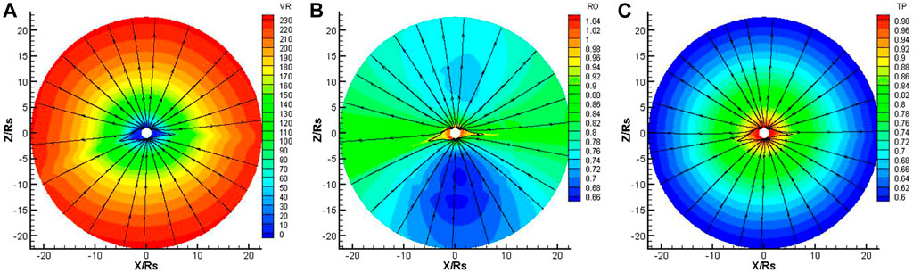
FIGURE 1. The distribution of the radial speed VR (km/s) (A), density RO × 10⁸ (/cm³) (B) and temperature TP × 10⁶ (K) (C) on the meridional plane of Φ = 180°–0° from 1 to 22.5R_s, deduced from model A. The streamline represents the magnetic field lines.

FIGURE 2

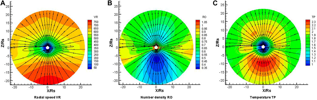
FIGURE 2. The distribution of the radial speed VR (km/s) (A), density RO × 10⁸ (/cm³) (B) and temperature TP × 10⁶ (K) (C) on the meridional plane of Φ = 180°–0° from 1 to 22.5R_s, deduced from model B. The streamline represents the magnetic field lines.

Then, we present the simulation results of the coronal solar wind with three magnetic divergence cleaning methods. Figures 3–5, respectively, show the variation in the radial speed, the number density, and the temperature along heliocentric distance from 1 to 22.5 Rs with different latitudes of θ = −80° and θ = −10° at the same longitude of Φ = 0°, where θ = −80° locates at the open field region and θ = −10° locates at the HCS region. Comparing the three figures, we can find that the radial speed in the open field region is larger than that in the HCS region, the temperature is higher in the open field, and the number density is smaller in the high latitude region.

FIGURE 3

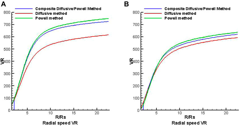
FIGURE 3. The distribution of radial speed VR (km/s) along heliocentric distance with different latitudes of θ = −80° (A) and θ = −10° (B) at the same longitude Φ = 0° from three divergence methods.

FIGURE 4

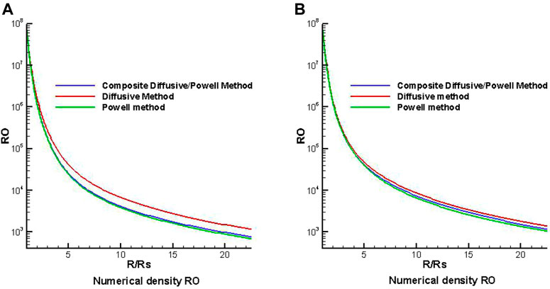
FIGURE 4. The distribution of density RO (/cm³) along heliocentric distance with different latitudes of θ = −80° (A) and θ = −10° (B) at the same longitude Φ = 0° from three divergence methods.

FIGURE 5

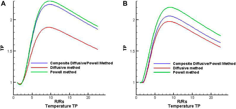
FIGURE 5. The distribution of temperature TP × 10⁶ (K) along heliocentric distance with different latitudes of θ = −80° (A) and θ = −10° (B) at the same longitude Φ = 0° from three divergence methods.

The composite diffusive/Powell method which combines the diffusive method and the Powell method is our new try to handle the $\nabla \cdot B$ constraint. From Figures 3–5, we can also see that the curve from the composite diffusive/Powell method is always in the middle, so it can generate a stable solar wind structure like the other two methods.

To quantitatively see how $\nabla \cdot \mathit{B}$ evolves, we define the relative divergence error [48] as follows:

$Error\left(\mathit{B}\right)=\frac{\left|\nabla \cdot \mathit{B}\right|\Delta h}{\left|\mathit{B}\right|}(13)$

Here, $\Delta h=\sqrt{\frac{3}{\frac{1}{{\left(\Delta r\right)}^2}+\frac{1}{{\left(r\Delta \theta \right)}^2}+\frac{1}{{\left(r\sin \theta \Delta \varnothing \right)}^2}}}$ is the characteristic length of the mesh element.

To investigate how the three magnetic divergence cleaning methods control the $\nabla \cdot \mathit{B}$ error quantitaitvely, we make a numerical comparison for the Error(B) among the three methods.

Figures 6,7 show the distributions of the Error(B) on the different meridional planes of Φ = 180°–0° and Φ = 270°–90°, respectively, for the steady-state solar wind. The three panels in Figures 6, 7 present the results from the composite diffusive/Powell method, the diffusive method and the Powell method, from left to right, respectively. It is obvious that the Error(B) deduced from the composite diffusive/Powell method is lower than that from the other two methods, on both meridional planes. This indicates that the composite diffusive/Powell method is the most effective method among the three methods in dealing with the magnetic field divergence.

FIGURE 6

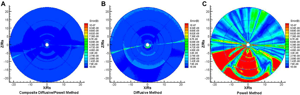
FIGURE 6. The distribution of Error(B) on the meridional plane of Φ = 180°–0° from 1 to 22.5R_S, from composite diffusive/Powell method (A), diffusive method (B), and Powell method (C), respectively.

FIGURE 7

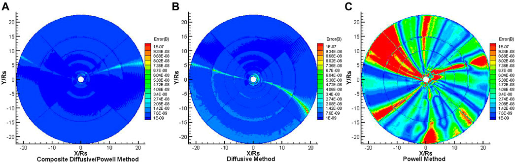
FIGURE 7. The distribution of Error(B) on the meridional plane of Φ = 270°–90° from 1 to 22.5R_S, the results from composite diffusive/Powell method (A), diffusive method (B) and Powell method (C), respectively.

Here, we use the following metric for measuring divergence, which was also adopted by other research studies (e.g., [33, 47]):

$Error{\left(\mathit{B}\right)}^{ave}={\displaystyle \sum }_{k=1}^M\frac{\left|\nabla \cdot \mathit{B}\right|\Delta h}{\left|\mathit{B}\right|}/M(14)$

where M is the total number of grid points in the computational domain. We know that there are other metrics that can be used to measure the divergence. As pointed in [49], the metric defined by Eq. 14 may rely on the spatial resolution. However, in this simulation, we make the comparison among the three cases with the same mesh system and the same metric definition; therefore, the influence of the spatial resolution on the comparison of the metric by Eq. 14 can be ignored.

Figure 8 shows the evolution of the Error(B)^ave with time deduced from the three methods. It can be recognized that the value of the Error(B)^ave from the composite diffusive/Powell method is around 10^–8.7–10^–8.5, from the diffusive method is around 10^–8.6–10^–8.2, and from the Powell method is around 10^–8.6–10^–7.1. The composite diffusive/Powell method has the smallest Error(B)^ave, and this method is a new try to maintain the magnetic divergence-free constraint. From Figure 8, we can also find that the Error(B)^ave from the composite diffusive/Powell method and diffusive method is smaller than that from the Powell method obviously. Moreover, the Error(B)^ave from the composite diffusive/Powell method keeps on decreasing after 60 h and is significantly smaller than that from the diffusive method near 100 h. Overall, we can find that all the divergence cleaning methods can keep the related errors under control, though the divergence errors of the Powell method are larger than those of the other methods, the divergence errors shown in Figures 6–8 are indeed small, and the largest worst number is 10^–7, shown as the orange and red colors in Figures 6,7. The Error(B)^ave from the Powell method is about 10^–7.3, from the diffusive method is 10^–8.4, and from the composite diffusive/Powell method is 10^–8.7 near 100 h. The composite diffusive/Powell method is the best method to reduce the error of magnetic divergence among the three methods in this research.

FIGURE 8

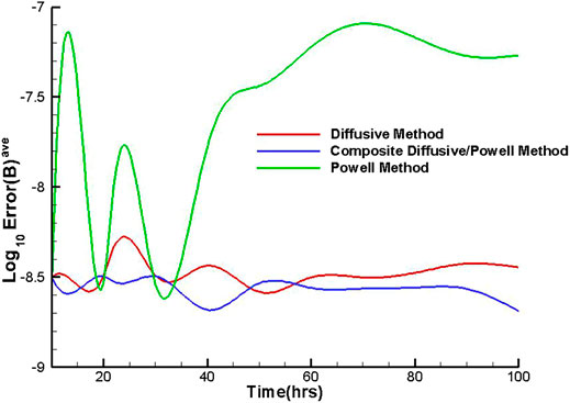
FIGURE 8. The temporal evolution of the Log₁₀Error(B)^ave from the three divergence cleaning methods.

Conclusions and Discussions

In this study, by using the 3D COIN-TVD MHD model, we simulate the solar wind in the coronal region, in which the divergence cleaning and coronal heating/acceleration methods are included. The volume heating method is an effective way for coronal heating, in which the parameters can be adjusted according to the WSA model in the simulation of the coronal solar wind. In the COIN-TVD MHD model, increasing the parameters $S_0$ and $Q_0$ of the energy and momentum source terms can make the solar wind accelerate more obviously.

For the divergence cleaning methods, here we choose the diffusive method, the Powell method and the composite diffusive/Powell method. We compared the numerical characteristics of the combination of each method for handling the divergence of the magnetic field and the COIN-TVD MHD model in the solar coronal simulation. The numerical results show that all of them can produce large-scale structured solar wind and reduce the divergence of the magnetic field more or less. The difference between the three divergence cleaning methods is summarized as follows:

1) The Powell method is relatively simple to apply. It only needs to add two items to the source term of the MHD equations. In this study, the Powell method can reduce the error of the relative magnetic field divergence, but it is less effective than the other two methods in dealing with magnetic divergence.

2) The diffusive method also has a good effect on reducing magnetic field divergence error in this study. It reduces the error of divergence by adding a source term in the induction equation and the $\nabla \cdot \mathit{B}$ error is diffused away by iterating ${\mathit{B}}^{k+1}={\mathit{B}}^k+\mu {\left(\Delta x\right)}^2\nabla \nabla \cdot {\mathit{B}}^k$. If it is coupled with different numerical schemes, the effects of controlling divergence error are different. In this study, the diffusive method is not as good as the composite diffusive/Powell method in controlling the divergence of the magnetic field, but better than the Powell method.

3) The composite diffusive/Powell method is a preliminary new try in this study, and it combines the Powell method and the diffusive method during the simulation. It has been proven that this composite method is the most efficient way to reduce the relative divergence errors among the three methods we used. Moreover, it also ensures the conservation of the MHD equations during the simulation.

In addition to the methods we mentioned, there are many other methods to simulate the coronal heating and the solar wind acceleration process and to control the divergence of the magnetic field. For example, both the Alfvén wave heating method and the turbulent heating method are effective for coronal heating. The Powell method can also company with other methods to control the magnetic divergence, which may be implemented in the future. Moreover, although these simulations are performed for the background solar corona, these methods can also be used for the simulation of CME initiation and propagation in the interplanetary space.

Data Availability Statement

The original contributions presented in the study are included in the article/supplementary files, further inquiries can be directed to the corresponding author/s.

Author Contributions

FS provided the thesis research topic, FS and YL provided the code for the three-dimensional solar wind numerical simulation. CL modified the code, ran the program code, and drew pictures based on the data. FS, CL, and MZ participated in the analysis of the results and the writing of the manuscript. XL modified the manuscript.

Funding

This work was jointly supported by the Strategic Priority Research Program of the Chinese Academy of Sciences, Grant no. XDB 41000000, National Natural Science Foundation of China (Grant nos 41774184 and 41974202), and State Key Laboratory of Special Research Fund Project.

Conflict of Interest

The authors declare that the research was conducted in the absence of any commercial or financial relationships that could be construed as a potential conflict of interest.

Publisher’s Note

All claims expressed in this article are solely those of the authors and do not necessarily represent those of their affiliated organizations, or those of the publisher, the editors and the reviewers. Any product that may be evaluated in this article, or claim that may be made by its manufacturer, is not guaranteed or endorsed by the publisher.

Acknowledgments

We acknowledge the use of synoptic magnetogram from the Global Oscillation Network Group (GONG). The numerical simulation of the model uses Tianhe-1A supercomputing machine.

References

1. Feng X, Wu ST, Wei F, Fan Q. A Class of Tvd Type Combined Numerical Scheme for Mhd Equations and its Application to Mhd Numerical Simulation. Chin J Space Sci (2002) 22(4):300–8. doi:10.3969/j.issn.0254-6124.2002.04.002

CrossRef Full Text | Google Scholar

2. Feng X, Wu ST, Wei F, Fan Q. A Class of TVD Type Combined Numerical Scheme for MHD Equations with a Survey about Numerical Methods in Solar Wind Simulations. Space Sci Rev (2003) 107:43–53. doi:10.1023/A:1025547016708

CrossRef Full Text | Google Scholar

3. Feng X, Xiang CQ, Zhong DK, Fan QL. A Comparative Study on 3-D Solar Wind Structure Observed by Ulysses and MHD Simulation. Chin Sci Bull (2005) 50:672–8. doi:10.1360/982004-293

CrossRef Full Text | Google Scholar

4. Shen F, Feng XS, Wang Y, Wu ST, Song WB, Guo JP, et al. Three-dimensional MHD Simulation of Two Coronal Mass Ejections' Propagation and Interaction Using a Successive Magnetized Plasma Blobs Model. J Geophys Res (2011) 116:A9. doi:10.1029/2011JA016584

CrossRef Full Text | Google Scholar

5. Shen F, Feng XS, Wu ST, Xiang CQ, Song WB. Three-dimensional MHD Simulation of the Evolution of the April 2000 CME Event and its Induced Shocks Using a Magnetized Plasma Blob Model. J Geophys Res (2011) 116:A4. doi:10.1029/2010JA015809

CrossRef Full Text | Google Scholar

6. Shen F, Wu ST, Feng X, Wu C-C. Acceleration and Deceleration of Coronal Mass Ejections during Propagation and Interaction. J Geophys Res (2012) 117:A11. doi:10.1029/2012JA017776

CrossRef Full Text | Google Scholar

7. Shen F, Shen C, Zhang J, Hess P, Wang Y, Feng X, et al. Evolution of the 12 July 2012 CME from the Sun to the Earth: Data-Constrained Three-Dimensional MHD Simulations. J Geophys Res Space Phys (2014) 119:7128–41. doi:10.1002/2014JA020365

CrossRef Full Text | Google Scholar

8. Shen F, Yang Z, Zhang J, Wei W, Feng X. Three-dimensional MHD Simulation of Solar Wind Using a New Boundary Treatment: Comparison with In Situ Data at Earth. ApJ (2018) 866:18. doi:10.3847/1538-4357/aad806

CrossRef Full Text | Google Scholar

9. Aschwanden MJ, Burlaga LF, Kaiser ML, Ng CK, Reames DV, Reiner MJ, et al. Theoretical Modeling for the Stereo mission. Space Sci Rev (2008) 136:565–604. doi:10.1007/s11214-006-9027-8

CrossRef Full Text | Google Scholar

10. Usmanov AV, Goldstein ML, Besser BP, Fritzer JM. A Global MHD Solar Wind Model with WKB Alfvén Waves: Comparison with Ulysses Data. J Geophys Res (2000) 105:12675–95. doi:10.1029/1999JA000233

CrossRef Full Text | Google Scholar

11. Zel'Dovich YB, Raizer YP, Hayes WD, Probstein RF, Gill SP. Physics of Shock Waves and High-Temperature Hydrodynamic Phenomena. J Appl Mech (1967)(4) 34. doi:10.1016/B978-0-12-395672-9.X5001-2

CrossRef Full Text | Google Scholar

12. Roussev II, Gombosi TI, Sokolov IV, Velli M, Manchester W, DeZeeuw DL, et al. A Three-Dimensional Model of the Solar Wind Incorporating Solar Magnetogram 15 Observations. Astrophysical J Lett (2003) L57(61):595. doi:10.1086/378878

CrossRef Full Text | Google Scholar

13. Cohen O, Sokolov IV, Roussev II, Arge CN, Manchester WB, Gombosi TI, et al. A Semiempirical Magnetohydrodynamical Model of the Solar Wind. ApJ (2006) 654:L163–L166. doi:10.1086/511154

CrossRef Full Text | Google Scholar

14. Cohen O, Sokolov IV, Roussev II, Gombosi TI. Validation of a Synoptic Solar Wind Model. J Geophys Res (2008) 113:A3. doi:10.1029/2007JA012797

CrossRef Full Text | Google Scholar

15. Suess ST, Poletto G, Wang A-H, Wu ST, Cuseri I. The Geometric Spreading of Coronal Plumes and Coronal Holes. Solar Phys (1998) 180:231–46. doi:10.1023/A:1005001618698

CrossRef Full Text | Google Scholar

16. Hansen KC, Gombosi TI, DeZeeuw DL, Groth CPT, Powell KG. A 3D Global MHD Simulation of Saturn's Magnetosphere. Adv Space Res (2000) 26:1681–90. doi:10.1016/S0273-1177(00)00078-8

CrossRef Full Text | Google Scholar

17. Parker EN. Dynamics of the Interplanetary Gas and Magnetic Fields. ApJ (1958) 128:664. doi:10.1086/146579

CrossRef Full Text | Google Scholar

18. Parker EN. Interplanetary Dynamical Processes. Phys Today (1963) 17(3):72.

Google Scholar

19. Parker EN. Dynamical Properties of Stellar Coronas and Stellar Winds. III. The Dynamics of Coronal Streamers. ApJ (1964) 139(8):690. doi:10.1086/147795

CrossRef Full Text | Google Scholar

20. Feng X, Yang L, Xiang C, Wu ST, Zhou Y, Zhong D. Three-dimensional Solarwindmodeling from the Sun to Earth by a Sip-Cese Mhd Model with a Six-Component Grid. ApJ (2010) 723:300–19. doi:10.1088/0004-637X/723/1/300

CrossRef Full Text | Google Scholar

21. Feng X, Zhang M, Zhou Y. A New Three-Dimensional Solar Wind Model in Spherical Coordinates with a Six-Component Grid. ApJS (2014) 214:6. doi:10.1088/0067-0049/214/1/6

CrossRef Full Text | Google Scholar

22. Dedner A, Kemm F, Kröner D, Munz C-D, Schnitzer T, Wesenberg M. Hyperbolic Divergence Cleaning for the MHD Equations. J Comput Phys (2002) 175:645–73. doi:10.1006/jcph.2001.6961

CrossRef Full Text | Google Scholar

23. Dedner A, Rohde C, Wesenberg M. A New Approach to Divergence Cleaning in Magnetohydrodynamic Simulations. In: TY Hou, and E Tadmor, editors. Hyperbolic Problems: Theory, Numerics, Applications. Berlin; Heidelberg: Spring-Verlag (2003). p. 509–18. doi:10.1007/978-3-642-55711-8-4710.1007/978-3-642-55711-8_47

CrossRef Full Text | Google Scholar

24. Susanto A, Ivan L, De Sterck H, Groth CPT. High-order central ENO Finite-Volume Scheme for Ideal MHD. J Comput Phys (2013) 250:141–64. doi:10.1016/j.jcp.2013.04.040

CrossRef Full Text | Google Scholar

25. Evans CR, Hawley JF. Simulation of Magnetohydrodynamic Flows - A Constrained Transport Method. ApJ (1988) 332:659–77. doi:10.1086/166684

CrossRef Full Text | Google Scholar

26. Ziegler U. A Semi-discrete central Scheme for Magnetohydrodynamics on Orthogonal-Curvilinear Grids. J Comput Phys (2011) 230:1035–63. doi:10.1016/j.jcp.2010.10.022

CrossRef Full Text | Google Scholar

27. Ziegler U. Block-Structured Adaptive Mesh Refinement on Curvilinear-Orthogonal Grids. SIAM J Sci Comput (2012) 34:C102–C121. doi:10.1137/110843940

CrossRef Full Text | Google Scholar

28. Brackbill JU, Barnes DC. The Effect of Nonzero ∇ · B on the Numerical Solution of the Magnetohydrodynamic Equations. J Comput Phys (1980) 35:426–30. doi:10.1016/0021-9991(80)90079-0

CrossRef Full Text | Google Scholar

29. Brandenburg A, Rädler KH, Rheinhardt M, Käpylä PJ. Magnetic Diffusivity Tensor and Dynamo Effects in Rotating and Shearing Turbulence. ApJ (2008) 676:740–51. doi:10.1086/527373

CrossRef Full Text | Google Scholar

30. Manabu Y, Kanako S, Yosuke M. Development of a Magnetohydrodynamic Simulation Code Satisfying the Solenoidal Magnetic Field Condition. Comput Phys Commun (2009) 180:1550–7. doi:10.1016/j.cpc.2009.04.010

CrossRef Full Text | Google Scholar

31. Powell KG, Roe PL, Linde TJ, Gombosi TI, De Zeeuw DL. A Solution-Adaptive Upwind Scheme for Ideal Magnetohydrodynamics. J Comput Phys (1999) 154:284–309. doi:10.1006/jcph.1999.6299

CrossRef Full Text | Google Scholar

32. Hayashi K. Magnetohydrodynamic Simulations of the Solar Corona and Solar Wind Using a Boundary Treatment to Limit Solar Wind Mass Flux. Astrophys J Suppl S (2005) 161:480–94. doi:10.1086/491791

CrossRef Full Text | Google Scholar

33. Feng X, Liu X, Xiang C, Li H, Wei F. A New MHD Model with a Rotated-Hybrid Scheme and Solenoidality-Preserving Approach. ApJ (2019) 871:226. doi:10.3847/1538-4357/aafacf

CrossRef Full Text | Google Scholar

34. Feng X, Zhang S, Xiang C, Yang L, Jiang C, Wu ST. A Hybrid Solar Wind Model of the Cese+hll Method with a Yin-Yang Overset Grid and an Amr Grid. ApJ (2011) 734:50. doi:10.1088/0004-637X/734/1/50

CrossRef Full Text | Google Scholar

35. Schatten KH, Wilcox JM, Ness NF. A Model of Interplanetary and Coronal Magnetic fields. Sol Phys (1969) 6(3):442–55. doi:10.1007/BF00146478

CrossRef Full Text | Google Scholar

36. Altschuler MD, Newkirk G. Magnetic fields and the Structure of the Solar corona. Solar Phys (1969) 9(1):131–49. doi:10.1007/BF00145734

CrossRef Full Text | Google Scholar

37. Lee CO, Arge CN, Odstrčil D, Millward G, Pizzo V, Quinn JM, et al. Ensemble Modeling of CME Propagation. Sol Phys (2013) 285:349–68. doi:10.1007/s11207-012-9980-1

CrossRef Full Text | Google Scholar

38. Moguen Y, Bruel P, Perrier V, Dick E. Non-reflective Inlet Conditions for the Calculation of Unsteady Turbulent Compressible Flows at Low Mach Number. Mech Industry (2014) 15(3):179–89. doi:10.1051/meca/2014027

CrossRef Full Text | Google Scholar

39. Nakamizo A, Tanaka T, Kubo Y, Kamei S, Shimazu H, Shinagawa H. Development of the 3-D MHD Model of the Solar corona-solar Wind Combining System. J Geophys Res (2009) 114:A7. doi:10.1029/2008JA013844

CrossRef Full Text | Google Scholar

40. Feng X, Jiang C, Xiang C, Zhao X, Wu ST. A Data-Driven Model for the Global Coronal Evolution. ApJ (2012) 758:62. doi:10.1088/0004-637X/758/1/62

CrossRef Full Text | Google Scholar

41. Feng X, Yang L, Xiang C, Jiang C, Ma X, Wu ST, et al. Validation of the 3D AMR SIP-CESE Solar Wind Model for Four Carrington Rotations. Sol Phys (2012) 279:207–29. doi:10.1007/s11207-012-9969-9

CrossRef Full Text | Google Scholar

42. Arge CN, Pizzo VJ. Improvement in the Prediction of Solar Wind Conditions Using Near-Real Time Solar Magnetic Field Updates. J Geophys Res (2000) 105(A5):10465–79. doi:10.1029/1999ja000262

CrossRef Full Text | Google Scholar

43. Arge CN, Luhmann JG, Odstrcil D, Schrijver CJ, Li Y. Stream Structure and Coronal Sources of the Solar Wind during the May 12th, 1997 CME. J Atmos Solar-Terrestrial Phys (2004) 66:1295–309. doi:10.1016/j.jastp.2004.03.018

CrossRef Full Text | Google Scholar

44. Suess ST, Wang A-H, Wu ST. Volumetric Heating in Coronal Streamers. J Geophys Res (1996) 101(A9):19957–66. doi:10.1029/96JA01458

CrossRef Full Text | Google Scholar

45. Yang L, Feng X, Xiang C, Zhang S, Wu ST. Simulation of the Unusual Solar Minimum with 3D SIP-CESE MHD Model by Comparison with Multi-Satellite Observations. Sol Phys (2011) 271:91–110. doi:10.1007/s11207-011-9785-7

CrossRef Full Text | Google Scholar

46. Spitzer L. Physics of Fully Ionized Gases. 2nd ed., 359. New York: Interscience (1962). 3559. doi:10.1126/science.139.3559.1045

CrossRef Full Text

47. Zhang M, Feng X. A Comparative Study of Divergence Cleaning Methods of Magnetic Field in the Solar Coronal Numerical Simulation. Front Astron Space Sci (2016) 3:6. doi:10.3389/fspas.2016.00006

CrossRef Full Text | Google Scholar

48. Pakmor R, Springel V. Simulations of Magnetic fields in Isolated Disc Galaxies. Month Notices R Astron Soc (2013) 432:176–93. doi:10.1093/mnras/stt428

CrossRef Full Text | Google Scholar

49. Gilchrist SA, Leka KD, Barnes G, Wheatland MS, DeRosa ML. On Measuring Divergence for Magnetic Field Modeling. ApJ (2020) 900:136. doi:10.3847/1538-4357/aba752

CrossRef Full Text | Google Scholar