Configuration of a Magnetic Cloud From Solar Orbiter and Wind Spacecraft In-situ Measurements

1 Introduction

Magnetic clouds (MCs) represent an important type of space plasma structures observed by in-situ spacecraft missions in the solar wind. They have been first identified in the in-situ spacecraft measurements of magnetic field and plasma parameters, and have been studied for decades, based on heliospheric mission datasets [1–4]. These include the earlier missions such as the Interplanetary Monitoring Platform (IMP), Helios, and Voyager missions. In later times, a number of NASA/ESA flagship missions, including Advanced Composition Explorer (ACE) [5], Wind [6], Ulysses [7], and Solar and TErrestrial RElations Observatory (STEREO) [8], have contributed greatly to the study of Solar-Terrestrial physics in general, and to the characterization of MC structures in particular. Generally speaking, the opportunities for one MC structure to be encountered by two or more spacecraft are rare, but when they do occur, it offers a unique opportunity for correlative and combined analysis between multiple spacecraft datasets (see references below).

A few such examples include an early study by [9] by using five spacecraft and the series of MC events in May 2007. During 19–23 May 2007, the newly launched twin STEREO spacecraft, Ahead and Behind, i.e., STEREO-A and B, respectively, were separated from Earth by $\sim 6^{\circ }$ and $\sim 3^{\circ }$, longitudinally, near 1 au. Therefore, the ACE, Wind, and STEREO spacecraft constellations observed a series of MC events, which enabled a number of correlative studies by using multi-spacecraft measurements [10–13]. Additionally, a number of studies took advantage of the rare occurrence of radial alignment of mostly two spacecraft separated in heliocentric distances, $r_h$, from the Sun. For example, Du et al. [14] studied an MC event and its evolution between the ACE and Ulysses spacecraft when they were separated radially by a distance of $\sim$ 4 au. They found that although the time-series data have evolved significantly between the two spacecraft, a flux rope configuration was still obtained at each spacecraft location and their magnetic field properties were compared. In this research topic collection, Song et al. [15] re-examined this event from the perspective of implications for elemental charge states in MCs. Lately, Davies et al. [16] analyzed an MC event detected in-situ by the Solar Orbiter (SO), Wind, and Bepi Colombo spacecraft in April 2020, and related to its solar source CME eruption by using the coronagraphic imaging observations from STEREO. We will re-examine this MC event by using the in-situ measurements from both SO and Wind spacecraft. We focus on the reconstruction of the magnetic field configurations and characterizations of the MC flux rope derived from the Wind spacecraft in-situ data. Quantitative comparison will be made with the magnetic field measurements along the projected SO spacecraft path across the same flux rope structure.

One commonly applied quantitative analysis method for MCs based on single-spacecraft in-situ data usually adopts the approach of an optimal fitting to an analytic solution, such as the well-known linear force-free field (LFFF) Lundquist solution [17], against the time series of magnetic field components within a selected interval. These solutions have limited one-dimensional (1D) spatial dependence, i.e., exhibit spatial variation in the radial dimension away from a central axis only. Recently we have improved the optimal fitting approach by extending the Lundquist solution to a quasi-three dimensional (3D) geometry [18, 19], based on the so-called Freidberg solution [20]. It represents a more general 3D configuration that can account for, to a greater degree, the significant variability in the in-situ measurements of MCs, such as the asymmetric magnetic field profile and sometimes the relatively large radial field component. An alternative two-dimensional (2D) method has also been applied to in-situ modeling of MCs, by employing the Grad-Shafranov (GS) equation, describing a two and a half dimensional (2–1/2D) configuration in quasi-static equilibrium [21–24]. This so-called GS reconstruction method is able to derive a 2D cross section of the structure traversed by a single spacecraft, yielding a complete quantitative characterization of the magnetic field configuration composed of nested cylindrical flux surfaces for a flux rope. Such a solution generally conforms to a cylindrical flux rope configuration with an arbitrary 2D cross section. The GS reconstruction method has been applied in a number of multi-spacecraft studies of MCs [see, e.g. [14, 25]], including the aforementioned MC events in May 2007 during the earlier stage of the STEREO mission. In addition, it has been widely applied to a variety of space plasma regimes with extended capability and additional improvement [26].

A new era has begun for solar and heliospheric physics with the launch of the Parker Solar Probe (PSP) [27] and the Solar Orbiter (SO) [28] missions. They will not only yield unprecedented new discoveries of never-before explored territories, but also provide two additional sets of in-situ measurements at different locations in the heliosphere. PSP will plunge closer to the Sun and reach a heliocentric distance below 0.1 au, and SO will provide highly anticipated measurements over a range of heliocentric distances and beyond the ecliptic plane. In this study, we examine one MC event detected during the month of April 2020 by both SO and Wind spacecraft when they were approximately aligned radially from the Sun, but separated by a radial distance of $\sim$0.2 au. We present an overview of the event in Section 2. The analysis results by using both the GS reconstruction and the optimal fitting methods are described in Section 3. In Section 4, we discuss the implications for the radial evolution of MCs under the condition of a nearly constant solar wind speed, based on the current event study results. We then summarize the results from this event study in the last section.

2 Event Overview

The SO mission observed its first ICME event on April 19, 2020 (day of year, DOY 110) at a heliocentric distance $\sim$0.81 au near the Sun-Earth line [16, 29]. As summarized in [16], the ICME complex arrived at SO at 05:06 UT, as marked by an interplanetary shock, and followed by a “magnetic obstacle” 3.88 h later, which may embody a flux rope structure, and lasted for about 24 h. The Wind spacecraft subsequently observed the same structures about 1 day later. Figures 1A,C show the in situ measurements from the spacecraft Wind and SO (magnetic field only [30]), respectively. Figure 1B shows the relative locations of a number of objects of interest including SO and Earth (Wind) on the X-Y plane of the Earth Ecliptic (HEE) coordinate system. Relative to Wind, SO was offset from the Sun-Earth (Wind) line by about 4.02° to the East, while it was North of the ecliptic plane with a latitude of about 1.22° [16].

FIGURE 1

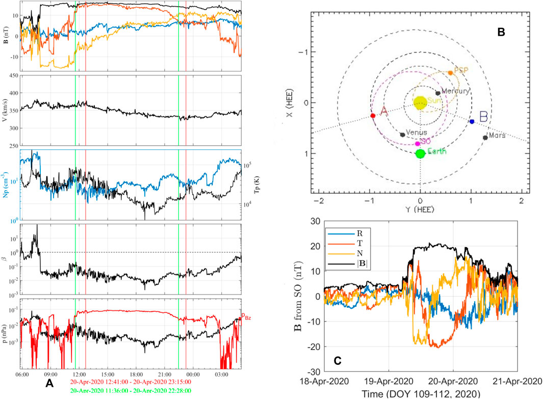
FIGURE 1. (A) Time series data from Wind spacecraft (from top to bottom panels) the magnetic field components in GSE-X (blue), Y (red), and Z (gold) coordinates and the magnitude (black), the solar wind speed, the proton number density (blue; left axis) and temperature (black; right axis), the proton β, and the proton plasma pressure and the axial magnetic pressure (red). Two sets of vertical lines mark the intervals for the GS reconstruction (green) and the optimal fitting to the Freidberg solution (red), respectively, and are denoted beneath the last panel. (B) The multiple spacecraft and planets locations around April 20, 2020 in the ecliptic plane (courtesy of the STEREO Science Center). (C) The corresponding SO magnetic field measurements in the RTN coordinates (see legend).

In Figure 1A, two intervals are marked for the subsequent analysis of the ICME/MC flux rope structure via the GS reconstruction method (between 11:36 and 22:28 UT) and the optimal 3D Freidberg solution fitting approach (between 12:41 and 23:15 UT) on April 20, 2020. The in-situ measurements enclosed by the vertical lines indicate clear signatures for an MC: 1) elevated magnetic field magnitude, 2) relatively smooth rotation in field components (i.e., mainly the GSE-Z component varying from negative to positive values), and 3) depressed proton temperature and β value. The corresponding measurements of magnetic field components at SO show similar features with slightly enhanced magnetic field magnitude. The plasma measurements were not available during these earlier time periods of the mission [16]. In particular, the rotation in the N component of the magnetic field at SO corresponds well to the rotation in the GSE-Z component at Wind, while the East-West components (along T and the GSE-Y directions) are approximately reversed. For a typical cylindrical flux rope configuration crossed by a single spacecraft, the magnetic field component with a uni-polar pattern usually corresponds to the field component along the axis of the flux rope, while the change in the north-south or east-west component usually indicates the rotation of the transverse field about the axis. Therefore these signatures, for this particular MC event, hint at a flux rope configuration lying near the ecliptic with the axial direction pointing eastward (positive GSE-Y component, aligned with the thumb of the left hand) with respect to the Sun and with a left-handed chirality (the handedness; GSE-Z component rotating from southward to northward direction, aligned with the other four fingers). Given the difference in the magnetic field magnitude and a 1-day time delay consistent with the radial separation distance between SO and Wind [16], it is plausible to consider an evolution between the two spacecraft as well as the spatial variation, assuming that the two spacecraft crossed the same structure along different paths mainly due to their longitudinal separation. In what follows, we present our analysis results and discuss the interpretations.

3 Methods and Results

We have developed and applied both 2D and 3D flux rope models to in-situ spacecraft measurements of MCs. The 2D model is based on the Grad-Shafranov (GS) equation and is able to derive a 2D cylindrical configuration with nested flux surfaces of arbitrary cross section shape [see, e.g. [26]]. The 3D model is based on a more general LFFF formulation, the so-called Freidberg solution [20], and accounts for a greater deal of variability in the in-situ data through a rigorous ${\chi }^2$ optimal fitting approach. This approach was recently developed and described in [18, 19]. Both methods can yield a set of parameters characterizing the geometrical and physical properties of the structure, including the axial orientation in space, the handedness (i.e., chirality, sign of magnetic helicity), and the axial magnetic flux content (sum of axial flux over a cross-section area), for a flux rope configuration. We apply both methods to the Wind spacecraft data of the MC intervals marked in Figure 1A, and cross-check with the corresponding magnetic field measurements along the separate SO spacecraft path across the same structure.

3.1 Grad-Shafranov Reconstruction Results

The GS reconstruction utilizes the spacecraft measurements of magnetic field $\mathit{B}$ and solar wind velocity $\mathit{V}$, and additional plasma parameters as initial conditions to solve the scalar GS equation, which governs the 2–1/2D magnetic field configuration across the cross section plane perpendicular to the z axis with $B_z\ne 0$ and $\partial /\partial z\approx 0$. The solution to the GS equation is obtained in the form of a 2D magnetic flux function $A\left(x,y\right)$, which fully characterizes the three components of the magnetic field especially including the axial field $B_z\left(A\right)$, among other quantities being single-variable functions of A. Figure 2A shows the data points along the Wind spacecraft path across the MC interval, and the functional form for $P_t\left(A\right)$ = $p+B_z^2/2{\mu }_0$, the sum of the plasma pressure and the axial magnetic pressure. Each quantity is a single-variable function of A as required by the GS equation. An optimal z axis orientation is found for which the requirement of $P_t\left(A\right)$ being single-valued is best satisfied [for details, see, 23]. For this case, the z axis orientation is found to be $\left(\delta ,\varphi \right)=\left(\mathrm{79,96}\right)\pm \left(\mathrm{4,9}\right)$¹ degrees, with uncertainties estimated by error propagation [24]. Then these functions, especially the fitted function $P_t\left(A\right)$, are used to solve the GS equation and obtain a cross section map of the 2D magnetic field structure given in Figure 2B for this event. It shows a flux rope configuration with distinct nested flux surfaces (iso-surfaces or contours of A), on which the field lines are winding along the z dimension and the axial field $B_z$ remains the same on each surface. The left-handedness (negative chirality) is readily seen from this cross section map, by pointing the thumb of the left hand upward in the positive $B_z$ direction, while wrapping the other four fingers around the direction marked by the white arrows along $y=0$. The center of the flux rope defined by the location of the maximum $B_z$ value appears to be away from the spacecraft path at $y=0$ in this case.

FIGURE 2

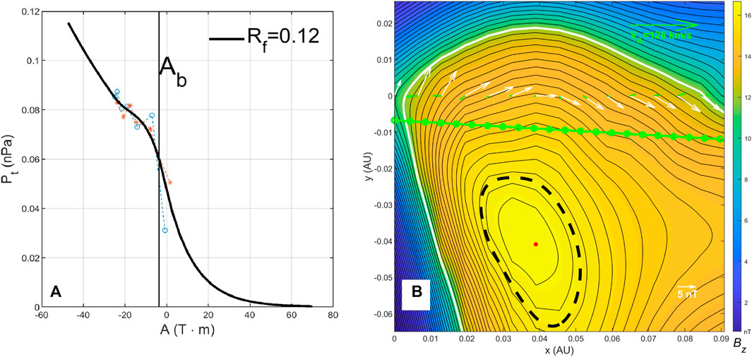
FIGURE 2. (A) The $P_t$ versus A data (symbols) along the Wind spacecraft path, and the fitted $P_t\left(A\right)$ curve (thick black curve) with the corresponding fitting residue $R_f$ denoted. The vertical line marks the boundary defined by $A=A_b$, (B) The cross section map from the GS reconstruction for the MC interval marked in Figure 1. The black contours are the iso-surfaces of $A\left(x,y\right)$, and the filled color contours indicate the axial field $B_z\left(A\right)$ with scales given by the colorbar. The Wind spacecraft path is projected along $y=0$ with white (green) arrows representing the measured transverse magnetic field (remaining flow) vectors. A reference vector proportional in magnitude for each set is provided, respectively, with the white reference vector in the lower right of magnitude 5 nT and the green reference vector of the magnitude of the average Alfvén speed in the top right. The SO spacecraft path is projected onto the same map as the green line with green circles. The thick dashed contour line highlights the outermost closed loop surrounding the center marked by the red dot where $B_z$ reaches the maximum $B_{z0}$.

This is a typical rendering of the GS reconstruction result as viewed down the z axis such that the flux surfaces (contours of A) are projected onto the cross-section plane as closed loops surrounding the center for a flux rope configuration. The axial magnetic field usually reaches the maximum at the center and decreases monotonically toward the outer boundary. Along the spacecraft path at $y=0$, the observed transverse magnetic field vectors are tangential to the contours. It is also indicated that the remaining flow (green vectors along $y=0$; see also below) as viewed in the frame moving with the flux rope structure is negligible compared with the average Alfvén speed (denoted in the top right-hand corner of magnitude 126 km/s). The effect associated with the inertial force in the magnetohydrodynamics (MHD) framework is assessed via the de Hoffmann-Teller (HT) analysis [see, e.g. [18]]. Figure 3 shows the HT analysis result for this MC interval, in terms of the Walén plot, yielding a slope 0.021 of the regression line. This indicates a negligible ratio between the remaining flow $\mathit{V}-{\mathit{V}}_{HT}$ and the local Alfvén velocity. Thus a quasi-static equilibrium as dictated by the GS equation in the HT frame moving with frame velocity ${\mathit{V}}_{HT}$ is approximately satisfied. For this event, since the SO spacecraft crossed the same structure at a close separation distance but at an earlier time, it is useful to project the SO path onto the cross section map generated by the Wind in-situ measurements, as indicated by the green line with circles in Figure 2B. We will further discuss the implications for the radial evolution between SO and Wind in Section 4.

FIGURE 3

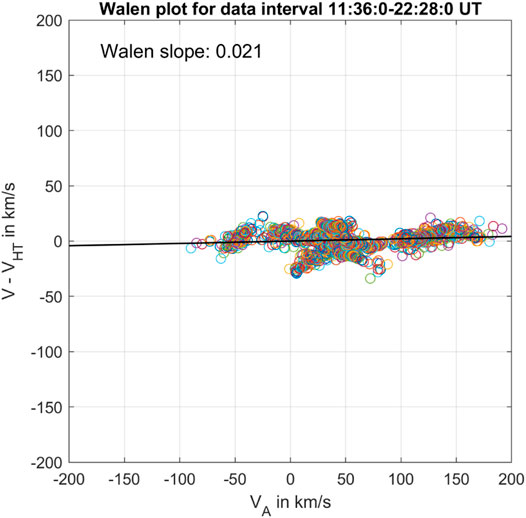
FIGURE 3. The Walén plot for the MC interval at Wind for which the GS reconstruction is applied. The HT analysis yields an HT frame velocity [−346.52, −10.81, 21.10] km/s, in the GSE coordinates. The slope of the regression line shown is denoted the Walén slope.

It is also informative to illustrate the magnetic field configuration in the perspective view toward the Sun with both Wind and SO spacecraft locations marked in Figure 4. This provides a direct 3D view toward the Sun (located at the same position as Wind in this view but at a distance 1 au away) along the Sun-Earth line. It is seen that the reconstructed flux rope structure based on the Wind in-situ data along its path shows selected spiral field lines with arbitrary colors winding around a central axis represented by the red straight field line, along the z axis direction, pointing approximately horizontally to the East with both Wind and SO spacecraft passing beneath the center of the flux rope, and separated mostly in the East-West direction. With the 2D reconstruction result from the Wind spacecraft, it enables a direct comparison between the derived magnetic field components along the SO spacecraft path, as shown in Figure 2B, and the actual measured ones returned by the spacecraft. Figure 5 shows such comparison of the three magnetic field components in the SO centered RTN coordinates. Figure 5A shows the component-wise time series within the MC interval at SO, while Figure 5B shows the corresponding one-to-one correlation plot, yielding a correlation coefficient $cc=0.95$, for all three components combined. When the correlation coefficients are computed separately for each component, they yield $c{c}_R=0.65$, $c{c}_T=0.12$, and $c{c}_N=0.95$, respectively, as denoted in Figure 5B.

FIGURE 4

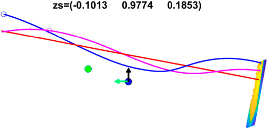
FIGURE 4. The 3D view toward the Sun (along the +GSE-X direction) of the selected field lines (with arbitrary colors) from the GS reconstruction result corresponding to Figure 2. The unit vectors of the GSE-Y and Z coordinates are denoted in green and black arrows, respectively. The cross section as seen in Figure 2B is shown to the right where the field lines originate and spiral along the z axis. The red straight field line originates from the center of the flux rope as marked in Figure 2B. The spacecraft locations of Wind and SO are marked by the blue and green dots, respectively. The z axis direction is denoted on top in the GSE coordinates.

FIGURE 5

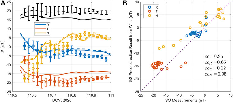
FIGURE 5. (A) The comparison between the derived magnetic field components (solid curves) based on the GS reconstruction result from Wind in Figure 2, and the actual measurements (circles and error bars), along the SO spacecraft path. The field magnitude is in black. (B) The corresponding component-wise one-to-one scatter plot with the correlation coefficients between the two sets for all three components, $cc$, and each individual component are denoted. The dashed line marks the one-to-one diagonal line. The dashed curves in (A) represent an alternative estimate/adjustment based on an argument of the $1/r_h$ dependence of the axial field.

One main discrepancy is the underestimated magnitude of the $B_T$ component. If one assumes the conservation of axial magnetic flux, it can be established $B_z\propto 1/r_h$ (i.e., inversely proportional to the heliocentric distance, $r_h$) with the additional supporting evidence of negligible inertial force provided by, e.g., the HT analysis. When this is the case, the dependence of the cross-section area becomes $\propto r_h$, considering largely the angular expansion but little expansion in the radial dimension, for a flux rope configuration with a z axis orientation nearly perpendicular to the radial direction. The so-called Walén slope as shown in Figure 3 signifies the relative importance of the inertial force, including the effect of radial expansion, to the Lorentz force in an MHD equilibrium. A small Walén slope magnitude is thus generally a prerequisite condition for the GS reconstruction and the subsequent optimal fitting approach [18], when they are all based on an approximate magnetohydrostatic equilibrium, sometimes with even stricter additional condition of being force-free. An adjustment based on the argument of the $1/r_h$ dependence of the axial field can be made to the model output at SO location, as shown in Figure 5A by the dashed curves. This yields a correlation coefficient (between the dashed curves and circles) $cc\prime =0.94$, and correspondingly, $cc{\text{′}}_R=0.65$, $cc{\text{′}}_T=0.23$, and $cc{\text{′}}_N=0.95$, although visually they appear to have improved agreement, especially in the $B_T$ component and the magnitude. We defer additional discussions regarding the radial evolution of MC to Section 4.

3.2 A Quasi-3D Configuration Based on the Freidberg Solution

We also apply an optimal fitting approach based on the quasi-3D Freidberg solution to the MC interval denoted in Figure 1A. For this interval, an HT frame velocity is obtained ${\mathit{V}}_{HT}=\left[-340.95,-4.16,22.24\right]$ km/s, in the GSE coordinates, with the corresponding Walén slope −0.0262. The average proton β is 0.023. The three magnetic field components of the Freidberg solution in a local cylindrical coordinates $\left(r,\theta ,z\right)$ are given in or by [20], each with dependence on all three dimensions,

$\frac{B_z\left(\mathit{r}\right)}{B_{z0}}=J_0\left(\mu r\right)+C{J}_1\left(\alpha r\right)\cos \left(\theta +kz\right)(1)$

$\frac{B_{\theta }\left(\mathit{r}\right)}{B_{z0}}=J_1\left(\mu r\right)-\frac{C}{\alpha }\left[\mu J{\prime }_1\left(\alpha r\right)+\frac{k}{\alpha r}{J}_1\left(\alpha r\right)\right]\cos \left(\theta +kz\right)(2)$

$\frac{B_r\left(\mathit{r}\right)}{B_{z0}}=-\frac{C}{\alpha }\left[kJ{\prime }_1\left(\alpha r\right)+\frac{\mu }{\alpha r}{J}_1\left(\alpha r\right)\right]\sin \left(\theta +kz\right)(3)$

Here the solution involves the Bessel’s functions of the first kind, $J_0$ and $J_1$. A set of free parameters includes mainly C, μ (the force-free constant, sign of μ representing chirality), and k, and additional geometrical parameters accounting for the arbitrary orientation and location of the solution domain relative to the spacecraft path. The parameter $B_{z0}$ is pre-determined as the maximum absolute value among all measured magnetic field components over the analysis interval and $\alpha =\sqrt{{\mu }^2-k^2}$. It is clearly seen that for $C\equiv 0$, the solution reduces to the 1D Lundquist solution with only r dependence.

An optimal fitting approach based on ${\chi }^2$ minimization with uncertainty estimates derived from in-situ spacecraft measurements was devised and applied to a few MC intervals [18, 19]. The results of minimum reduced ${\chi }^2\mathrm{\lesssim }1$ were obtained in terms of the evaluation of the deviation between the model output from the Freidberg solution and the corresponding spacecraft measurements of the magnetic field components along a single-spacecraft path across the structure. Detailed descriptions of the fitting procedures and comparison of results with the GS reconstruction output and multiple spacecraft measurements are presented in [18]. We apply this newly developed approach to the Wind spacecraft data and obtain an optima fitting result as shown in Figure 6. The minimum reduced ${\chi }^2\approx 1.7$ is obtained with associated accumulative probability $Q\approx 0.001$, an indication of the quality of the goodness-of-fit, marginally considered acceptable (for $Q\mathrm{\gtrsim }0.001$) [31]. In addition, the error estimates on the fitted parameters can be obtained via the standard evaluation of confidence limits applicable to such ${\chi }^2$ minimization as described in [31]. For example, the z axis orientation is found to be $\left(\delta ,\varphi \right)$=(60,90)$\pm \left(\mathrm{7,9}\right)$ degrees with 90% confidence limits. We present the other parameters in Section 5.

FIGURE 6

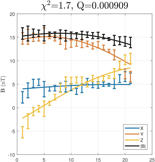
FIGURE 6. The optimal fitting result to the Freidberg solution for the MC interval marked in Figure 1A. The Wind spacecraft measurements of the magnetic field with uncertainty estimates are shown as error bars, while the corresponding analytic solution is given by solid curves (see legend). The horizontal axis is the integral index of the data points.

When compared with the GS reconstruction result, the significant distinction of this configuration represented by the Freidberg solution is the 3D nature, not present in any 2D configurations. There no longer exists distinctive 2D flux surfaces, and the field lines exhibit more general 3D features, not lying on discernable individual flux surfaces. Figure 7A demonstrates one cross section perpendicular to the z axis. The transverse field vectors are not tangential to the contours of $B_z$. There is no translation symmetry in the z dimension. To further illustrate this feature, Figure 7B shows the same view, but with a bundle of field lines drawn in orange color and originating from the bottom plane. No distinctive nested loops (flux surfaces) are seen. As a result, there does not exist a single central field line that is straight along z. Figure 8 is the same bundle of field lines viewed from the perspective of the Wind spacecraft toward the Sun. The flux bundle possesses an overall winding along the z dimension, likely related to the topological feature of writhe, giving rise to the 3D feature seen. It also contributes to the individual field line twist, which can be evaluated by the means used for the topological analysis of solar active region magnetic field [e.g. [32]]. The SO spacecraft appears to cross the flux rope bundle mostly to the East of the Wind spacecraft path, apart from a nominal time delay due to the radial separation. Figure 9 shows the comparison in a format similar to Figure 5, but for the optimal fitting result of the Freidberg solution to the Wind spacecraft data. The correlation coefficient between the field components from the optimal Freidberg solution and those from the actual measurements along the SO spacecraft path is $cc=0.96$ (additionally $c{c}_R=0.62$, $c{c}_T=0.57$, and $c{c}_N=0.92$). The combined correlation coefficient $cc$ remains the same if adjustments are made as represented by the dashed curves in Figure 9A, while correspondingly, the correlation between each individual component becomes $cc{\text{′}}_R=0.66$, $cc{\text{′}}_T=0.63$, and $cc{\text{′}}_N=0.92$, based on the argument of solely angular expansion to be discussed in the next section.

FIGURE 7

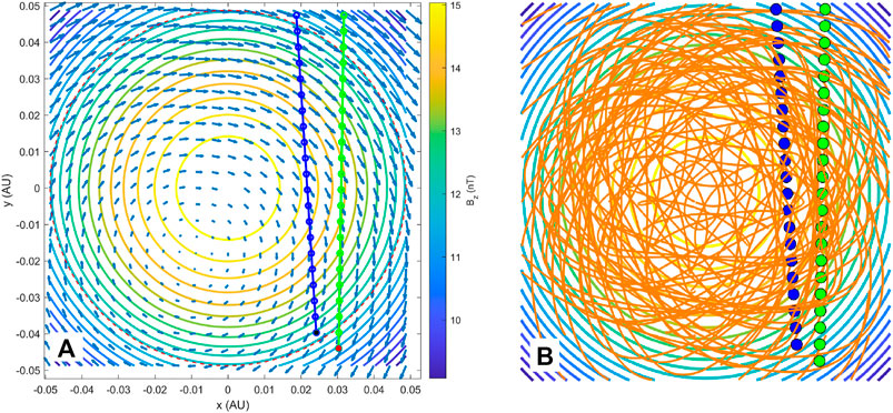
FIGURE 7. (A) One cross section of the optimal Freidberg solution where the colored contours represent $B_z$ distribution and arrows represent the transverse field components. The Wind and SO spacecraft paths are shown by the blue and green lines with dots, respectively. (B) The same view and contour lines for $B_z$ as (A). The orange lines are the field lines originating from the cross section plane, and viewed down the z axis.

FIGURE 8

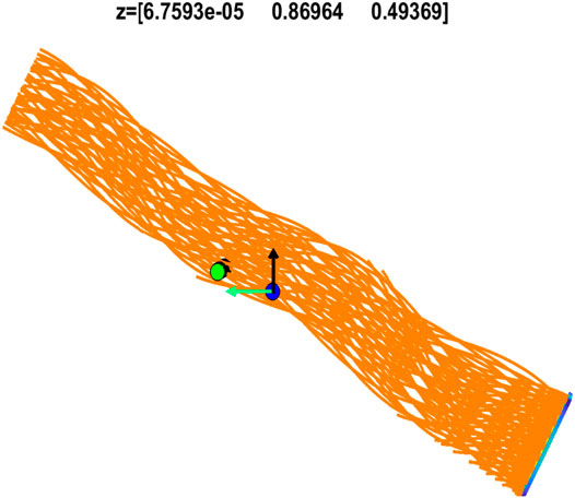
FIGURE 8. The 3D view of the field lines or the flux bundle of the Freidberg solution given in Figure 7B, from the same viewpoint and in the same format as Figure 4. The z axis orientation and the locations of Wind (blue dot) and SO (green dot) spacecraft are also marked.

FIGURE 9

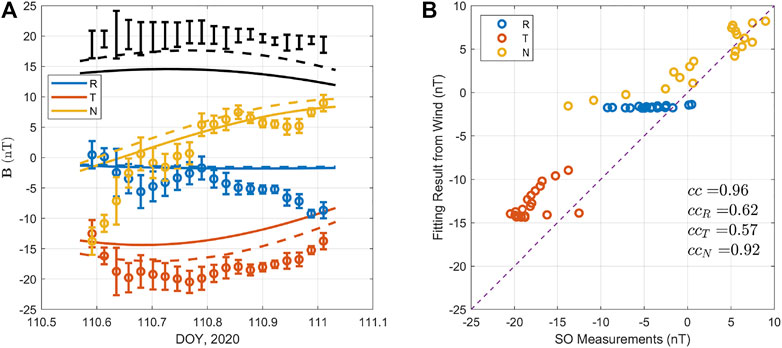
FIGURE 9. The comparison between the derived magnetic field components based on the optimal Freidberg solution fit to Wind spacecraft data, and the actual measurements, along the SO spacecraft path across the solution domain. Format is the same as Figure 5.

4 Discussion

We lay out, briefly, a consideration for the radial evolution of the MC, given the difference in the average magnetic field magnitude between SO and Wind during the MC interval, which can be partially accounted for by the spatial variations [see, also [16]]. Because the solar wind flow speed at Wind shows little variation, the expansion in the radial direction may be negligible for this event (also justified by the small Walén slope as shown in Figure 3). Therefore by assuming conservation of axial magnetic flux content and a constant angular extent of the MC flux rope cross section, $\text{ΔΘ}$, the following relation is assumed to be approximately satisfied,

$\langle B_z\rangle \Delta r_h\cdot r_h\Delta \Theta \sim {\Phi }_z\approx Const.(4)$

Here the average axial field $\langle B_z\rangle$ is obtained over the cross-section area of the flux rope, which is approximated by the product $\text{Δ}{r}_h\cdot r_h\text{ΔΘ}$. The cross-section length scale $\text{Δ}{r}_h$ is approximately constant if there is little change in the solar wind speed such that any inertial effect including expansion can be omitted (again as judged by the Walén slope). Then, it follows that the average axial field $\langle B_z\rangle$ or approximately $B_{z0}$ changes proportionally with $r_h^{-1}$. This seems to be true for this particular MC event (Table 1), and also consistent with [16]. Specifically, they found that the radial change of the mean MC field strength follows the dependence $\propto r_h^{-1.12\pm 0.14}$. They also concluded that this MC flux rope was not likely undergoing “self-similar or cylindrically symmetric expansion.” For this event, from Eq. 4 and Table 1, it is derived $\langle B_z\rangle \approx 15\mathrm{nT}$ at 1 au. It should increase to about 18 nT at SO. From time-series data, the mean (maximum) total magnetic field strength at SO and Wind are 19 (21) nT and 15 (16) nT, respectively. It also has to be cautioned that all the reconstructions are based on single-point measurements. In order to further establish this type of relationship, more event studies are needed.

TABLE 1

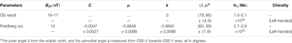
TABLE 1. Summary of geometrical and physical parameters for the MC based on Wind spacecraft measurements.

This study represents one step forward in the direction of quantifying how realistic MC model outputs are, based on one event study with available two-spacecraft in-situ observations. Future work would involve additional measurements and analysis based on remote-sensing observations, which will provide characterizations of solar source region (magnetic) properties of certain MC events to help further assess the fidelity of each model. The present implementations represent the best effort we have made in accounting for the variability in the in-situ measurements of MCs and proper error/uncertainty estimates of output parameters. Two models employed are deemed complementary and both are worth applying for individual event studies, as judged by the metrics, mainly, the combined correlation coefficients obtained from this two-spacecraft study with $cc>0.9$. In addition, the correlation coefficients for individual components are better for the Freidberg solution as compared to the GS result. When the radial evolution is considered as assumed by Eq. 4, the corresponding correlation coefficients for both methods slightly improve. There also seems to be a tendency that the Freidberg fitting method is more versatile which yields an acceptable solution when the GS reconstruction method fails [e.g., [19]]. Whether this holds for more number of events has yet to be explored.

5 Summary

In summary, we have examined one MC event in the solar wind by using the in-situ spacecraft measurements from both the Wind and SO missions located at heliocentric distances $\sim$1 and $\sim$0.8 au, respectively. Two spacecraft were largely aligned along the Sun-Earth line and nearly on the ecliptic plane, but SO was to the East of Wind with a longitudinal separation angle of $\sim$4°. The magnetic field measurements from both spacecraft show strong signatures of a magnetic flux rope configuration. In particular, the Wind plasma (not available from SO) and magnetic field measurements confirm the identification of an MC interval, which correlates with the corresponding magnetic field measurements at SO subject to a nominal time delay [see, also, [16]]. We apply both the 2D GS reconstruction method and the optimal quasi-3D Freidberg solution fitting method to the Wind spacecraft measurements and obtain the characterizations of the magnetic field topology at 1 au. A set of parameters from the analysis is summarized in Table 1. The error estimates of the parameters for the Freidberg solution are obtained at the 90% confidence limits, except for $B_{z0}$ and ${\text{Φ}}_z$. The former is pre-determined and fixed, while the latter is not a free fitting parameter. For the GS result, an uncertainty range for $B_{z0}$ is also obtained, while the parameters C, μ, and k are not applicable ($k=0$ for being 2D). Both methods yield a flux rope configuration with left-handed chirality (“$-$”) and their axial directions are oriented mainly along the West-East direction, with inclination angles relative to the ecliptic plane, about 11 and 30°, respectively. The axial magnetic flux content is 1.5–2.1$\times {10}^{20}$ Mx, and 2.7–2.8$\times {10}^{20}$ Mx, respectively, as indirectly derived from the model outputs, taking into account the uncertainties. Although the lack of plasma data from SO prohibits the same types of rigorous analysis at SO, we use the available magnetic field measurements at SO to correlate with the corresponding model outputs from the aforementioned quantitative analysis based on the Wind spacecraft data. This becomes feasible for this event study when the two spacecraft were positioned with an appropriate separation distance. We conclude that both spacecraft crossed the same structure exhibiting a flux rope configuration, as characterized by the set of parameters summarized above. Such an interpretation is supported by the analysis result that the combined correlation coefficients for the GS reconstruction result and the Freidberg solution fitting result are 0.95 and 0.96, respectively.

It is worth noting that as multi-spacecraft measurements become increasingly more available, as partially illustrated in Figure 1B, new and exciting multi-messenger science will be enabled by using multiple analysis tools. It is highly anticipated that the constellations of current and future missions will usher in new frontiers in heliophysics research.

Data Availability Statement

Publicly available datasets were analyzed in this study. This data can be found here: NASA CDAWeb: https://cdaweb.gsfc.nasa.gov/index.html/.

Author Contributions

QH carried out the analysis and wrote the draft of the manuscript. WH helped with the visualization of the analysis results. LZ obtained the time-series data from SO and participated in the interpretation of the results. EL helped with the analytic verification of the Freidberg solution.

Funding

Funding is provided, in part, by NASA Grant Nos. 80NSSC21K0003, 80NSSC19K0276, 80NSSC18K0622, 80NSSC17K0016, and NSF Grant Nos. AGS-1650854 and AGS-1954503, to The University of Alabama in Huntsville.

Conflict of Interest

The authors declare that the research was conducted in the absence of any commercial or financial relationships that could be construed as a potential conflict of interest.

Acknowledgments

WH and QH acknowledge NSO/NSF DKIST Ambassador program for support. The authors wish to thank Ms. Constance Hu for proofreading the manuscript. We thank the reviewers for useful comments that have helped improve the presentation of this manuscript.

Footnotes

¹The polar angle δ is from the ecliptic north, and the azimuthal angle ϕ is measured from GSE-X towards GSE-Y axes, all in degrees.

References

1. Burlaga LF. Magnetic Clouds and Force-free fields with Constant Alpha. J Geophys Res (1988) 93:7217–24. doi:10.1029/JA093iA07p07217

CrossRef Full Text | Google Scholar

2. Lepping RP, Jones JA, Burlaga LF. Magnetic Field Structure of Interplanetary Magnetic Clouds at 1 AU. J Geophys Res (1990) 95:11957–65. doi:10.1029/JA095iA08p11957

CrossRef Full Text | Google Scholar

3. Burlaga LF. Interplanetary Magnetohydrodynamics. In International Series in Astronomy and Astrophysics, 3. New York, NY: Oxford University Press (1995).

Google Scholar

4. Lepping RP, Burlaga LF, Szabo A, Ogilvie KW, Mish WH, Vassiliadis D, et al. The Wind Magnetic Cloud and Events of October 18-20, 1995: Interplanetary Properties and as Triggers for Geomagnetic Activity. J Geophys Res (1997) 102:14049–64. doi:10.1029/97JA00272

CrossRef Full Text | Google Scholar

5. Stone EC, Frandsen AM, Mewaldt RA, Christian ER, Margolies D, Ormes JF, et al. The Advanced Composition Explorer. Space Sci Rev (1998) 86:1–22. doi:10.1023/A:100508252623710.1007/978-94-011-4762-0_1

CrossRef Full Text | Google Scholar

6. Acuña MH, Ogilvie KW, Baker DN, Curtis SA, Fairfield DH, Mish WH. The Global Geospace Science Program and its Investigations. Space Sci Rev (1995) 71:5–21. doi:10.1007/BF00751323

CrossRef Full Text | Google Scholar

7. Longdon N. The Ulysses Data Book. A Summary of the Technical Elements of the Ulysses Spacecraft and its Scientific Payload (1990).Paris, France: European Space Agency.

8. Kaiser ML, Kucera TA, Davila JM, St Cyr OC, Guhathakurta M, Christian E. The STEREO Mission: An Introduction. Space Sci Rev (2008) 136:5–16. doi:10.1007/s11214-007-9277-0

CrossRef Full Text | Google Scholar

9. Burlaga L, Sittler E, Mariani F, Schwenn R. Magnetic Loop behind an Interplanetary Shock: Voyager, Helios, and Imp 8 Observations. J Geophys Res Space Phys (1981) 86:6673–84. doi:10.1029/JA086iA08p06673

CrossRef Full Text | Google Scholar

10. Kilpua EKJ, Liewer PC, Farrugia C, Luhmann JG, Möstl C, Li Y, et al. Multispacecraft Observations of Magnetic Clouds and Their Solar Origins between 19 and 23 May 2007. Solar Phys (2009) 254:325–44. doi:10.1007/s11207-008-9300-y

CrossRef Full Text | Google Scholar

11. Möstl C, Farrugia CJ, Miklenic C, Temmer M, Galvin AB, Luhmann JG, et al. Multispacecraft Recovery of a Magnetic Cloud and its Origin from Magnetic Reconnection on the Sun. J Geophys Res (Space Physics) (2009) 114:A04102. doi:10.1029/2008JA013657

CrossRef Full Text | Google Scholar

12. Möstl C, Farrugia CJ, Biernat HK, Leitner M, Kilpua EKJ, Galvin AB, et al. Optimized Grad - Shafranov Reconstruction of a Magnetic Cloud Using STEREO- Wind Observations. Solar Phys (2009) 256:427–41. doi:10.1007/s11207-009-9360-7

CrossRef Full Text | Google Scholar

13. Chollet EE, Mewaldt RA, Cummings AC, Gosling JT, Haggerty DK, Hu Q, et al. Multipoint Connectivity Analysis of the May 2007 Solar Energetic Particle Events. J Geophys Res Space Phys (2010) 115, A12106. doi:10.1029/2010JA015552

CrossRef Full Text | Google Scholar

14. Du D, Wang C, Hu Q. Propagation and Evolution of a Magnetic Cloud from ACE to Ulysses. J Geophys Res (Space Physics) (2007) 112:A09101. doi:10.1029/2007JA012482

CrossRef Full Text | Google Scholar

15. Song H, Hu Q, Cheng X, Zhang J, Li L, Zhao A, et al. The Inhomogeneity of Composition along the Magnetic Cloud Axis. Frontiers (2021) 9, 375. in press. doi:10.3389/fphy.2021.684345

CrossRef Full Text | Google Scholar

16. Davies EE, Möstl C, Owens MJ, Weiss A, Amerstorfer T, Hinterreiter J, et al. In Situ multi-spacecraft and Remote Imaging Observations of the First Cme Detected by Solar Orbiter and Bepicolombo. Astron Astrophysics (2021). doi:10.1051/0004-6361/202040113

CrossRef Full Text | Google Scholar

17. Lundquist S. On Force-free Solution. Ark Fys (1950) 2:361.

Google Scholar

18. Hu Q. Optimal Fitting of the Freidberg Solution to In Situ Spacecraft Measurements of Magnetic Clouds. Sol Phys (2021) 296, 101. Available at: https://arxiv.org/abs/2104.09352. doi:10.1007/s11207-021-01843-z

CrossRef Full Text | Google Scholar

19. Hu Q, He W, Qiu J, Vourlidas A, Zhu C. On the Quasi-Three Dimensional Configuration of Magnetic Clouds. Geophys Res Lett (2021) 48:e2020GL090630. doi:10.1029/2020GL090630

PubMed Abstract | CrossRef Full Text | Google Scholar

20. Freidberg JP. Ideal MHD. Cambridge, UK: Cambridge University Press (2014). p. 546–7.

21. Hau LN, Sonnerup BUÖ. Two-dimensional Coherent Structures in the Magnetopause: Recovery of Static Equilibria from Single-Spacecraft Data. J Geophys Res (1999) 104:6899–918. doi:10.1029/1999JA900002

CrossRef Full Text | Google Scholar

22. Hu Q, Sonnerup BUÖ. Reconstruction of Magnetic Flux Ropes in the Solar Wind. Geophys Res Lett (2001) 28:467–70. doi:10.1029/2000GL012232

CrossRef Full Text | Google Scholar

23. Hu Q, Sonnerup BUÖ. Reconstruction of Magnetic Clouds in the Solar Wind: Orientations and Configurations. J Geophys Res (Space Physics) (2002) 107:1142. doi:10.1029/2001JA000293

CrossRef Full Text | Google Scholar

24. Hu Q, Smith CW, Ness NF, Skoug RM. Multiple Flux Rope Magnetic Ejecta in the Solar Wind. J Geophys Res (Space Physics) (2004) 109:A03102. doi:10.1029/2003JA010101

CrossRef Full Text | Google Scholar

25. Hu Q, Smith CW, Ness NF, Skoug RM. On the Magnetic Topology of October/November 2003 Events. J Geophys Res (Space Physics) (2005) 110:A09S03. doi:10.1029/2004JA010886

CrossRef Full Text | Google Scholar

26. Hu Q. The Grad-Shafranov Reconstruction in Twenty Years: 1996 - 2016. Sci China Earth Sci (2017) 60:1466–94. doi:10.1007/s11430-017-9067-2

CrossRef Full Text | Google Scholar

27. Fox N, Velli M, Bale S, Decker R, Driesman A, Howard R, et al. The Solar Probe Plus mission: Humanity’s First Visit to Our star. Space Sci Rev (2016) 204:7–48. doi:10.1007/s11214-015-0211-6

CrossRef Full Text | Google Scholar

28. Müller D, St Cyr OC, Zouganelis I, Gilbert HR, Marsden R, Nieves-Chinchilla T, et al. The Solar Orbiter mission - Science Overview. A&A (2020) 642:A1. doi:10.1051/0004-6361/202038467

CrossRef Full Text | Google Scholar

29. Zhao LL, Zank GP, He JS, Telloni D, Hu Q, Li G, et al. Turbulence/wave Transmission at an ICME-Driven Shock Observed by Solar Orbiter and Wind. e-prints. arXiv (2021). arXiv:2102.03301.

30. Horbury TS, O’Brien H, Carrasco Blazquez I, Bendyk M, Brown P, Hudson R, et al. The Solar Orbiter Magnetometer. Astron Astrophys (2020) 642, A9. doi:10.1051/0004-6361/201937257

CrossRef Full Text | Google Scholar

31. Press WH, Teukolsky SA, Vetterling WT, Flannery BP. Numerical Recipes in C++ : The Art of Scientific Computing. New York: Cambridge Univ. Press (2007). 778. Available at: http://numerical.recipes/.

32. Liu R, Kliem B, Titov VS, Chen J, Wang Y, Wang H, et al. Structure, Stability, and Evolution of Magnetic Flux Ropes from the Perspective of Magnetic Twist. Astrophysical J (2016) 818:148. doi:10.3847/0004-637x/818/2/148

CrossRef Full Text | Google Scholar