Transverse and Quantum Localization of Light: A Review on Theory and Experiments

1 Introduction

Transverse localization (TL) is found in media in which the refractive index is randomly modulated only orthogonally to the direction of propagation. In these paraxial systems, Anderson localization (AL) sustains nondiffracting beams: confined light tubes showing many potential applications including fiber optics, quantum communication, and endoscopic imaging. In this review we will summarize recent advances in disordered optical fibers, in which confinement is obtained thanks to localization, discussing the advantages with respect to standard fibers. First we will report the latest experimental results on transverse Anderson localization: the migration of localized states due to nonlinearity, self-focusing, wavefront shaping in the localized regime, and the single-mode transport in disordered paraxial structures. This last result is particularly important as it bridges the physics of Anderson localization to the single-mode properties of optical fibers.

Then we will show how the traditional description of Anderson localization, which was based on the analogy to electrons in a random potential, turned out to be in error and led to the prediction of a localization length depending strongly on the wavelength of the light, which was not observed. We also report on the alternative correct theory, which relies on an analogy to acoustical waves in the presence of random elastic moduli. Regarding quantum aspects, we will report on how a single-photon state localized in some of its inner degrees of freedom could be an effective resource in quantum communication and cryptography, increasing both the amount of information loaded per single particle and the security and performance of protocols based on localized photon quanta. Finally, we will review the so-called random quantum walks in which the dynamics of a single particle moving on a lattice conditionally to the state of an ancillary degree of freedom display localization under certain conditions. A further aspect of AL of quantum particles is the behavior of the multiparticle interference and of the particle statistics in quantum walks. In the first proof-of-principle photonic experiments, AL has been observed in the two-photon wave function. In this scenario, it could be possible to simulate even the fermionic statistics by proper manipulation of two-photon entangled states generated by single-photon sources.

1.1 Modeling Transverse Localization: The Beginning

In the last decades, the idea that Anderson localization could be applied to electromagnetic waves [1, 2] has drawn the attention of the scientific community, stimulating experiments and conjectures. The excitement was further propelled by the following observation of the coherent backscattering cone (the so-called weak localization) [3–5]. Several experiments claimed strong localization of light in bulk media [6–8], but these results are still today strongly debated [9–12]. First Abdullaev in 1980 [13] and then De Raedt and coworkers in 1989 [14] proposed an alternative form of localization for light: the transverse localization. These authors described an optical system translationally invariant along the propagation direction of the waves, together with a refractive index varying randomly in the directions rectangular to it (transverse disorder). As usual in diffraction theory one can reduce the appropriate Helmholtz equation to a paraxial one [15, 16], which will be outlined in the following [14].

We start from the Helmholtz equation for the scalar field ϕ (r), which represents one of the components of the electric field E (r, t)

${\nabla }^2\varphi (\mathbf{r})+\frac{{\omega }^2}{c^2}{n}^2(x,y)\varphi (\mathbf{r})=0(1)$

where ω is 2π times the frequency, c is the vacuum light velocity, and r = [x, y, z]. In the case of spatial longitudinal invariant system, the function n(x, y) is the (transversely varying) refractive index. Due to the translation invariance in the z direction, the wave function can be represented as

$\varphi (\mathbf{r})=a(\mathbf{r})\exp (-i{k}_{0}z)(2)$

where a(r) is the envelope in z direction and describes the localization effects in (x, y) direction. k₀ = n₀ω/c = 2π/λ is the wavenumber in the medium. n₀ is the average refractive index in the disordered medium (disordered fiber), and λ is the wavelength in the medium. Equation 1 becomes

$-\frac{{\partial }^{2}a(\mathbf{r})}{\partial z^2}+2i{k}_0\frac{\partial a(\mathbf{r})}{\partial z}=\frac{{\partial }^{2}a(\mathbf{r})}{\partial x^2}+\frac{{\partial }^{2}a(\mathbf{r})}{\partial y^2}+k_0^2\left[\frac{n{(x,y)}^2-n_0^2}{n_0^2}\right]a(\mathbf{r}).(3)$

By introducing a transverse Laplace operator ${\nabla }_{\perp }^2=\frac{{\partial }^2}{\partial x^2}+\frac{{\partial }^2}{\partial y^2}$ and making the paraxial approximation [16]

$\left|\frac{{\partial }^{2}a(\mathbf{r})}{\partial z^2}\right|\ll 2k\left|\frac{\partial a(\mathbf{r})}{\partial z}\right|(4)$

Equation 3 becomes

$2i{k}_0\frac{\partial }{\partial z}a(x,y,z)=\left({\nabla }_{\perp }^2+U(x,y)\right)a(x,y,z).(5)$

where the potential is defined in terms of the spatially fluctuating refractive index:

$U(x,y)=k_0^2\left[\frac{n{(x,y)}^2-n_0^2}{n_0^2}\right]\approx 2k_0^2\frac{\mathrm{\Delta }n(x,y)}{n_0},(6)$

with Δn(x, y) = n(x, y) − n₀. Equation 5 is formally equivalent to the Schrödinger equation driving electron localization [17]. Here the z component mimics the time dependence in the Schrödinger equation and the index fluctuations mimic the random potential. In their seminal paper De Raedt et al. solved this equation numerically and obtained evidence for transverse Anderson localization for an index contrast of Δn = 0.25 and 0.5.

2 Experiments on Transverse Localization

The first papers on transverse localization were focused on theoretical modeling and numerical simulations. The experimental realization of the effect required more than a decade from the appearance of the paper of De Raedt et al. [14], because it required several technological advances on the fabrication side. The difficulty relies in the realization of the translationally invariant disorder in the z direction, which is particularly challenging at optical wavelengths, where it is needed to realize “paraxial defects,” i.e., invariance of the defect structures along the symmetry axis for sufficient length and size. The first successful approach was the “writing method” based on the application of the photo-refractive effect, which easily enables to produce z-invariant defect structures, employing Gaussian beams. On a second stage, the TL has been realized employing fiber-drawing technology, which enabled to produce longer structures, larger refractive index contrasts, and finally application-ready transverse-localized fibers. In the last stage, TL femtosecond direct laser writing was applied, which enabled the direct control of the defect positioning in order to investigate effects related to the disorder design. In the following, we will describe all this.

2.1 Early Experiments

The first experimental observation of TL (and actually one of the most unequivocal experimental manifestation of light localization) has been reported by Schwartz and coworkers [18] employing photo-refractive media. The authors employed the optical induction technique [19], to transform the intensity distribution of an array of parallel laser beams into a refractive-index distribution thanks to the nonlinear response of the glassy material. The distribution of the beam intensity is controlled with an interference mask, thus enabling the experimentalist to design the disorder configuration. The approach of Schwartz and coworkers induces a small refractive index contrast (Δn ∼ 10^–4) and a large disorder grain size (∼ 10 µm), thus the expected mean free path ℓ (the spatial length over which light propagation direction memory is lost) could be rather large. However, because the localization length, according to the scaling theory [20, 21] is proportional to $e^{k_{\perp }\ell }$, they argue that they deal with a very small perpendicular wavenumber k_⊥. The latter is the projection of the wavevector onto the x−y plane k_⊥ = k₀  sin θ, with θ being the incidence angle; see the sketch in Figure 1.

FIGURE 1

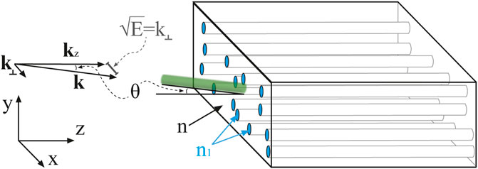
FIGURE 1. Sketch of transverse localization: sketch of the scattering structure and illumination for the realization of the TL. Light, in the form of a plane wave defined by the wavevector k, is impinging on the sample, with an azimuthal angle θ. The projection of the wavevector on the x-y plane (parallel to the fiber facet) k_⊥ and the projection of the wavevector on the propagation direction z (k_z) are reported, together with the spectral parameter $\sqrt{\left(\right.E}\left.\right)=k_{\perp }$ (see Section 3). The disordered system is typically consisting of a matrix of refractive index n containing “inclusions” with a different refractive index n₁. To work as “paraxial defects”, the defect structures with index n₁ should be precisely parallel to z.

The big advantage of the optical induction is the possibility to completely rearrange the refractive index distribution, with a simple and fast rewriting procedure. The possibility to perform experiments with several realizations of the disordered n(x, y) pattern enables to retrieve averaged-over-disorder quantities and this is an important aspect for verifying the presence of light localization. In particular, the authors of [22] demonstrated a dependence of the localization length on the degree of disorder, thus demonstrating TL.

2.2 Optical Fibers

In 2012, Arash Mafi and coworkers [18] demonstrated TL in an optical fiber, composed of polymer materials. They used a novel kind of fiber named disordered binary fibers (DBF), based on the random mixing of tens of thousands of polymer fibers of two types: poly-methyl-methacrylate (PMMA) and polystyrene (PS). The fibers were put together randomly and then thinned by applying a fiber-drawing tower.

By this procedure, homogenous fibers were realized with a realization of transverse disorder in the refractive index. The binary fiber approach provides several advantages: 1) the disordered refractive index distribution is permanent, 2) the refractive index mismatch between the two materials (Δn ∼ 0.1) has orders of magnitude higher than in the case of the photorefractive structures, and 3) the optical fibers are a mature technology ready for applications based on localization. Mafi and coworkers also fabricated glass optical fibers hosting transverse disorder and demonstrated TL therein [18]. The glass platform is extremely favorable for applications, providing very high refractive index contrast together with increased stability and lower absorption.

2.3 Image Transport

In-fiber implementation of the Anderson localization enables the propagation of localized beams with the transverse size comparable to that of cores of commercial single mode optical fibers. Thus a single disordered fiber with sufficient transverse extension can act as a coherent fiber bundle [23]. In [24] Mafi and coworkers demonstrated image transport through disordered optical fibers up to 5 cm. The transported image quality is comparable to or slightly better than the one obtainable with commercially available multicore image fibers, with disorder reducing the pixelation effect present in periodic structures and improved contrast. On the other hand, the imaging resolution is limited by the quality of the cleaving and polishing of the fiber tip, while the transport distance is limited by the optical attenuation and the residual longitudinal disorder resulting from the imperfect drawing process. In this sense, a glass-based disordered fiber, with a higher filling fraction and much lower losses, has the potential to further improve endoscopic disordered fibers.

2.4 Experimental Test of the Traditional Theory of Anderson Localization

The traditional theoretical description of Anderson localization of light, and, in particular, transverse Anderson localization [14, 18, 25] predicts a pronounced dependence of the localization length on the light wavelength. This is implied by the dependence of the potential U (x, y) in Eq. 5 on k₀ = 2π/λ

$2i{k}_0\frac{\partial }{\partial z}a(x,y,z)=\left({\nabla }_{\perp }^2+\underset{U(x,y)}{\underbrace{k_0^2\left[\frac{n{(x,y)}^2-n_0^2}{n_0^2}\right]}}\right)a(x,y,z).$

We call the traditional approach according to Eq. 5 the potential-type approach (PT). The authors of [26] investigated this effect experimentally (see a sketch of the setup in Figure 2A) in order to verify the validity of the current theory of Anderson localization of light. The experimental setup is shown in Figure 2. Figure 2B reports the localization length ξ versus the incident-laser wavelength: no dependence on the wavelength is retrieved in the range 0.55 ≤ λ ≤ 1 μm. This is in contrast to a simulation of Karbase et al. [25] of the same specimens, using Eq. 5, showing a strong dependence on the wavelength λ = 2π/k₀; see the dashed line in Figure 2. The reason for this discrepancy with the theoretical predictions will be fully explained in the following section. Here, we just sketch the essence of the findings of the authors of [26]:

1) In deriving the wave, Eq. 5, it has been tacitly assumed that the divergence of the electric field would be zero. In the presence of a spatially varying index of refraction, the divergence is, however, nonzero and is given by

${\nabla }_{\perp }\cdot \mathbf{E}=-\frac{1}{n^2(x,y)}\mathbf{E}\cdot {\nabla }_{\perp }{n}^2(x,y)\ne 0.(7)$

FIGURE 2

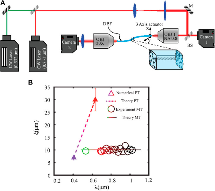
FIGURE 2. Probing the wavelength dependence of the average localization length. (A) Experimental setup: the probe beam is generated either by a tunable laser (tunability range 0.690 and 1.04 μm) or at a fixed wavelength (532 nm) laser. The back-reflected light is then visualized by the camera CCD1 through the beam-splitter (BS) to focus the beam at the fiber entrance. The piezo devices control the laser injection location. The transmitted light is collected by the objective OBJ2 and imaged on camera CCD2 with a magnification of ×50. Panel B reports the average localization length ξ versus wavelength λ for both numerically simulated and experimental data. Experimental data (open circles) are from [26] while numerical data, based on the approximate, traditional potential-type (PT) approach of Eq. 5 (full triangles and dashed line) are from [25]. The full line represents the prediction of our new, modulus-type approach (MT), which is exact [26].

Approximately neglecting this term leads to the strong dependence of the localization length on k₀, and, hence, on the laser wavelength (dashed line in Figure 2B) [14, 18, 25], at variance with the experimental findings (Figure 2B).

2) An alternative wave equation has been derived by the authors of [26], in which the electric modulus 1/n²(x, y) enters (“modulus-type,” MT), and which involves no approximation (except the paraxial one):

$2i{k}_0\frac{\partial }{\partial z}\mathit{b}(x,y,z)=-{\nabla }_{\perp }\times \frac{1}{n^2(x,y)}{\nabla }_{\perp }\times \mathit{b}(x,y,z).(8)$

here, $\mathit{b}(x,y,z)=e^{-i{k}_{0}z}\mathbf{B}(x,y,z)$ and B is the magnetic field. This wave equation does not predict any wavelength dependence of the average localization length (full line in Figure 2B), in agreement with the experimental data.

2.5 Nonlinearity in Disordered Optical Fibers

There is a relevant debate about the fact that nonlinearity [27, 28] may enhance disorder induced localization. The interplay between disorder and a nonlinear response may strongly modify the process of disordered induced wave trapping in TL. In particular in the case of nonlocality, while localization tends to reduce the intermode interactions, a nonlinear perturbation, extending beyond the region of the localized state, could eventually produce some kind of action at a distance. The first experimental evidence of nonlocality acting together with Anderson localization in an optical fiber has been shown in [29]. In that paper, the disordered fiber has been probed with a broadband laser beam, showing a distribution of sharp peaks in the transmittance, as expected from the “resonant” behavior of the disorder induced localized states [in Figure 3A we report the spectrum transmitted from the fiber (blue) compared to the probe spectrum (red)]. The first evidence is that the spatial shape of the localized states is strongly affected by energy probe beam power. This effect is reported in Figures 3B,C, where the localized state shape is reported as a function of the input power. The mode is seen to shrink when power is augmented. The presence of sharp peaks in the spectrum for all the power values confirms that the nonlinear action conserves the coherence of probe light.

FIGURE 3

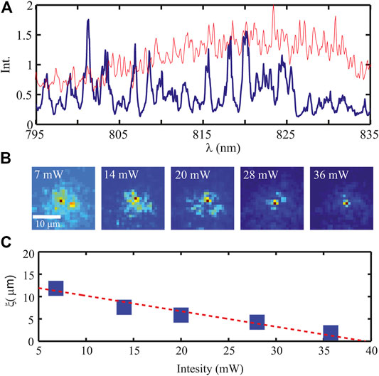
FIGURE 3. Localized states and nonlinearity. Panel (A) reports the spectrum (blue thick line) retrieved at the output of a disordered fiber (the collection area is 1 µm). The red thin line represents the source spectrum. Panel (B) reports the shape of the most intense mode (at ≃801 nm), for five values of the input power. Panel (C) shows localization length versus input intensity. All data are from [29].

This self-focusing results from the peculiar interaction between disorder and thermal nonlinearity. In general, the refractive index of a nonlinear optical material, varies with the optical intensity I as n = n₀ + Δn(x, y) + n₂I, where Δn(x, y) is the refractive index fluctuation due to disorder and n₂ represent the coefficient of the nonlinear perturbation. A positive n₂ coefficient results in a converging wave front that can potentially surpass the diffraction limit. Conversely, a negative value of n₂ produces a defocusing nonlinearity, thus the expansion of the beam. In plastic binary fibers, one expects the slow thermal nonlinearity to yield a negative n₂, thus defocusing. However, experimental measurements report instead a focusing nonlinearity. This unexpected effect is explained as follows [30]: if the refractive index reduction is more pronounced in one of the two constituent materials of the binary fiber, the refractive index mismatch may increase. Thus the overall refractive index reduction is compensated by a stronger index contrast, resulting in a smaller mean free path. This argument is not affected if we switch from the PT to the MT description, because according to both theories the mean-free path is inversely proportional to the index contrast, resulting effectively in a decrease of the localization length, as shown in Figure 3.

This effect makes a local and optical tunability of the localization length possible, enabling to drive the position of the localized states in a form of localization-mediated beam steering. The steering effect is reported in Figure 4. Figure 4A shows light reflected by the fiber input: the probe beam (green spot on the left) and the pump beam (red spot on the right). Figures 4B–D show the shape of the probe beam at the output as a function of the pump beam power. Here it is possible to note how much the probe beam is attracted towards the pump one. Figure 4E shows the distance of the probe beam center as a function of the input power.

FIGURE 4

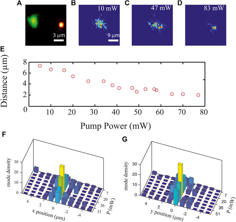
FIGURE 4. Light steering in the localization regime. Panel (A) shows the input of the DBF, showing the probe beam (green on the left) and the pump beam (red on the right). Panels (B–D) report the probe beam (pump light has been removed from the detector with a spectral filter) for several values of pump power. Panel E shows the distance between probe and pump beam versus the pump power. Panels (F–G) report the modes density along the X axis and Y axis (respectively) and for several pump powers. Data are from [29].

Nonlocality obviously works also when more than two modes are involved. The behavior of a group of localized modes is visualized in Figures 4F,G. Here we show (data from [29]) the mode density (number of localized modes per square µm) along the x and y axes at the output of a fiber. The mode density has been characterized for various values of the input power. The modes indeed appear to be attracting one another and then after a “collision” they start to diverge.

2.6 Localized States and “Single Modes”

The Anderson localization (AL) scenario typically comprises a disordered system supporting states which are strongly localized at different locations in space and at different energies [31]. These disorder-induced resonances have thus a poor or negligible spatial and spectral overlap, so that transverse energy transport is substantially slowed down.

While the majority of the studies on AL are focused on the measurement of transport-related quantities (such as diffusion or conductance [6–8, 21]), it is also interesting to study the properties of disorder-generated localized states. These light structures could be employed for energy storage [28, 32] or super-efficient lasing [33, 34]. Indeed localized states act exactly like a microresonator, with the difference that the resonance is sustained by a disordered structure instead of a regular one. In photonics, this kind of “lonely” structures are extensively employed in several fields: the most successful applications are in the field of fiber optics and laser resonators where they are named single-mode resonators or single-mode fibers. The principle of operation for both applications is very similar: they are resonant structures designed to host a single solution (typically the fundamental one) of the wave equation without (or with very small) losses.

In the case of disordered optical fibers, one may ask, to which extent a localized state operates as a single mode hosted in the core of single-mode fibers. This issue has been extensively studied in [35].

In contrast to multimode fibers, disordered binary fibers (DBF) show peculiar transmittance maps. The transmittance map is the total (integrated over the whole fiber tip output) intensity measured as a function of the injection location, and measured with the setup shown in Figure 5. Light from a CW laser is tightly focused into a spot of 0.7 µm diameter at the DBF input. The fiber input tip is sustained by a motorized actuator which enables to scan the injection location (r = [x, y]) along the input plane. The total transmittance T (r) is thus obtained by summing the whole intensity measured on the output plane (R = [X, Y]) by Camera 2. A typical transmittance map is reported in Figure 5A. It is possible to note that high transmittance locations (green spots) are appearing rather sparsely and surrounded by a sea of barely transmitting locations. These “hotspots” are the locations at which the input (which has a size much smaller than the localization length) couples efficiently to a transmission channel corresponding to a transversely localized state. The fact that the transmittance map is sparse should be thus a consequence of the fact that the coupling conditions are very “strict” (resonance bandwidth is very small) and thus coupling happens only at specific locations.

FIGURE 5

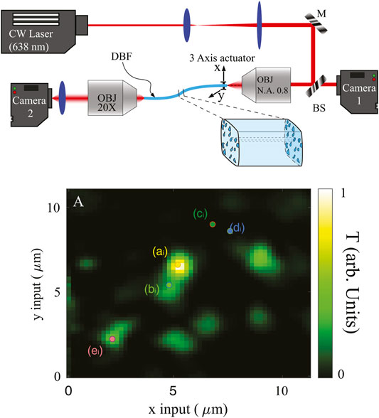
FIGURE 5. Probing single mode nature of localized states. The sketch reports a scheme of the experimental setup. Legend: CW laser, continuous wave laser; M, mirror; BS, beam-splitter; OBJ, objective; DBF, disordered binary fiber. Panel (A) reports the transmittance map in a 10 µm side field of view. Data are from [35].

Now it is interesting to further investigate the nature of these transmittance hotspots. The most accessible feature is the intensity profile measured at the fiber output: this is reported at Figure 6 for four different input locations. The input locations are identified by small colored dots labeled (a_ib_i, c_i, d_i) in Figure 5A. The intensity profiles in panels B and C of Figure 6B correspond to injection locations in the same hotspot and they produce two very similar output intensity profiles. On the other hand, two very close input locations lying in a barely transmitting area (panels C and D of Figure 6) produce two very different output intensity profiles. The intensity profile corresponding to a high efficient transmission channel is thus a fingerprint of the channel. In the same way the Gaussian profile going out from a single mode fiber is an indistinguishable signature for efficient coupling of a laser beam to the fundamental mode of the fiber’s core.

FIGURE 6

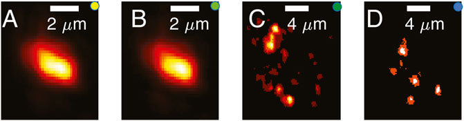
FIGURE 6. Mode fingerprints. Each panel reports the spatial profile of the intensity found for the correspondent location in Figure 5; i.e., panel (A) shows the fingerprint for location (a), (B) for location (b), etc. Data are from [35].

To verify this picture, one should observe where the mode’s fingerprint is found while scanning the input of the fiber. To perform this measurement systematically, the authors engineered a specialized observable that is the degree of similarity Q(r₁, r₂)

$Q(r_1,r_2)=\int I(R,r_1)I(R,r_2)dR,(9)$

normalized such that Q(r, r) = 1. The fingerprint of a transmission channel is the output intensity profile retrieved at the location of higher transmittance. So for the transmission channel located at a_i, it produces a Q-map Q(r_a, r₂) = ∫I (R, r_a)I (R, r₂)dR, where r_a corresponds to a location of higher intensity of the mode a_i. By computing Q(r_a, r₂) for all r₂ in the area of view, we retrieve the Q-map reported in Figure 7A. The white/bluish area (where Q ≃ 1) corresponds to the dwelling area of the mode: the set of input locations from which the mode can be activated. The dwelling area is very sharp, meaning that when the mode is activated, no other modes (which would modify the fingerprint and immediately lower the Q) are activated.

FIGURE 7

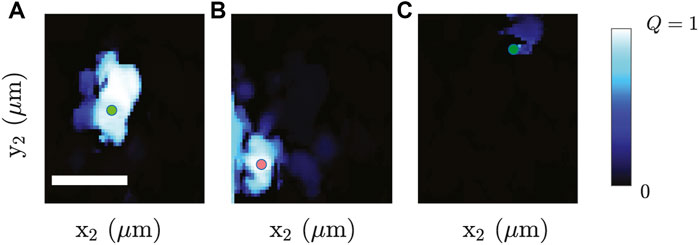
FIGURE 7. Q-maps. Panels (A–C) show Q-maps for modes (a), (e), and (c), respectively. Data are from [35].

A similar situation is found in Figure 7B for the mode in e_i. The two modes are only barely overlapping: energy is not flowing from one localized state to the other. The dark area in both maps corresponds to locations in which no intensity is transferred to the localized state. Note that the small displacements of the input inside the dwelling area do not cause any modification in the mode fingerprint. Multimode light structures would give rise to a pronounced flickering of the image due to the difference in phase delay of the different modes. The absence of such flickering is a relevant proof of the single-mode nature of the light structures supported by the DBFs.

The fact that the dwelling areas of different modes are barely overlapping is consistent with the picture in which localized states are orthonormal. A definitive confirmation of orthonormality requires to measure all the relevant observables: dwelling area, fingerprint, spectral parameter, and polarization. Such a challenging experiment (requiring the full characterization of thousands of modes) has not yet been carried on to our knowledge.

On the other hand, Figure 7C, related to mode (c_i), provides a Q-map almost entirely empty: in absence of a transmission channel, retrieved light is not coupled to a localized state. In this case the fiber behaves in way similar to a (very leaky) large-core multimode fiber where a small translation of the input produces a complete change of the output due to interference (thus an immediate decay of the Q value).

Regarding polarization, [24] reports one of the first studies about the impact of polarization: in the Supplementary Figure S3 of reference [24], the authors show that image reconstruction is nearly unaffected by the input polarization. The Supplementary Figure S2 of reference [35] demonstrates the “polarization maintaining” nature of the localized states. To our knowledge, there are no experimental studies for the polarization behavior in the nonlinear case; however, we have no evidence suggesting that the picture changes.

The summary is as follows

1) High transmission channels in a fiber are sparse.

2) They are separated by a barely transmitting “sea”.

3) Independently on how (and where) light is coupled to a fiber, each transmission channel retains its fingerprint (output profile).

4) Modes are excited in alternative fashion (i.e., the same input location activates only a transmission channel at time).

In other words, localized states of a disordered binary fiber behave exactly like the single modes of conventional single mode fibers showing the same property: namely the “resilience to the launch conditions.”

2.7 Designed Disorder in Glass Fibers

Disorder binary fibers (DBF) are a unique architecture [36]: a fiber without cores (thus similar to a multimode fiber), capable of hosting localized/single mode solutions. However, the high absorbance of the plastic component materials, together with fabrication-induced scattering losses, degrades consistently their transmittance efficiency, which remains very limited especially if compared with the properties of silica fibers capable to transmit light for kilometer with few losses. It is thus very promising to obtain transverse localization on disordered glassy fibers. The first observation of transverse Anderson localization in a glass optical fiber has been obtained by Mafi and coworkers [37]. The glassy disordered fiber has been obtained, starting from a “porous satin quartz” rod of 8 mm in diameter and 850 mm in length from which a single 150 m long fiber (diameter 250 µm) has been obtained. However, in this system the nonhomogeneous distribution of disorder (lower air hole density in the central region of the fiber) produces localized states only at the borders of the fiber. This uneven distribution of disorder forbids a complete optical exploitation of the waveguide section. Moreover, the positions of the defects (the air bubbles) are random (it results from the natural occurrence of pores in the rod) and cannot be tuned by the experimentalist at the fabrication stage.

On the other hand, the concept of designed disorder [38] is becoming an intense field of research with applications ranging from the fabrication of waveguides polarizering to light harvesting [39–41]. In fact, in some cases, disordered structures, even if fully deterministic, can be more favorable for specific tasks than periodic ones. For example, disordered arrays of defects can be employed to produce a structure displaying different propagation regimes (full photonic bandgap, Anderson localization, or free diffusion), depending on the wavelength employed [42].

In order to implant “designed disorder” into glassy optical fibers, the authors of [43] employed the femtosecond direct laser writing (FDLW) technique. FDLW [44] exists since the early nineties and enables nanometric resolution in surface ablation. In transparent materials bulk micro machining can be achieved through nonlinear (two- or three-photon) absorption, thus enabling the fabrication of photonic or microfluidic devices. The strong confinement of the nonlinear absorption volume, together with positioning performed by piezo-actuators with nanometric resolution, enables the fabrication of three-dimensional and complex structures. The modifications by nonlinear absorption yield a local refractive-index change (at low power) or even void formation (at high power). Importantly the changes produced are permanent; thus, the low power approach enables producing durable wave guides. The group of Szameit and coworkers reported several experiments on waveguide arrays in which disorder is introduced in the inter-waveguide coupling factors. This approach enabled to investigate Anderson localization [45–48], defect localization [49], and also topological insulation [50]. This wave-guide-based approach, indeed, enables accessing a plethora of intriguing physical phenomena; however, it requires the individual fabrication of each of the transmission channels. In this sense, DBF support localization in a different manner: they can be, indeed, seen as a continuous meta-material, potentially hosting localized states at any location, which could support the resonance condition. The most evident consequence of this difference is that localized states translate gradually their position when wavelength is changed in DBF, while they can be hosted only at the waveguides location in waveguides-arrays.

In order to transfer the advantage of DBF to glasses, Gianfrate and coworkers [43] employed FDLW in a nontraditional way. In particular they employed an objective with high numerical aperture (NA = 0.65) to generate tubes with very small diameter and with refractive index larger than the surrounding medium. These paraxial structures play the role of a transverse scatterer, because their reduced transverse dimension does not enable to support propagating modes: they act as paraxial defects (see sketch in Figure 1). This new generation of optical fibers based on paraxial defects has been studied in [43], where the authors show how the localization strength depends on the degree disorder properties. The authors demonstrate that the confinement properties depend on the degree of disorder 0 < χ < 1: a parameter tuned at the fabrication stage. The paraxial defects are fabricated at the transverse coordinates $[X_{M_x},Y_{M_y}]=[\delta (M_x+\chi {\theta }_{M_x}),\delta (M_y+\chi {\theta }_{M_y})]$, where M_x and M_y are integer numbers between 0 and S and δ is the lattice size and θ is a uniform random number between [−0.5 and 0.5]. When χ is 0, the paraxial defects are located in a square lattice with cell side δ and S² defects (square with side δS). For χ > 0 each defect is displaced by a random amount δχθ_Mx along X and δχθ_My along y, generating a square lattice with an increased degree of randomness.

Figure 8 reports the measured localization length ξ as a function of χ. It is possible to note that the localization length decreases up to 0.6 and then starts to increase again. While the decrease is naturally expected as a natural consequence of increasing disorder, the increasing behavior above χ = 0.6 results from the appearance of overlapping paraxial defects which are effectively decreasing the defect density.

FIGURE 8

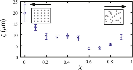
FIGURE 8. Localization length in direct laser written disorder. Localization length ξ versus degree of disorder χ, measured in a D Glassy substrate in which paraxial defects have been realized with FDLW. Data are from [43].

The realization of localization induced by direct laser-written defects is the first step towards a new generation of glass-based optical fibers characterized by low absorption and greater stability with respect to their plastic counterpart. The ability of tuning the defect position will open the possibility to test the concepts of designed disorder directly in optical fibers, thus paving the way towards unprecedented applications.

3 Theory of Anderson Localization of Light

3.1 Historical Overview

Since the appearance of Anderson’s seminal 1958 article [17], the interest of the condensed-matter community in electron and wave localization has not decreased [31, 51]. That Anderson localization is an interference phenomenon, i.e., due to the wave nature of electrons, became only clear in a second seminal paper by the “gang of four” Abrahams, Anderson, Licciardello and Ramakrishnan [20], in which they combined perturbation theory with a scaling procedure (to be described below) to show that the disorder-induced interference leads always to localization in two and one dimension. That one-dimensional systems feature always localized states had already been shown by Mott and Twose in 1961 [52].

The rather ad-hoc scaling argument of the gang of four has been given two complementary field-theoretic fundaments: the self-consistent localization theory of Vollhardt and Wölfle [53–55] and the generalized nonlinear sigma model [56, 57], which goes back to a paper by Wegner [58]. Wegner realized that the nonlinear sigma model for planar ferromagnetism exhibits the same scaling behavior as the scaling theory of Anderson localization. Shortly after the self-consistent localization theory of Vollhardt and Wölfle [53–55] appeared, it was noted by Economou and Soukulis [59] that the resulting self-consistent equation for finding the localization length was mathematically analogous to the problem of finding (or not finding) a bound state for single electrons within a potential well (“potential-well analogy”). The potential-well-analogy method was later formulated more rigorously by Soukoulis et al. [60] and Zdetsis et al. [61]. In all three analytic approaches, 1) the scaling/nonlinear sigma model theory, 2) the self-consistent theory, and 3) the potential-well analogy, one proceeds in two steps for calculating the localization characteristics, namely the phase diagram, the conductance in the delocalized regime, and the localization length in the localized regime:

1) Calculating a “unrenormalized” (or “reference”) conductance g₀ from the disorder statistics of the spatially fluctuating potential

2) Applying the

- scaling equations (scaling theory/nonlinear sigma model)

- self-consistency relation (self-consistent localization theory)

- potential-well relation.

It is interesting to note that as the potential-well analogy is not based on the assumption of weak disorder (i.e., the assumption that the relative variance of the potential fluctuations is small), one can apply the standard effective-medium theory for strong disorder, namely the coherent-potential approximation (CPA) for calculating g₀ [61]. Complementary numerical methods for solving the Anderson localization problem are the Green’s function method [62, 63] and the transfer matrix method [64]. In both methods the one-parameter scaling idea is used to extract the bulk localization features by finite-size scaling. These methods do not suffer from some shortcomings of the analytical approaches (The analytic approaches predict, e.g., a critical exponent of ν = 1.0, whereas the true one, obtained by the numerical work, is ν = 1.57 [62, 65]).

The standard (Anderson) model for electron localization is given by the following Hamiltonian on a simple hypercubic lattice [17] with lattice constant a.

$\mathcal{H}=\sum _i|i>{ϵ}_i<i|+t\sum _{i\ne j}|i><j|(10)$

where the indices i, j denote lattice sites and the double sum is over next nearest neighbors only. ϵ_i = < i|V(r)|i > is the diagonal element of an external potential V(r), which varies randomly in space. < r|i > are Wannier basis states. Usually the local potentials ϵ_i are assumed to be independent random variables, which are distributed according to a distribution density P(ϵ), which can be a Gaussion or a box-shaped function [66]. The overlap (“hopping”) matrix element t is assumed to be constant. Near the bottom (or top) of the band, one can write down a continuum Hamiltonian,

$\mathcal{H}=-\frac{{\hslash }^2}{2m}{\nabla }^2+V(\mathbf{r})(11)$

with $t{a}^2=\frac{1}{2m}$. Here a constant 6t has been added (subtracted) at the bottom (top) of the band. This leads to the Schrödinger equation:

$E\psi (\mathbf{r})=\mathcal{H}\psi (\mathbf{r})=\left(-\frac{{\hslash }^2}{2m}{\nabla }^2+V(\mathbf{r})\right)\psi (\mathbf{r})(12)$

In the continuum description [57], one considers V(r) as a Gaussian random variable with zero mean and correlation function < V(r)V (r′) > = γδ(r −r′), where γ is the variance times a d-dimensional volume.

As there is no difference from the mathematical standpoint between a time-Fourier transformed classical wave equation (Helmholtz equation) and the Schrödinger Eq. 12 for the electrons (identifying 2mE/ℏ² with −ω², where ω is the angular frequency), it was soon suggested that acoustical [67] and electromagnetic (EM) waves [68, 69] should also exhibit Anderson localization. These theoretical approaches were based on the nonlinear-sigma-model formalism. A multiple-scattering approach for localization of (schematically scalar) acoustical waves was published by Kirkpatrick (1985) [70].

Considering acoustical waves in a disordered medium, the disorder may come from 1) spatial density fluctuations or 2) spatial fluctuations of elastic moduli. John et al. [67] assumed density fluctuations, and the approach of Kirkpatrick (see Eqs 6a–6c of [70]) is equivalent to considering fluctuating elastic moduli. If one assumes both density and modulus fluctuations, the wave equation for the schematically scalar acoustical displacement field ϕ(r, t) takes the form

$\rho (\mathbf{r})\frac{{\partial }^2}{\partial t^2}\varphi (\mathbf{r},t)=\nabla K(\mathbf{r})\nabla \varphi (\mathbf{r},t)(13)$

or in frequency space

$-\rho (\mathbf{r}){\omega }^2\varphi (\mathbf{r},t)=\nabla K(\mathbf{r})\nabla \varphi (\mathbf{r},t)(14)$

If the density ρ does not fluctuate, Eq. 14 constitutes an ordinary eigenvalue problem, which can be solved by discretization, followed by diagonalization. In the case of density fluctuations, one can separate the fluctuations from the mean ρ(r) = ρ₀ + Δρ(r):

$-{\rho }_0{\omega }^2\varphi (\mathbf{r},t)=\left({\omega }^2\mathrm{\Delta }\rho (\mathbf{r})+K{\nabla }^2\right)\varphi (\mathbf{r},t)(15)$

Now the term ω²Δρ(r) looks like a frequency-dependent potential. But from the mathematical standpoint, it is strange that in an eigenvalue problem the potential depends on the eigenvalue. Certainly it would be more sound to divide the whole equation by ρ(r) to obtain an effective modulus K(r)/ρ(r). However, in their approach to acoustical localization, John et al. [67] kept the effective frequency-dependent potential, because then they could take over the established electronic theory of Anderson localization, in particular the nonlinear-sigma-model theory of McKane and Stone [57]. In his seminal article on the localization of light [71], the author pursued the same strategy: he wrote down a wave equation for the electrical field E(r, ω), where the ω² term was multiplied with the spatially varying permittivity ϵ(r). In this derivation, he tacitly assumed that the divergence of E would be zero. We pointed already out that, in the presence of a disorder-induced spatially varying permittivity, this is not the case. We shall discuss the consequences of this in the sections after introducing the scaling concept of localization theory.

For later reference, let us call a stochastic wave equation with fluctuating coefficient of ω² a “potential-type” (PT) equation and, if the elastic modulus fluctuates, a “modulus-type” (MT) stochastic equation.

Pinski et al. [65, 69] used the transfer matrix method to solve the discretized stochastic acoustic wave Eq. 14 for the density of states and the localization properties, comparing the MT case with the PT case. While they find that the critical properties of both models are within the universality class of the electronic Anderson problem [72], the phase diagrams of the two models are rather different. The analogue of the PT model is the Anderson model of Eqs. 10, 12, whereas the quantum analog of the MT model is an electron system with spatially fluctuating hopping amplitude or effective mass (“off-diagonal disorder”) [73], which also has a phase diagram different from the Anderson model [73]. So one can state that the PT and MT stochastic wave equations describe two physically different situations of wave disorder. In the case of electromagnetic case, however, they are supposed to describe the same, namely EM waves in a medium with spatially fluctuating permittivity ϵ(r) = n²(r). The solution of this paradox is, as we shall demonstrate below, that the PT description is an approximation (neglecting the ∇ E term), whereas the MT description is exact.

3.2 Wave Interference and the Scaling Theory of Anderson Localization

If a wave is experiencing disorder like electrons in an impure metal, the waves are repeatedly scattered. This multiple scattering process can be interpreted as a random walk, featuring a diffusion constant D. In fact, one can derive a diffusion equation for the wave (diffusion approximation [74, 75]). The diffusion approximation is equivalent with the relaxation time approximation [76], leading to the Drude law for the conductivity.

The diffusion approximation assumes that after each scattering event, the phase memory is lost. However, if one follows the scattering amplitudes with phases kł_ij (where l_ij is the distance between two adjacent scattering centers) in a frozen medium, the phase memory is in principle not lost. This has dramatic consequences for recurrent partial paths, i.e., paths with closed loops: the phase of the recurrent path is exactly equal to that going in the reverse direction (see Figure 9). This leads to destructive interference and therefore to a decrease of the diffusivity and, as we shall see, for d = 2 to a vanishing of the diffusivity.

FIGURE 9

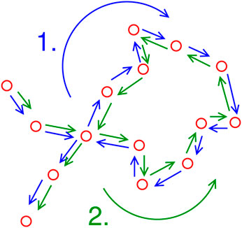
FIGURE 9. Visualization of two interfering scattering parts, one going clockwise along the loop and the other anticlockwise.

For describing the interference mechanism, Abrahams et al. [20] have proposed an ingenious scaling scenario. They consider the dependence of a dimensionless conductance g on the sample size L in d dimensions and make the Ansatz

$g(L)\propto L^{\beta }\iff \beta =\frac{d\ln g}{d\ln L}(16)$

For β > 0 g scales towards infinity with increasing L, β < 0 g scales towards zero. In the metallic regime (g → ∞), the conductance should depend on the size L of a sample as g(L) ∝ σL^d−2, where σ is the conductivity, so that β(g → ∞) = d − 2 (see Figure 10). On the other hand, for localization (g → 0) one expects g(L) ∝ e^−L/ξ, where ξ is the localization length. This transforms to β(g → 0) ∝  ln g. Abrahams et al. then assumed a smooth interpolation between the two limits to exist (see Figure 10). By means of perturbation theory, they further estimated the correction due to the interference terms to be negative and proportional to 1/g. Their final result for the scaling function is

$\beta (g)=\frac{\partial \ln g}{\partial \ln L}=d-2-\frac{c}{g}(17)$

where c is a dimensionless constant of the order of 1. It can be verified from Figure 10 that in 3 dimension, the scaling with increasing size L depends on the initial value of the conductance, i.e., on the conductivity in diffusion approximation (Drude approximation for electrons). However, as can be seen from Figure 10 in 2 and 1 dimension, g scales always towards 0, i.e., for L → ∞, there is always localization.

FIGURE 10

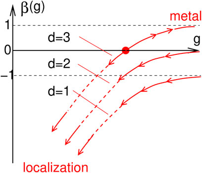
FIGURE 10. Sketch of the scaling function as anticipated by Abrahams, Anderson, Licciardello, and Ramakrishnan [20].

The scaling function (Eq. 17) is the same for the nonlinear sigma model for planar ferromagnetism, as noticed by Wegner [58]. Later a field-theoretical mapping from a stochastic Helmholtz equation to a generalized nonlinear sigma model was established and applied to the electronic Anderson problem [56, 57] as well as the PT description of the classical-wave problem [1, 67] and the MT description of acoustical [77] waves and light [26].

In two dimensions, the scaling Eq. 17 is solved as

$g(L)=-c\ln L/L_0+g_0(18)$

The localization length is given by the value L taken for g₁ ≈ 1. The reference conductance g₀ is the diffusion-approximation conductance

$g_0=k\ell ,(19)$

where k is the wave number and ℓ the mean free path. For the reference length, traditionally the mean-free path has been taken as well. In our description, instead, we shall take for L₀ the correlation length L_c of the disorder fluctuations (see below)

$L_0=\frac{1}{q_c}=\frac{L_c}{2\pi }(20)$

From Eq. 18 one obtains the well-known formula [78] for two dimensions:

$\xi (E)=\frac{1}{q_c}{e}^{g_0(\mathsf{E})/c}(21)$

3.3 Wave Equation for Electromagnetic Waves in a Disordered Environment

As indicated above, almost the entire literature on Anderson localization (AL) of light is based on the potential-type wave equation, i.e., a wave equation in which the spatially fluctuating permittivity ϵ(r) appears as a coefficient of the double-time derivative of the wave function (electric field). In a recent article [26], some of the present authors have shown that this wave equation is in error and leads to a fictitious wavelength dependence of the localization length in transverse localization, which is not observed in the experiments. We now review the derivation of the traditional wave equation, showing which error was made, and present the derivation of the correct wave equation.

Maxwell’s equations in a medium with spatially varying permittivity ϵ(r) are

$\begin{array}{lll}\hfill \nabla \cdot \mathbf{B}(\mathbf{r},t)=0& \hfill & \hfill \nabla \cdot \mathbf{D}(\mathbf{r},t)=0\mathbf{D}(\mathbf{r},t)=ϵ(\mathbf{r})\mathbf{E}(\mathbf{r},t)\end{array}(\mathrm{22a})$

$\begin{array}{lll}\hfill & \hfill & \hfill \\ \hfill \nabla \times \mathbf{B}(\mathbf{r},t)& =\frac{1}{c^2}\frac{\partial }{\partial t}\mathbf{D}(\mathbf{r},t)\nabla \times \mathbf{E}(\mathbf{r},t)=-\frac{\partial }{\partial t}\mathbf{B}(\mathbf{r},t)\hfill & \hfill \end{array}(\mathrm{22b})$

For deriving a wave equation for the electromagnetic fields, one can either solve the electrical field E(r, t) or the magnetic field B(r, t).

3.3.1 Traditional, Potential-Type Approach

The traditional procedure (potential-type approach, PT) was to solve E(r, t):

$\begin{array}{ccc}\hfill \frac{ϵ(\mathbf{r})}{c_0^2}\frac{{\partial }^2}{\partial t^2}\mathbf{E}(\mathbf{r},t)& =\hfill & -\nabla \times \nabla \times \mathbf{E}(\mathbf{r},t)\hfill \\ \hfill & =\hfill & {\nabla }^2\mathbf{E}-\nabla \left(\nabla \cdot \mathbf{E}(\mathbf{r},t)\right)\hfill \\ \hfill & \approx \hfill & {\nabla }^2\mathbf{E},\hfill \end{array}(23)$

where in the last step ∇ ⋅E = 0 was assumed. In the frequency regime, we obtain the following stochastic Helmholtz equation:

$-{\omega }^2\frac{ϵ(\mathbf{r})}{c_0^2}\mathbf{E}(\mathbf{r},\omega )\approx {\nabla }^2\mathbf{E},(24)$

which, separating the fluctuations of the permittivity as ϵ(r) = <ϵ> + Δϵ(r), can be rewritten as

$-{\omega }^2\frac{⟨ϵ⟩}{c_0^2}\mathbf{E}(\mathbf{r},\omega )\approx \left({\nabla }^2+\underset{\mathcal{V}(\omega )}{\underbrace{{\omega }^2\frac{\mathrm{\Delta }ϵ(\mathbf{r})}{c_0^2}}}\right)\mathbf{E}(25)$

This equation is mathematically equivalent to a stationary Schrödinger equation for an electron in a frequency-dependent random potential $\mathcal{V}(\omega )$. This equivalence made it possible to transfer the complete electronic theory of AL [21, 53] to classical electromagnetic waves [21, 71, 79, 80]. We call this approach “potential-type” (PT).

We now want to check the validity of the approximation made in Eqs 23–25. We have

$0=\nabla \cdot \mathcal{D}=\nabla \cdot \left(ϵ(\mathbf{r})\mathbf{E}(\mathbf{r})\right)=ϵ(\mathbf{r})\nabla \cdot \mathbf{E}(\mathbf{r})+\mathbf{E}(\mathbf{r})\cdot \nabla ϵ(\mathbf{r})(26)$

from which follows [81].

$\nabla \cdot \mathbf{E}=-\frac{1}{ϵ(\mathbf{r})}\mathbf{E}\cdot \nabla ϵ(\mathbf{r})\ne 0(27)$

One can estimate the error made in Eq. 23 by inserting for E a wave with wavelength λ. If the scale, on which the permittivity is varying, is large with respect to λ (eikonal limit), the term on the right-hand side of Eq. 27 is negligible. However, if this condition is fulfilled, one deals with very weak disorder. In this case, one has in three-dimension delocalization and in two dimension a very large localization length, exceeding macroscopic sample dimensions, which would make the observation of AL impossible. So, for stronger disorder, where one might have a chance for observing AL, the scale of the permittivity fluctuations must be of order λ. In this case the divergence of E is not negligible. This renders the approximation made in the PT wave Eq. 23 invalid.

3.3.2 New Approach: Modulus-Type Description

If one solves the Maxwell Eq. 22 for B, one obtains

$\frac{{\partial }^2}{\partial t^2}\mathbf{B}(\mathbf{r},t)=-\nabla \times \frac{c_0^2}{ϵ(\mathbf{r})}\nabla \times \mathbf{B}(\mathbf{r},t)(28)$

Equation 28 leads to the following stochastic Helmholtz equation:

${\omega }^2\mathbf{B}(\mathbf{r},\omega )=\nabla \times M(\mathbf{r})\nabla \times \mathbf{B}(\mathbf{r},\omega ),(29)$

where we have defined the spatially fluctuating dielectric modulus as $M(\mathbf{r})=c_0^2/ϵ(\mathbf{r})$.

Equation 29 is mathematically equivalent to the Helmholtz equation for an elastic medium with zero bulk modulus and a spatially fluctuating shear modulus M(r). This equation is exact and is called the modulus-type (MT) approach. A theory for a medium with finite (constant) bulk modulus K and a spatially fluctuating shear modulus has been worked out [77, 82, 83] by some of the present authors and applied for explaining the anomalous vibrational properties of glasses, in particular the enhancement of the vibrational density of states with respect to the Debye law (“boson peak”). Our present theory of Anderson localization of light relies on the analogy to this case. Essentially one needs only to take the K → 0 limit for this theory and obtain a theory for light diffusion and localization in disordered optical systems.

In order to describe transverse Anderson localization, we first map this problem to a two-dimensional problem. We then use the paraxial approximation to map the z dependence of the wave profiles to the time dependence in an effective Schrödinger equation. For estimating the diameter of the large-z profile, the localization length ξ, we apply the scaling theory of Anderson localization [20, 21], which is equivalent to the renormalization-group approach to the generalized nonlinear sigma model [56–58]. For the calculation of the z dependence of the localization length, we then use the self-consistent localization theory of Vollhardt and Wölfle [53–55, 80].

3.4 Description of Optical Fibers With Transverse Disorder

We now consider an optical fiber with transverse disorder, i.e., the permittivity exhibits spatial fluctuations in x and y direction, but not in z direction.

Because our system is translation invariant with respect to the z direction, we may take a Fourier transform with respect to z: $\mathbf{B}(x,y,k_z,\omega )=\int dz{e}^{i{k}_{z}z}\mathbf{B}(x,y,z,\omega )$. We then obtain an effective two-dimensional Helmholtz equation

$(\underset{\mathsf{E}=k_{\perp }^2}{\underbrace{[k_0^2-k_z^2]}}-{\nabla }_{\perp }\times \frac{M(x,y)}{⟨M⟩}\times {\nabla }_{\perp })\mathbf{B}(x,y,k_z,\mathsf{E})=0(30)$

where $k_0=\omega /\sqrt{⟨M⟩}=2\pi /\lambda$ is the wavenumber of the input laser beam, λ is its wavelength, and θ is the angle between the direction of the incident beam direction and the optical axis (azimuthal angle); see Figure 1. $\mathsf{E}=k_{\perp }^2=k_0^2-k_z^2=k_0^2{\sin }^2\theta$ is called the spectral parameter. It replaces the spectral parameter ω² of a true two-dimensional system.

For θ ≪ 1 we can make the approximation E = (k₀ + k_z) (k₀ − k_z) ≈ − 2k₀ (k_z − k₀) ≡ −2k₀Δk_z, which is called the paraxial approximation [16]. The wavenumber Δk_z refers to the Fourier component of the envelope$\mathit{b}(x,y,z)=\mathbf{B}(x,y,z)e^{-i{k}_{0}z}$, which describes the beats of the magnetic field vector B(x, y, z) in z direction. In the paraxial limit b(x, y, z) obeys the paraxial equation

$\left(2i{k}_0\frac{\partial }{\partial z}+{\nabla }_{\perp }\times \frac{M(x,y)}{⟨M⟩}\times {\nabla }_{\perp }\right)\mathit{b}(x,y,z)=0.(31)$

Introducing a “time” τ = z/2k₀ (which has the dimension of a squared length), this equation acquires the form of a Schrödinger equation of an electron in a medium with a randomly varying effective mass:

$\left(\frac{\partial }{\partial \tau }+{\nabla }_{\perp }\times \frac{M(x,y)}{⟨M⟩}\times {\nabla }_{\perp }\right)\mathit{b}(x,y,\tau )=0.(32)$

As stated above, such a model is related with a stochastic tight-binding model with a spatially varying hopping amplitude (“off-diagonal disorder”) [73].

Let us now compare the MT Eq. 31 with Eq. 5,

$(2i{k}_0\frac{\partial a(\mathbf{r})}{\partial z}-{\nabla }_{\perp }^2-\underset{U(x,y)}{\underbrace{k_0^2\left[\frac{n{(x,y)}^2-n_0^2}{n_0^2}\right]}})a(x,y)\left.\right)=0$

By comparing Eq. 31 with Eq. 5, we can estimate the influence of the wavelength λ = 2π/k₀ on the localization properties: in the exact MT Eq. 31 the wavenumber k₀ enters only as a prefactor of the z derivative. Therefore, in the steady-state regime z → ∞ k₀ does not enter at all. This is, however, completely different for the PT case described by Eq. 5: here k₀ is the prefactor of the fluctuating-disorder term, which governs the mean-free path and hence the localization length.

How come that the predictions of two wave equations which are supposed to describe the same physical situation, namely, the wave propagation (or localization) of samples with transverse disorder, differ in such a drastic way? The difference can be traced back to the fact that in deriving (Eq. 5) the term ∇ ⋅E has been dropped. Therefore, the additional wavelength dependence implied by the PT Eq. 5 must be an artifact of this approximation. We shall come back to the comparison between the PT and MT predictions when we display explicit results obtained in the two approaches.

3.5 Mean-Field Theory for Wave Propagation in a Turbid Medium

3.5.1 Rayleigh Scattering and Disorder

The most important aspect of Anderson localization is the disordered environment. In the case of electromagnetic wave, the disorder may appear as randomly distributed scatterers or a spatially fluctuating permittivity ϵ(r) = n²(r).

Lord Rayleigh considered in his seminal papers on the blue color of the sky [84, 85] point-like scatterers, which act like induced Hertzian dipoles. Jackson points out in his textbook [86] that considering fluctuating permittivity one obtains as well the famous ω⁴ law for the scattering cross-section, which is inversely proportional to the mean-free path. It is known nowadays that this law becomes ω^d+1 in d dimensions [87, 88].

Because in our effective two-dimensional system the wave spectral parameter ω² is replaced by $\mathsf{E}=k_{\perp }^2$ for small E, we must have by the two-dimensional Rayleigh law

$\frac{1}{\ell (\mathsf{E})}\propto k_{\perp }^3={\mathsf{E}}^{3/2}(33)$

We shall demonstrate in Section 3.7 that the PT approach violates this requirement.

For weak disorder¹, i.e., $\langle \mathrm{\Delta }M{\left.\right)}^2\rangle \ll \langle {M\rangle }^2$, the detailed distribution of the moduli (Gaussian or otherwise) is not important, because—as we shall see—the only parameters which enter into the mean-free path are the mean 〈M〉, the variance 〈ΔM²〉, and the correlation length L_c of the fluctuating inverse permittivity (modulus). Here ΔM(ρ) = M(ρ) −〈M〉 are the fluctuations about the mean. Here and in the following ρ signifies the two-dimensional spatial vector.

The correlation length of the spatially fluctuating modulus is an important parameter, because it defines the characteristic length scale of these fluctuations. It is defined by the length scale of the spatial decay of their correlations:

$L_c^2=\frac{1}{⟨\mathrm{\Delta }{M}^2⟩}\int d^2\mathit{\rho }C(\mathit{\rho })(34)$

with the correlation function

$C(\mathit{\rho })=⟨\mathrm{\Delta }M(\mathit{\rho }+{\mathit{\rho }}_0)\mathrm{\Delta }M({\mathit{\rho }}_0)⟩(35)$

3.5.2 Simplified Scalar MT Model and Born Approximation

In this introductory subsection, we consider a simplified MT Helmholtz equation for a schematic scalar wave function $b(\mathit{\rho },E)$

$\mathsf{E}+{\nabla }_{\perp }\cdot \left(1-\frac{\mathrm{\Delta }M(\mathit{\rho })}{⟨M⟩}\right)\cdot {\nabla }_{\perp }\left.\right)b(\mathit{\rho },\mathsf{E})=0(36)$

The corresponding Green’s function obeys

$\left[s+{\nabla }_{\perp }\cdot \left(1-\frac{\mathrm{\Delta }M(\mathit{\rho })}{⟨M⟩}\right)\cdot {\nabla }_{\perp }\right)\mathsf{G}(\mathit{\rho },{\mathit{\rho }}^{\prime },s)=-\delta (\mathit{\rho }-{\mathit{\rho }}^{\prime }),(37)$

where s = E + iϵ is the complex spectral parameter.

It has been shown in [89] that for sufficient small spectral parameter one can use the Born Approximation with respect to the fluctuations ΔM of the (in this case elastic) modulus. In order to apply the Born approximation, the Fourier-transformed averaged Green’s function is represented in terms of a complex self-energy function Σ(E):

$\begin{array}{ccc}\hfill G(q,s)& =\hfill & \int d^2\{\mathit{\rho }-{\mathit{\rho }}^{\prime }\}{e}^{i\mathbf{q}[\mathit{\rho }-{\mathit{\rho }}^{\prime }]}⟨\mathsf{G}(\mathit{\rho },{\mathit{\rho }}^{\prime },\mathsf{s})⟩\hfill \\ \hfill & =\hfill & \frac{1}{-s+q^2\left[1-\mathrm{\Sigma }(s)\right]}\hfill \end{array}(38)$

and the lowest quadratical order in ΔM is given by

$\mathrm{\Sigma }(s)=\frac{1}{{(2\pi )}^2}\frac{1}{{⟨M⟩}^2}\int d^2\mathbf{q}{q}^{2}C(\mathbf{q})G_0(q,s)(39)$

with the unperturbed Green’s function

$G_0(q,s)=\frac{1}{-s+q^2}.(40)$

We now represent the correlation function schematically by introducing an upper wavenumber cutoff $q_c\propto L_c^{-1}$:

$C(q)=C_0\frac{1}{q_c^2}⟨{(\mathrm{\Delta }M)}^2⟩\theta (q_c-q),(41)$

where C₀ is a dimensionless constant and θ(x) is the Heaviside step function. From this we get, using the fact that the Green’s function does only depend on q = |q|,

$\mathrm{\Sigma }(s)=C_0\frac{1}{q_c^2}\frac{\langle {(\mathrm{\Delta }M)}^2\rangle }{\langle {M\rangle }^2}\frac{1}{2\pi }{\int }_0^{q_c}dq{q}^3{G}_0(q,s)(42)$

We fix C₀ by requiring that the q sum

$\sum _{\mathbf{q}}\equiv C_0\frac{1}{q_c^2}\frac{1}{2\pi }{\int }_0^{q_c}qdq\stackrel{!}{=}1,(43)$

i.e., C₀ = 4π. We finally get for the self-energy

$\mathrm{\Sigma }(s)=\gamma \sum _{\mathbf{q}}{q}^2{G}_0(q)(44)$

with the “disorder parameter” γ = 〈 (ΔM)² 〉 / 〈M 〉². The inverse mean-free path is given by the imaginary part of Σ, multiplied with k_⊥ (see the next subsection):

$\frac{1}{\ell (\mathsf{E})}=k_{\perp }{\mathrm{\Sigma }}^{″}(\mathsf{E})(45)$

The integral in Eq. 42 or Eq. 44 is elementary and gives $k_{\perp }^2\pi /q_c^2$ for k_⊥ ≤ q_c, so that we obtain from the Born approximation (Eq. 42) the Rayleigh law (Eq. 33)

$\frac{1}{\ell (\mathsf{E})}=\gamma \pi k_{\perp }^3/q_c^2{k}_{\perp }\le q_c,(46)$

which, as said above, holds in the limit $E=k_{\perp }^2\to 0$

3.5.3 Self-Consistent Born Approximation (SCBA) for the Modulus-Type Approach

For higher values of the spectral parameter, the Born approximation is insufficient, and we need a nonperturbative approach. Using a hand-waving argument, stating that it is inconsistent to work with two different Green’s functions, one may replace G₀ (q, s) in the Born approximation for Σ(s) by the full Green’s function G (q, s). This turns Eq. 44 into a nonlinear, self-consistent equation for Σ(s). This is the self-consistent Born approximation (SCBA):

$\mathrm{\Sigma }(s)=\gamma \sum _{\mathbf{q}}{q}^{2}G(q,s)=\gamma \sum _{\mathbf{q}}\frac{q^2}{-s+q^2[1-\mathrm{\Sigma }(s)]}(47)$

The SCBA may be obtained more rigorously by field-theoretical techniques [56, 57, 67, 77], in which it appears as a saddle-point of an effective field theory.

For our detailed calculations² we return to the full vector Helmholtz Eq. 30. We take advantage of the fact that the equation of motion for an elastic medium with spatially fluctuating shear modulus μ(r) is of the form

$\left[{\rho }_m{\omega }^2+\nabla \cdot \left(\lambda +2\mu (\mathbf{r})\right)\nabla \cdot -\nabla \times \mu (\mathbf{r})\nabla \times \right]\mathbf{u}(\mathbf{r},\omega )=0(48)$

where u is the displacement vector, ρ_m the mass density, and λ is the longitudinal Lamé modulus. If one discards the longitudinal term, one arrives at the MT Eq. 30. Therefore one can take over the entire theory [77] derived for the classical sound waves without the longitudinal excitations, working in two instead in three dimensions. Within this theory the influence of transverse disorder is accounted for by an effective-medium treatment (self-consistent Born approximation, SCBA), derived as saddle-point approximation within the nonlinear sigma model field theory [77]. In such a treatment the spatial fluctuations of $\widetilde{ϵ}$ are transformed into a dependence on the complex spectral parameter s = E + i0 according to

$\begin{array}{ccc}\hfill \mathsf{G}(k,s)\equiv ⟨G(\mathbf{k},s)⟩& =\hfill & \frac{1}{-s+k^2[1-\mathrm{\Sigma }(s)]}\hfill \\ \hfill & =\hfill & \frac{1}{1-\mathrm{\Sigma }(s)}\left(\frac{1}{-k_{\mathrm{\Sigma }}^2+k^2}\right)\hfill \end{array}(49)$

where G (k, s) is the Fourier and Laplace transform of one of the two configurationally averaged Greens functions of Eq. 30 (which are equal to each other), and we now represent the Green’s function in the following way:

$\begin{array}{ccc}\hfill G(q,s)& =\hfill & \int d\{\mathit{\rho }-{\mathit{\rho }}^{\prime }\}{e}^{i\mathbf{q}[\mathit{\rho }-{\mathit{\rho }}^{\prime }]}⟨\mathsf{G}(\mathit{\rho },{\mathit{\rho }}^{\prime },\mathsf{s})⟩\hfill \\ \hfill & =\hfill & \frac{1}{-s+q^2\left[1-\mathrm{\Sigma }(s)\right]}=\frac{1}{1-\mathrm{\Sigma }(s)}\frac{1}{q^2-k_{\mathrm{\Sigma }}^2(s)}\hfill \end{array}(50)$

$\begin{array}{ccc}\hfill & \approx \hfill & \frac{1}{1-{\mathrm{\Sigma }}^{\prime }(0)}\frac{1}{q^2-k_{\mathrm{\Sigma }}^2(s)}\hfill \end{array}(51)$

where we have introduced an E dependent complex wave number k_Σ(s) = k_Σ′(E) + ik″_Σ(E), which obeys

$k_{\mathrm{\Sigma }}^2(s)=\frac{s}{1-\mathrm{\Sigma }(s)}(52)$

The SCBA self-consistent equation for Σ(s) is

$\mathrm{\Sigma }(s)=\gamma \sum _{\mathbf{q}}{q}^{2}G(q,s)=\gamma \sum _{\mathbf{q}}\frac{q^2}{-s+q^2\left(1-\mathrm{\Sigma }(s)\right)}=\frac{\gamma }{1-\mathrm{\Sigma }(s)}\left(1+sG(s)\right)(53)$

with the local Green’s function

$G(s)=\sum _{\mathbf{q}}G(q,s)=\frac{1}{1-{\mathrm{\Sigma }}^{\prime }}\sum _{\mathbf{q}}\frac{1}{-k_{\mathrm{\Sigma }}{(s)}^2+q^2}=\frac{1}{1-{\mathrm{\Sigma }}^{\prime }}\frac{1}{q_c^2}\left[\ln (q_c^2-k_{\mathrm{\Sigma }}^2)-\ln (-k_{\mathrm{\Sigma }}^2)\right].(54)$

From the local Green’s function, we obtain the spectral density as

$\rho (\mathsf{E})=\text{Im}\left\{\frac{1}{\pi }G(s)\right\}=\frac{1}{\pi }\sum _{\mathbf{q}}{G}^{″}(q,\mathsf{E})=\frac{1}{q_c^2(1-{\mathrm{\Sigma }}^{\prime })}\theta (q_c^2(1-{\mathrm{\Sigma }}^{\prime })-\mathsf{E})(55)$

For $\mathsf{E}\ll q_c^2$, we have

${\mathrm{\Sigma }}^{\prime }(\mathsf{E})\approx {\mathrm{\Sigma }}^{\prime }(0)=\frac{\gamma }{1-{\mathrm{\Sigma }}^{\prime }(0)}(56)$

which can be solved to give

$\mathrm{\Sigma }(0)=\frac{1}{2}\left(1-\sqrt{1-4\gamma }\right)\stackrel{\gamma \ll 1}{\approx }\gamma (57)$

Making a variable change v = q² and neglecting the imaginary part of $k_{\mathrm{\Sigma }}^2$ in the denominator, we obtain for the imaginary part of the self-energy

$\text{Im}\left\{\mathrm{\Sigma }(s)\left[1-\mathrm{\Sigma }(s)\right]\right\}={\mathrm{\Sigma }}^{″}(\mathsf{E})\left[1-2{\mathrm{\Sigma }}^{\prime }(\mathsf{E})\right]=\gamma \text{Im}\left\{\frac{1}{q_c^2}\int dv\frac{v}{-k_{\mathrm{\Sigma }}^{\prime 2}+v}\right\}=\gamma \frac{\pi }{q_c^2}{k_{\sigma }^{\prime }}^2(\mathsf{E}),(58)$

from which follows

${\mathrm{\Sigma }}^{″}(\mathsf{E})=\gamma \mathsf{E}\frac{\pi }{q_c^2}\frac{1}{1-2{\mathrm{\Sigma }}^{\prime }(\mathsf{E})}\frac{1}{1-{\mathrm{\Sigma }}^{\prime }(\mathsf{E})}\stackrel{\gamma \ll 1}{\approx }\gamma \mathsf{E}\frac{\pi }{q_c^2}(59)$

We now want to relate Σ″(E) to the mean-free path of the scattered waves. We may Fourier-transform the Green’s function (Eq. 37) into ρ space to obtain

$G(\mathit{\rho },s)=-\frac{1}{4(1-{\mathrm{\Sigma }}^{\prime })}{H}_0^{(1)}\left(k_{\mathrm{\Sigma }}(s)\rho \right)\stackrel{\rho \gg k_{\mathrm{\Sigma }}^{-1}}{\to }-\frac{1}{4\left(\right.1-{\mathrm{\Sigma }}^{\prime }}\sqrt{\frac{2}{\pi k_{\mathrm{\Sigma }}(s)\rho }}{e}^{i{k}_{\mathrm{\Sigma }}(s)\rho }(60)$

where $H_0^{(1)}(z)$ is the Hankel function of first kind [90]. For large ρ the intensity is then given by

${\left|G(\mathit{\rho },s)\right|}^2=\frac{1}{8\pi k_{\mathrm{\Sigma }}(s)\rho }{e}^{-\rho /\ell (\mathsf{E})}(61)$

with the mean-free path given by [26].

$\frac{1}{\ell (\mathsf{E})}=2k^{″}(\mathsf{E})=k_{\mathrm{\Sigma }}^{\prime }(\mathsf{E})\frac{{\mathrm{\Sigma }}^{″}(\mathsf{E})}{1-{\mathrm{\Sigma }}^{\prime }(\mathsf{E})}\propto {\mathsf{E}}^{3/2}(62)$

This generalizes the Born-approximation result (Eq. 46), which is reobtained for small E and/or small γ.

3.6 Self-Consistent Born Approximation for the PT Approach

The SCBA for the PT approach, due to John et al. [67], adapted to the transverse-disorder case reads [26]

${\mathrm{\Sigma }}_{PT}(s)=\gamma k_0^2\sum _{\mathbf{q}}{G}_{PT}(q,s)(63)$

with the Green’s function

$G_{PT}(q,s)=\frac{1}{-s-k_0^2{\mathrm{\Sigma }}_{PT}(s)+q^2}\equiv \frac{1}{-k_{\mathrm{\Sigma },PT}{(s)}^2+q^2}(64)$

As in the MT case, we have for the mean-free path

$\frac{1}{\ell (\mathsf{E})}={2k}_{\mathrm{\Sigma },PT}^{″}(\mathsf{E}).(65)$

3.6.1 Diffusion of the Wave Intensity

As the vector character of the magnetic field enters into our mean-field treatment only by doubling the Green’s functions, we return to a scalar description of the field amplitude.

The multiple scattering of waves in a turbid medium can be well described in terms of a random walk along the possible paths among the scattering centers [74]. The scattered intensity may be shown to obey a diffusion equation. Our object of interest is therefore the intensity propagator

$\begin{array}{ccc}\hfill P(\mathbf{q},p,\mathsf{E})& =\hfill & \frac{1}{{(2\pi )}^2}\int d^2\mathbf{k}\langle G\left(\mathbf{k}+\frac{1}{2}\mathbf{q},s_{+}+\frac{1}{2}\omega \right)G\left(\mathbf{k}-\frac{1}{2}\mathbf{q},s_{-}-\frac{1}{2}\omega \right)\rangle \hfill \\ \hfill & =\hfill & {\int }_{-\infty }^{\infty }d\mathit{\rho }{\int }_0^{\infty }d\tau e^{-p\tau }{e}^{-i\mathit{\rho }\mathbf{q}}P(\mathit{\rho },\tau ,\mathsf{E})\hfill \end{array}(66)$

with p ≡ −iω + ϵ, ϵ → + 0. The second line defines P (q, p, E) as the spatial Fourier transform and Laplace transform (with respect to τ) of the intensity propagator P (ρ, τ, E) in the ρ = (x, y) plane. For deriving the diffusion description, it is assumed that after each scattering event the memory of the phase of the wave function is lost. P (q, p, E) then obeys a diffusion equation with a E dependent modal “diffusivity”³D(p, E):

$\left(\frac{\partial }{\partial \tau }-{\nabla }_{\mathit{\rho }}^2{D}_0(\mathsf{E})\right)P(\mathit{\rho },\tau ,\mathsf{E})=\delta (\mathit{\rho })\delta (\tau )\iff P(\mathbf{q},p,\mathsf{E})=\frac{1}{p+q^2{D}_0(\mathsf{E})}(67)$

As a matter of fact, within the saddle-point approximation (SCBA) one is able to calculate the mean-field diffusion coefficient D₀(E), which corresponds to the diffusion approximation. This diffusivity is the analogue to the electronic diffusivity D₀ = σ₀/ρ_F, where σ₀ is the Drude conductivity and ρ_F the density of states at the Fermi level. D₀ is obtained by considering the Gaussian fluctuations of the field variable Q (ρ, s) around Q_saddle(s) [26, 56, 57, 67, 77] and is given by

$D_0(\mathsf{E})=\frac{\ell (\mathsf{E})k_{\mathrm{\Sigma }}^{\prime }(\mathsf{E})}{q_c^2\rho (\mathsf{E})}(68)$

This diffusivity may be related to the dimensionless reference conductivity g₀ by the Einstein relation [26].

$g_0(E)=q_c^2\rho (\mathsf{E})D_0(\mathsf{E})=\ell (\mathsf{E})k_{\mathrm{\Sigma }}(\mathsf{E})=\frac{D_0}{1-{\mathrm{\Sigma }}^{\prime }(0)}=\frac{1-{\mathrm{\Sigma }}^{\prime }(\mathsf{E})}{{\mathrm{\Sigma }}^{″}(\mathsf{E})}\stackrel{\gamma \ll 1}{\approx }\frac{q_c^2}{\pi }\frac{1}{\gamma \mathsf{E}}(69)$

We see that g₀ and D₀ in our model are equal to each other within a factor of order unity. In two dimension, the conductivity is also equal to the conductance. This quantity is relevant to the scaling approach of Anderson localization, which will be explained in the beginning of the next section. For E → 0 the conductance g diverges due to the Rayleigh law [67].

Using the self-consistent localization theory [53–55, 80], the authors of [91] have derived an expression for the mean-free path of the intensity:

$R^2(\tau ,\mathsf{E})=\int d^2\mathit{\rho }{\rho }^{2}P(\rho ,\tau ,\mathsf{E})={\xi }^2(E)\left(1-e^{-\tau /{\tau }_{\xi }(\mathsf{E})}\right)(70)$

with the cross-over time

${\tau }_{\xi }(\mathsf{E})={\xi }^2(\mathsf{E})/D_0(\mathsf{E})(71)$

So, for “times” τ = z/2k₀ smaller than τ_ξ the intensity diffuses regularly according to R² (τ, E) = τD₀(E), whereas for τ ≫ τ_ξ(E) it saturates in the steady-state limit z → ∞ at R² (∞, E) = ξ²(E).

We remind ourselves that ξ(E) also depends on D₀(E) ∝ g₀(E) via

$\xi (\mathsf{E})=\frac{1}{q_c}{e}^{g_0(\mathsf{E})/c}(72)$

3.7 Results for the Localization Length

We have solved both for the MT and the PT cases of the SCBA Eqs. 53, 63, 64, resp. for four different values k₀ = 2π/λ, where λ is the laser’s wavelength inside the medium. From the results of the complex wavenumber k_Σ(s)we evaluated the reference conductance g₀ = k′(E)ℓ(E) = k′(E)/2k″(E), which, in turn, is proportional to the logarithm of the E dependent localization length.

We observe the following features:

• In the MT case, all four curves fall on top of each other (because k₀ enters only into the definition of E but not elsewhere).

• In the PT case, one obtains four different curves.

• Furthermore, in the PT case, the curves enter into the negative E regime, which is unphysical and violates the stability law for bosonic excitations [92, 93].

How can one estimate the average localization length from this calculation?

The distribution of the localization length is determined by the function ξ(E) by

${\left.P(\xi )\propto \sum _{\alpha }\frac{\partial \mathsf{E}}{\partial \xi }\right|}_{\alpha },(73)$

where ${\left.{\mathsf{E}}_{\alpha }(\xi )\right|}_{\alpha =\mathrm{1,2}}$ are the two branches of the inverse function E(ξ) of ξ(E) in the MT case. In the PT case, there is only one branch. In the MT case, there is a broad E region, where ξ(E) ≈ ξ_min, indicated by the arrow in Figure 11. Therefore P(ξ) has a delta-like peak near ξ_min. On the other hand, in the PT case there is a broad range of values for ξ, which, furthermore, varies strongly with k₀. So, the average value of ξ will vary correspondingly with k₀, as demonstrated by the numerical calculations by Karbasi et al. [25], shown in Figure 2.

FIGURE 11

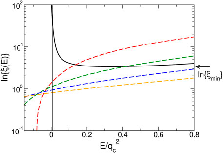
FIGURE 11. Reference conductance, which is proportional to the logarithm of the localization length g₀(E)∝  ln ξ(E) as a function of the spectral parameter $\mathsf{E}/q_c^2={\left[\frac{k_0}{q_c}\right]}^2\sin {(\theta )}^2$. Full (black) line: MT calculation, which gives the same result for all values of k₀. Broken lines: PT calculation for wavelengths λ =2π/k₀ = 1 μm (red) 0.75 μm (green) 0.6 μm (blue) 0.5 μm (orange). The correlation wavenumber has been determined from our samples by image processing to have the value k_c = 8 μm⁻¹ [26]. The arrow indicates the maximum of the distribution of localization lengths in the MT case.

In view of the fact that in our measurement we did not find a dependence on k₀ and that the SCBA of John et al. for the PT approach [67, 71] leads to unphysical results, we suggest that one should rather abandon the PT approach and use the MT one.

3.8 Transverse-Localized Modes and Wavelength Dependence

We stated in the beginning that we experimentally verified [35] that the Anderson-localized wave functions are single modes, i.e., they are single eigenmodes corresponding to a certain eigenvalue ${\mathsf{E}}_i=k_{\perp }^{(i)}$ according to the characteristic equation

${\mathsf{E}}_i{B}_i(x,y,z)=-{\nabla }_{\perp }\frac{M(x,y)}{⟨M⟩}{\nabla }_{\perp }{B}_i(x,y,z)(74)$

For the intensity $I_i(x,y,z)=B_i^2$ steady-state, large z regime is localized around certain spots r_i in the (x, y) plane (see, e.g., Figure 5) and becomes zero on the length scale given by ξ(E_i). As can be seen from Figure 5, the x, y dependence of the wave intensities is rather irregular. Only on the average, we find an exponential decay of the intensity away from r_i.

Let us consider now, in more detail, cases in which one may obtain a wavelength dependence of the localization length. In our experiment, reported in [26] we had a rather large aperture of ∼ 50°. As shown by the authors, this covers the whole ξ(E) spectrum shown in Figure 11 and leads to a ξ distribution peaked at ξ_min, which is k₀ independent. On the other hand, if one would work with a narrow-aperture laser, eventually tilted by a certain angle θ with respect to the optical axis, one could “pick” certain single modes. Because k_⊥ = k₀  sin(θ) has k₀ as prefactor, certainly the mode one may pick up by this procedure will be a different one if k₀ is changed. This opens an interesting method for further investigation of the localized single modes.

3.9 Discussion

In this section we have presented a comprehensive theory of transverse Anderson localization of light. We started to derive the appropriate stochastic Helmholtz equation for electromagnetic waves with spatially fluctuating permittivity. We have shown that the potential-type approach, which is analogous to the Schrödinger equation for an electron in a random potential with the potential depending on the spectral parameter E, relies on an approximation, which is only applicable to very weak disorder, and, for transverse disorder, leads to a wavelength dependence of the localization length. Such a dependence is not observed. In the newly introduced modulus-type approach, which is exact, such a dependence is not predicted, in agreement to our experiments.

Within the modulus-type approach, the localization length, i.e., the radius of the transmitted modes, diverges as the spectral parameter (which is proportional to the square of the azimuthal angle between the direction of the incident radiation and the optical angle) vanishes. This must be so, because a ray in the direction of the optical axis does not experience transverse disorder. The potential-type approach, however, implies a finite mean-free path at zero spectral parameter, and the predicted spectrum penetrates into the negative range of E, rendering the predicted spectrum unstable.

At the end of this section, we would like to comment on the possibility of observing localization of light in three-dimensional systems. As mentioned in the introduction, despite of intensive efforts, this has not been observed until now. We emphasized that the modulus-type theory is analogous to sound waves in solids with spatially fluctuating shear modulus. There it is known that localized states exist at the upper band edge, which in solids is the Debye frequency. In turbid media the analogue of the upper band edge is the inverse of the correlation length of the disorder fluctuations. So if it would be possible to prepare materials with spatial fluctuations of the dielectric modulus, which have a correlation length of the order of the light wavelength, we expect chances for observing 3-dimensional Anderson localization.

4 Nonclassical Anderson Localization of Light

According to the seminal studies by Anderson regarding single-particle evolution in lattices, the disorder in the system leads to localization of the wave-function. As we have illustrated in the first sections, such a phenomenon is well explained by quantum mechanics in the case of electrons and by classical electrodynamics in the case of light in the classical limit; i.e., no quantum effects are involved. In particular, localization is the result of constructive and destructive interference among the multiple paths of the particle. Being an explicit example of the wave-like behavior of quantum particles, the observation of AL in single-photon states does not display any substantial difference with respect to the experiments carried out with classical light. However, single-photons are one of the most promising candidates for quantum information processing in the context of computation, simulation, and cryptography [94]. In this framework, AL has been extensively investigated in photonic quantum walks [95–98]. The latter are versatile platforms for several tasks [99, 100], including simulation of quantum transport effects such as the AL. Furthermore, localized single-photons have been used as a resource to realize quantum cryptography protocols [101, 102]. The investigation of AL at the single-particle level reveals distinctive features when particle-particle interference is taken into accounts [103, 104]. This occurs when more than one particle evolve in the disordered lattice. In this case, other quantum properties of the system, such as particle indistinguishability and statistics, play a crucial role in the spatial distribution of the multiphoton wave-function.

This section regarding quantum AL is organized as follows. First, we introduce the quantum walks model and present single-photon experiments in the context of AL. We further provide practical applications of localized single-photon states in quantum cryptography protocols. Second, we illustrate two-photon quantum walks experiments and the effect of particle statistics in the localization.

4.1 Single-Photon Localization

4.1.1 Quantum Walks

The concept of quantum walks (QW) was first formulated as a generalization of classical random walks (RW) [105]. In the discrete-time evolution, the walk is performed by a quantum particle, which lives in a Hilbert space of d levels corresponding to the position in the lattice. In the classical random walk, the walkers go forward or backward according to the result of a coin toss. In the quantum case, the coin toss is a unitary operator that manipulates an additional two-dimensional degree of freedom embedded in the walker. Then the state of a quantum walker is described by the eigenstates of the position operator w = {|d>} and by the coin basis c = {|↑>, |↓>}. The evolution is regulated by two operators, the coin$\widehat{\mathcal{C}}$ that performs rotations in the coin subspace and the shift$\widehat{S}$. The latter moves the position of the walkers conditionally to the coin state c according to the following expression:

$\widehat{S}=\sum _d|d+1\rangle \langle d|\otimes |\uparrow \rangle \langle \uparrow |+|d-1\rangle \langle d|\otimes |\downarrow \rangle \langle \downarrow |(75)$

The evolution operator in the discrete-time scenario is the combination of the coin and shift action, namely $U_n={(\widehat{S}\cdot (\widehat{C}\otimes {\widehat{\mathbb{I}}}_w))}^n$, where n is the number of single time-step evolution and ${\widehat{\mathbb{I}}}_w$ is the identity operator in the walker’s position space. It is possible to retrieve the evolution operator through the Hamiltonian $\mathcal{H}$ of the system describing a particle evolving in a lattice as $U(t)=e^{-i\mathcal{H}t}$. In this scenario, it is straightforward to translate the above description to the continuous-time case. The operator $\mathcal{H}$ expresses the interactions among the lattice sites like in an adjacency matrix. The resulting QW evolution U(t) is entirely identified by the $\mathcal{H}$ matrix without the need for defining a coin operator as in the discrete-time case. The main feature of the QW with respect to a RW with an unbiased coin is the distribution of the walker for t → ∞. Such distribution depends on the initial state of the particle and the walker tends to spread towards the far ends of the lattice. This is in contrast to the typical diffusive behaviors of a RW. This discrepancy is due to the superposition principle in quantum mechanics that gives rise to the interference effects typical of waves. The formulation of QWs is very general and feasible for different applications and experimental implementations in the quantum information and quantum computation fields [98, 106, 107]. In particular, the formulation of QWs is very suitable for realization in photonic platforms [108]. In the various experiments of photonic QWs, the dynamic of the walker has been encoded in the degrees of freedom of single photon states, such as the polarization for the coin subspace and, for the walker’s position, the optical path in bulk [109, 110] and integrated interferometers [111–116], the time arrival to the detector [117], the modes supported by a multimode fiber [118], the angular [119–121], and the transverse momentum [122].

The QWs evolution operator can be modified for different tasks. For example, the QWs paradigm has been exploited to observe topological-protected states [108, 123], to simulate systems with nontrivial topology [119, 121] and to engineer high-dimensional quantum states [120]. For what concerns AL in discrete-time QWs, single-photon localization has been investigated by introducing site-dependent disorder in the QW evolution. Such condition is achieved implementing site-dependent coin operators. One example is the coin in the form

${\widehat{C}}_d=\frac{1}{\sqrt{2}}\left(\begin{array}{cc}\hfill e^{i{\varphi }_d^{\uparrow }}\hfill & \hfill 0\hfill \\ \hfill 0\hfill & \hfill e^{i{\varphi }_d^{\downarrow }}\hfill \end{array}\right)\cdot \left(\begin{array}{cc}\hfill 1\hfill & \hfill 1\hfill \\ \hfill 1\hfill & \hfill -1\hfill \end{array}\right),(76)$

where random extracted phase-shifts ${\varphi }_d^{\uparrow (\downarrow )}$ operate locally on the site d thus breaking the transnational symmetry of the systems. In [94] the authors present a discrete-time QWs encoded in the time arrival and polarization of single-photon states. The apparatus comprises two loops of different lengths. At each step, the photons generated by a single-photon source choose the shortest or the longest path according to the polarization state that represents the coin space. The position of the particle is encrypted in time. The coin operators in the expression (Eq. 76) were manipulated to reproduce 1) the ballistic spread of the quantum walker by fixing ${\varphi }_d^{\uparrow (\downarrow )}=0$, 2) Anderson localization (AL) with random extracted phase-shift, and 3) the diffusion regime that resembles the behavior of a classical random walker. This last condition is the result of a dephasing between the two polarizations in Eq. 76 larger than the coherence time of the single-photon packets, which destroys the interference among the paths. This experiment was one of the first proofs of AL at the single-photon level. Another example in this direction is [95]. Here the discrete-time QW was realized through an integrated optical circuit composed by a network of beam-splitters and phase-shifts [124, 125]. Single-photon localization was observed in the output modes of the optical circuit.

There are further examples of single-photon localization regarding continuous-time QWs. They are typically realized exploiting continuous coupling among waveguides arranged in a lattice in photonic chips. In this scenario, the time coordinate is again replaced by the distance z covered during the propagation in the waveguides. The single-photon wave-function is given by the Schrödinger equation [126]:

$-i\frac{\partial {\psi }_d}{\partial z}=c_{d,d}{\psi }_d+c_{d,d-1}{\psi }_{d-1}+c_{d+1,d}{\psi }_{d+1},(77)$

where ψ_d is the single-photon amplitude at the site d and the coefficients c_ij are the couplings among the modes of the lattice that are expressed in the Hamiltonian $\mathcal{H}$. The length of the device and the coupling coefficients can be engineered to observe AL, as shown in the single-photon experiments in [96, 97].

Concerning all mentioned quantum experiments, it is worth noting that the localized single-photon distribution has the same properties as the distribution of localized modes of classical light described in Sections 2, 3. The interest in quantum localization is not restricted only to the pure observation of localized states. In the following section, we illustrate an application of localized single-photon states in quantum cryptography.

4.2 Quantum Cryptography Through Localized Single-Photon States

Quantum computing could undermine the security of some of the current cryptographic protocols. An example is given by the RSA protocol security which is based on the difficulty for a classical computer to find prime factors of large integers, while a quantum computer solves the same problem in polynomial time [127]. This motivates the need for a different approach to come up with a more secure cryptographic procedure. Quantum cryptography is the field of quantum information that has the aim to formulate secure protocols based on the rules of quantum mechanics. In the quantum protocol BB84, two agents, Alice and Bob, exchange a stream of qubits, i.e., quantum states that live in a two-dimensional Hilbert space. Alice randomly chooses to prepare the state according to two possible bases {|↑>, |↓>} and {|+>, |−>}, where $|\pm \rangle =\frac{1}{\sqrt{2}}(|\uparrow \rangle \pm |\downarrow \rangle )$. Bob receives the signal and decides randomly in which basis he measures the qubits. He extracts a stream of bits corresponding to 0 when he measures ↑ (+) and to 1 when he measures ↓ (−). Then, Alice and Bob’s streams of bits cannot correspond to each other when Bob measures on a basis different from Alice’s choice. The two agents compare part of their bit strings and, according to the resulting bit error rate, they can detect an eventual eavesdropper attack and extract a secure key [128]. Variants of this protocols exploit entangled states or high-dimensional states instead of qubits. The latter are a generalization of qubits and describe a particle living in a d-dimensional space. The so-called qudits provide advantages in the amount of the information storage in the state sent to the receiver, and security [129].

Single-photon localized states are examples of qudits, where the d-levels correspond to the positions assumed by the photons. In [100] the authors implement a BB84-inspired protocol using localized states generated by a disordered optical fiber. The experimental setup is similar to the one shown in Figure 12. Alice modulates the single photons obtained by an attenuated laser with a spatial light modulator. In this way, she can choose to send states that localize after propagation in the fiber in either momentum or position at the fiber’s output tip. Bob chooses the basis of the measurement by placing or removing a lens before the single-photon detector. This implementation of the BB84 protocol exploits the quantum duality between the real space and the Fourier space of the lens: a state localized in the first space is indeterminate in the other one and vice versa. The authors prove the feasibility of the protocol using localized single-photon wave-functions even in the experimental conditions. A recent work [101] exploits a similar setup for performing a slight different cryptographic protocol. In this experiment, the information about the basis chosen by Alice is not shared publicly after the communication between the agents. Alice codifies her message and the basis in two different photons that are sent at different random time. At the end of the protocol, Alice and Bob compare the measurements about some random pair of photons, and then they are able to extract a secure key. This protocol offers advantages in terms of sensitivity to noise and resilience to a “photon number splitting” eavesdropper attack.

FIGURE 12

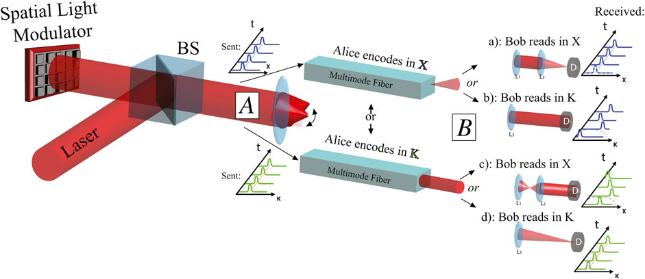
FIGURE 12. Experimental apparatus for quantum cryptography using single-photon localized states. Alice encodes her qudits by preparing single-photon states via a spatial light modulator. She chooses between two bases, namely (K) the eigenstates of the multimode fiber that localize after the propagation and (X) the states that spread after the fiber. Bob measures in the K basis or in the X basis inserting one or two lens before the detection stage. After the comparison between the basis choices by Alice and Bob, they can extract a secure key.

4.3 Multiphoton Localization

Single-photon localized states do not add any further insight into AL with respect to experiments based on wave interference. Nevertheless, the proper description of quantum light is within the framework of second quantization. This representation is necessary for describing many-particle evolution. The electromagnetic field can be expressed by the boson annihilation $\widehat{a}$ and creation operators ${\widehat{a}}^{†}$, i.e., the operators that destroy or create exactly one photon in a given mode [130]. This description reflects the particle statistics and, consequently, explains the quantum interference effects due to the indistinguishability of the particles. This change in the description consists basically in expressing the same state in terms of occupation numbers of the field modes. The system is then individuated by the evolution operator acting to the creation and annihilation operators. In the case of QWs, that, as we have seen in the previous section, corresponds to a linear transformation among modes of a given degree of freedom, the single creation operators representing one photon in the mode i will be

${\widehat{b}}_i^{†}=\sum _j{U}_{ij}{\widehat{a}}_j^{†}(78)$

where U_ij are the element of the QW evolution operator in the occupation number representation. One of the most famous examples of two-photon interference, the Hong-Ou Mandel (HOM) experiment [131] is explained by the latter formulation. Here two indistinguishable photons entering in a beam-splitter from different ports come out always together in the same output port. This phenomenon is a first example of the role of particle indistinguishability in the evolution of multiphoton states.

Two-photon interference has been investigated in the regime of AL. The main result that emerges from these studies is that the way in which the system approaches localization strongly depends on its initial state. In Figure 13 we report numerical simulations illustrating the two-photon state localization investigated in the theoretical [102, 103, 132] and the experimental works [95–97] carried out in this topic. The first row (Figures 13A–D) report the two-photon distribution G (x₁, x₂) defined as the probability to detect one photon in the position x₁ and the other in x₂, averaged over different disorder configurations. For example, in the case two identical photons injected in the QW in positions 0 and 1 in the state $|{\psi }_{in}\rangle ={\widehat{a}}_0^{†}{\widehat{a}}_1^{†}|0\rangle$, the function G (x₁, x₂) has the following expression

$G(x_1,x_2)=⟨⟨|⟨0|{\widehat{a}}_{x_1}{\widehat{a}}_{x_2}|\psi ⟩{|}^2⟩⟩=⟨⟨|U_{x_1,0}{U}_{x_2,1}+U_{x_2,0}{U}_{x_1,1}{|}^2⟩⟩,(79)$

where «⋅» is the average over the disorder, the bra $\langle 0|{\widehat{a}}_{x_1}{\widehat{a}}_{x_2}$ is the projection on the state with the photons in the positions x₁ and x₂ respectively and |ψ> the output state of the QW. The last term is the result of the application of Eq. 78 to the creation operators in the initial state |ψ_in> and of the bosonic operators commutation rule $[a_i,a_j^{†}]={\delta }_{ij}$. The distributions reported in the figure illustrate the state of the system after a discrete-time QW of 30 time steps. In the simulations we have extracted uniformly the phases ${\varphi }_d^{\uparrow (\downarrow )}$ of Eq. 76 around 0 in an interval of length π/2. In such condition, the single-photon wave function still preserves the ballistic spread typical in the QW, while it is starting to localize. In the second row (Figures 13E–H), we show the function $g(\mathrm{\Delta })={\sum }_{x_1-x_2=\mathrm{\Delta }}G(x_1,x_2)$ in the region of localization. All the quantities are normalized to the maximum and averaged among 1,000 configurations of disorder. Figures 13A,B,E,F compare the two functions G and g for the evolution of the initial states ${\widehat{a}}_0^{†}{\widehat{a}}_1^{†}|0\rangle$ and $\frac{1}{\sqrt{2}}({\widehat{a}}_{0,H}^{†}{\widehat{a}}_{1,V}^{†}-{\widehat{a}}_{1,H}^{†}{\widehat{a}}_{0,V}^{†})|0\rangle$. These states correspond to two photons created in the site 0 and 1 with different symmetries with respect to the exchanging operations between the two particles. The first one reproduces the evolution of two noninteracting bosons. Here, we observe the typical tendency of bosons to assume the same states just mentioned in the description of the HOM experiment, i.e., to find the two photons in the same position with high probability. In contrast, the second state is antisymmetric under exchanging of the two particles and presents the opposite behavior. The probability to find the photons in the same site is zero. These states simulate de facto fermion statistics and the Pauli exclusion principle. To reproduce an antisymmetric state, it is necessary to exploit an additional degree of freedom, in this case the polarization. The boson and fermion statistics in AL have been observed experimentally for the first time in [95] by exploiting polarization entangled states and an integrated photonic chip. Here a single-photon source based on parametric down conversion from a nonlinear crystal generates a pair of entangled states in polarization such as the state investigated in Figures 13B,F. The state evolves in a discrete QW platform, realized in an integrated device that comprises a network of beam-splitter and phase-shifts (see Section 4.1). The coin operators in the form of Eq. 76 are sampled properly to observe the AL. The second type of states investigated in the literature is illustrated in Figures 13C,D and g-h. These states are entangled in the occupation number of the sites 0 and 1. The output distribution depends on the sign in the superpositions of the contributions ${{\widehat{a}}^{†2}}_0$ and ${{\widehat{a}}^{†2}}_1$ that create two photons in the respective modes. Such entangled states in the context of AL were investigated for the first time in [96] and then in [97]. The pair of entangled photons is generated via parametric downconversion. These photons are strongly correlated in the momentum space. Such correlations are transferred among the position of the QW’s lattice by means of a lens system. In this way the photons are coupled in the waveguides of the integrated device implementing the QWs. The two experiments with such entangled states have been performed exploiting continuous-time QW by random couplings among the waveguides arranged in a lattice (see Section 4.1). In particular, in the most recent experiment [97], the authors report the results averaged over different configurations of random couplings thus representing one of the most exhaustive experiment on two-photon Anderson localization.

FIGURE 13

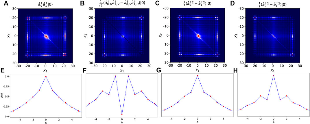
FIGURE 13. Two-photon quantum localization. (A-D) Correlation functions G (x₁, x₂) of a two-photon wave function in a one-dimensional Anderson lattice. The four scenarios report the distributions for different input states in an intermediate time evolution, where the two photons have the same chance to be localized or to spread ballistically. (A) Photons are prepared in a separable state in which they occupy two adjacent sites. (B) Entangled state in the polarization degree of freedom (H: horizontal polarization, V: vertical polarization) that is antisymmetric with respect to the exchange of the particle’s paths. Such state mimics the fermion statistics. Indeed, according to the Pauli exclusion principle, the probability to detect the two photons in the same site is zero. (C,D) Entangled states in the occupation number of two sites. The distribution changes depending by the sign in the superposition. (e,f) The function g(Δ) calculated in the localization area, i.e., x₁, x₂ ∈ [−4,4] and x₁− x₂ = Δ for the four initial states.

4.4 Discussion

In this section we have illustrated Anderson localization (AL) in the context of quantum light, presenting the most relevant results for what concerns the experimental realizations and applications. We have first formulated AL in the context of quantum walks (QW). We have then described the use of localized states in quantum cryptography. In the end we have illustrated the problem of localization in quantum optics by considering multiphoton states. Up to now the investigation of multiphoton AL localization was confined to the two-photon case. The reasons are various. It is still debated in the literature, whether the results reported in the quantum experiments can be reproduced by classical light, i.e., by wave interference. For instance, in [133] it was shown that some features of the distribution reported in Figure 13 could be observed with a laser propagating in a circuit engineered with an appropriate disorder. There are other concerns regarding the intrinsic difficulty to simulate the evolution of noninteracting bosons such as photons scattered by a random network [132]. This prevents finding an analytical solution for the systems with a large number of photons. All these considerations explain why the present investigations about quantum AL were basically carried out from a phenomenological perspective. This motivates further studies to provide a more rigorous framework for quantum AL.

5 Applications and Perspectives

The story understanding transverse localization of light in the last four decades has been one of constant advances. With respect to the first formulations (which reported just numerical evidences [13, 14]), now it is possible to observe and tailor localization on at least four different platforms: photorefractive crystals, plastic binary fibers, disordered glassy fibers, and laser written glass waveguides. Each of this platforms has its specific features and advantages in terms of applications.

1) Photorefractive crystals [134], proposed in 2007, enable relatively rapid reshaping of disorder together with nonlinear response, thus a new generation of switches or routers based on disorder guiding can be envisioned. The drawback of this approach is the small refractive index mismatch and large disorder grain size. For obtaining micron sized localized states, further effort would be needed in improving the nonlinearity engineering.

2) Polymeric binary fibers have been proposed in 2012 and successively further improved. The fabrication technique for these items is extremely cheap and straightforward (if one has access to a fiber drawing tower) and enables realizing kilometer-long fibers starting from a few-centimeter-sized preform. In binary fibers the refractive index mismatch is 0.1 (employing PMMA and Polystyrene as plastic components of the preform), and the disorder can be obtained easily with a grain size of the order of a micron. The advantage of this approach is that the micrometric sized defects need not to be individually fabricated: it is the transverse thinning, affecting collectively all individual strands in the preform that produces this fine-scale disorder. Thus binary fibers support strong localization in the visible range. Binary fibers have been thus extremely successful in terms of potential applications. It has been demonstrated that they can support nonlinearity and switching, image transport, wave front shaping, controlled focusing, quantum communication and key distribution, and image transport. The drawback of binary fibers resides in the large losses: currently between 50 and 100 dB/m. These losses are exceeding the ones expected for the intrinsic scattering and absorption of the plastic material: this poor performance is probably due to the assembly and drawing stage (carried on in a unclean environment), which introduces microscopic dust in the preform. Due to these losses, all the experiments have been carried on longitudinally small pieces of binary fibers (few tens of centimeters).

3) Glass-based binary fibers have been fabricated since 2014 from a porous glass. A rod with initial diameter of 8 mm produces air-holes with diameter varying between 0.2 and 5 µm. This approach promises all the advantages of glass (lower losses and enhanced stability) together with easy fabrication. This potential has already been demonstrated in recent results including new applications such as localization-based random lasing. The only drawback of this approach is related to the nonhomogeneity of the disorder. Indeed, air holes tend to be located at the outer boundary of the fibers due to the fabrication process and, thus, eventually turning localized states into leaky modes.

4) Employing fiber drawing (both in the glassy or plastic versions), it is impossible to get a direct control on the position of the defects. This drawback has been circumvented in 2020, employing a direct laser writing approach. Direct laser writing is still prone to high losses due to inefficient coupling and small refractive index contrast. Nevertheless, by tuning individually the paraxial defect positions, it is possible to test how extensive localization properties depend on specific configurations. Thus direct laser written localization can be employed as a test-bench to find out how different localization properties are affected by varying the disorder configurations. Then, if performance enhancement is found, the optimal configurations can be translated to the more efficient fabrication approaches.

If the technological progress on these platforms continues just at the same rate as in the last years, we can envision that one (or perhaps more than one) of these platforms will find its way to the application and industrialization in the next few years.

Author Contributions

ML reviewed the experiments carried out with coherent light. WS and GR wrote the theoretical background. TG reviewed the experiments with quantum light. All the authors discussed the structure of the work and contributed to the writing of the paper.

Conflict of Interest

The authors declare that the research was conducted in the absence of any commercial or financial relationships that could be construed as a potential conflict of interest.

Publisher’s Note

All claims expressed in this article are solely those of the authors and do not necessarily represent those of their affiliated organizations, or those of the publisher, the editors, and the reviewers. Any product that may be evaluated in this article, or claim that may be made by its manufacturer, is not guaranteed or endorsed by the publisher.

Acknowledgments

ML acknowledges Fondazione “CON IL SUD,” grant “Brains2south,” Project “LOCALITIS” and “Regione Lazio, grant “Gruppi di ricerca 2020,” and Project “LOCALSCENT.”

Footnotes

¹The theory may be generalized to include strong disorder using the coherent-potential approximation [89]. This theory includes percolative aspects, which may be relevant for TL fibers made of glass.

²The reader, not interested in these details, may continue with the next subsection.

³It is important to note that the “diffusivity” D( p, E) is dimensionless, because the “frequency” p = −iω + ϵ has the dimension of an inverse squared length.

References

1. John S. Electromagnetic Absorption in a Disordered Medium Near a Photon Mobility Edge. Phys Rev Lett (1984) 53:2169–72. 10.1103/physrevlett.53.2169.

CrossRef Full Text | Google Scholar

2. Anderson PW. The Question of Classical Localization A Theory of white Paint? Philosophical Mag B (1985) 52:505–9. doi:10.1080/13642818508240619

CrossRef Full Text | Google Scholar

3. Albada MPV, Lagendijk A. Observation of Weak Localization of Light in a Random Medium. Phys Rev Lett (1985) 55:2692–5. doi:10.1103/physrevlett.55.2692

PubMed Abstract | CrossRef Full Text | Google Scholar

4. Wolf P-E, Maret G. Weak Localization and Coherent Backscattering of Photons in Disordered media. Phys Rev Lett (1985) 55:2696–9. doi:10.1103/physrevlett.55.2696

PubMed Abstract | CrossRef Full Text | Google Scholar

5. Akkermans E, Wolf PE, Maynard R. Coherent Backscattering of Light by Disordered media: Analysis of the Peak Line Shape. Phys Rev Lett (1986) 56:1471–4. doi:10.1103/PhysRevLett.56.1471

PubMed Abstract | CrossRef Full Text | Google Scholar

6. Wiersma DS, Bartolini P, Lagendijk A, Righini R. Localization of Light in a Disordered Medium. Nature (1997) 390:671–3. doi:10.1038/37757

CrossRef Full Text | Google Scholar

7. Störzer M, Gross P, Aegerter CM, Maret G. Observation of the Critical Regime Near anderson Localization of Light. Phys Rev Lett (2006) 96:063904. doi:10.1103/PhysRevLett.96.063904

PubMed Abstract | CrossRef Full Text | Google Scholar

8. Sperling T, Bührer W, Aegerter CM, Maret G. Direct Determination of the Transition to Localization of Light in Three Dimensions. Nat Photon (2012) 7:48–52. doi:10.1038/nphoton.2012.313

CrossRef Full Text | Google Scholar

9. Scheffold F, Lenke R, Tweer R, Maret G. Localization or Classical Diffusion of Light? Nature (1999) 398:206–7. doi:10.1038/18347

CrossRef Full Text | Google Scholar

10. Sperling T, Schertel L, Ackermann M, Aubry GJ, Aegerter CM, Maret G. Can 3D Light Localization Be Reached in’white Paint'? New J Phys (2016) 18:013039. doi:10.1088/1367-2630/18/1/013039

CrossRef Full Text | Google Scholar

11. Skipetrov SE, Page JH. Red Light for Anderson Localization. New J Phys (2016) 18:021001. doi:10.1088/1367-2630/18/2/021001

CrossRef Full Text | Google Scholar

12. Skipetrov SE, Sokolov IM. Absence of anderson Localization of Light in a Random Ensemble of point Scatterers. Phys Rev Lett (2014) 112:023905. doi:10.1103/PhysRevLett.112.023905

PubMed Abstract | CrossRef Full Text | Google Scholar

13. Abdullaev SS, Abdullaev FK. On Light Propagation in a System of Tunnelcoupled Waveguides. Izv Vuz Radiofiz (1980) 23:766.

Google Scholar

14. De Raedt H, Lagendijk A, de Vries P. Transverse Localization of Light. Phys Rev Lett (1989) 62:47–50. doi:10.1103/physrevlett.62.47

PubMed Abstract | CrossRef Full Text | Google Scholar

15. Born M, Wolf E. Principles of Optics: Electromagnetic Theory of Propagation, Interference and Diffraction of Light. Elsevier (2013).

16. Pritchett TM, Trubatch AD. A Differential Formulation of Diffraction Theory for the Undergraduate Optics Course. Am J Phys (2004) 72:1026–34. doi:10.1119/1.1758226

CrossRef Full Text | Google Scholar

17. Anderson PW. Absence of Diffusion in Certain Random Lattices. Phys Rev (1958) 109:1492–505. doi:10.1103/physrev.109.1492

CrossRef Full Text | Google Scholar

18. Karbasi S, Mirr CR, Yarandi PG, Frazier RJ, Koch KW, Mafi A. Observation of Transverse anderson Localization in an Optical Fiber. Opt Lett (2012) 37:2304–6. doi:10.1364/ol.37.002304

PubMed Abstract | CrossRef Full Text | Google Scholar

19. Efremidis NK, Sears S, Christodoulides DN, Fleischer JW, Segev M. Discrete Solitons in Photorefractive Optically Induced Photonic Lattices. Phys Rev E Stat Nonlin Soft Matter Phys (2002) 66:046602. doi:10.1103/PhysRevE.66.046602

PubMed Abstract | CrossRef Full Text | Google Scholar

20. Abrahams E, Anderson PW, Licciardello DC, Ramakrishnan TV. Scaling Theory of Localization: Absence of Quantum Diffusion in Two Dimensions. Phys Rev Lett (1979) 42:673–6. doi:10.1103/physrevlett.42.673

CrossRef Full Text | Google Scholar

21. Kroha J, Soukoulis CM, Wölfle P. Localization of Classical Waves in a Random Medium: A Self-Consistent Theory. Phys Rev B (1993) 47:11093–6. doi:10.1103/physrevb.47.11093

CrossRef Full Text | Google Scholar

22. Schwartz T, Bartal G, Fishman S, Segev M. Transport and anderson Localization in Disordered Two-Dimensional Photonic Lattices. Nature (2007) 446:52–5. doi:10.1038/nature05623

PubMed Abstract | CrossRef Full Text | Google Scholar

23. Chen X, Reichenbach KL, Xu C. Experimental and Theoretical Analysis of Core-To-Core Coupling on Fiber Bundle Imaging. Opt Express (2008) 16:21598–607. doi:10.1364/oe.16.021598

PubMed Abstract | CrossRef Full Text | Google Scholar

24. Karbasi S, Frazier RJ, Koch KW, Hawkins T, Ballato J, Mafi A. Image Transport through a Disordered Optical Fiber Mediated by Transverse anderson Localization. Nat Commun (2014) 5:3362–9. doi:10.1038/ncomms4362

PubMed Abstract | CrossRef Full Text | Google Scholar

25. Karbasi S, Mirr CR, Frazier RJ, Yarandi PG, Koch KW, Mafi A. Detailed Investigation of the Impact of the Fiber Design Parameters on the Transverse anderson Localization of Light in Disordered Optical Fibers. Opt Express (2012) 20:18692. doi:10.1364/oe.20.018692

PubMed Abstract | CrossRef Full Text | Google Scholar

26. Schirmacher W, Abaie B, Mafi A, Ruocco G, Leonetti M. What Is the Right Theory for anderson Localization of Light? an Experimental Test. Phys Rev Lett (2018) 120:067401. doi:10.1103/PhysRevLett.120.067401

PubMed Abstract | CrossRef Full Text | Google Scholar

27. Lahini Y, Avidan A, Pozzi F, Sorel M, Morandotti R, Christodoulides DN, et al. Anderson Localization and Nonlinearity in One-Dimensional Disordered Photonic Lattices. Phys Rev Lett (2008) 100:013906. doi:10.1103/PhysRevLett.100.013906

PubMed Abstract | CrossRef Full Text | Google Scholar

28. Sapienza L, Thyrrestrup H, Stobbe S, Garcia PD, Smolka S, Lodahl P. Cavity Quantum Electrodynamics with anderson-localized Modes. Science (2010) 327:1352–5. doi:10.1126/science.1185080

PubMed Abstract | CrossRef Full Text | Google Scholar

29. Leonetti M, Karbasi S, Mafi A, Conti C. Observation of Migrating Transverse anderson Localizations of Light in Nonlocal media. Phys Rev Lett (2014) 112:193902. doi:10.1103/physrevlett.112.193902

PubMed Abstract | CrossRef Full Text | Google Scholar

30. Leonetti M, Karbasi S, Mafi A, Conti C. Experimental Observation of Disorder Induced Self-Focusing in Optical Fibers. Appl Phys Lett (2014) 105:171102. doi:10.1063/1.4900781

CrossRef Full Text | Google Scholar

31. Abrahams E. 50 Years of Anderson Localization. World Scientific (2010). doi:10.1142/7663

CrossRef Full Text

32. Vynck K, Burresi M, Riboli F, Wiersma DS. Photon Management in Two-Dimensional Disordered media. Nat Mater (2012) 11:1017–22. doi:10.1038/nmat3442

PubMed Abstract | CrossRef Full Text | Google Scholar

33. Liu J, Garcia PD, Ek S, Gregersen N, Suhr T, Schubert M, et al. Random Nanolasing in the anderson Localized Regime. Nat Nanotech (2014) 9:285–9. doi:10.1038/nnano.2014.34

CrossRef Full Text | Google Scholar

34. Abaie B, Mobini E, Karbasi S, Hawkins T, Ballato J, Mafi A. Random Lasing in an anderson Localizing Optical Fiber. Light Sci Appl (2017) 6:e17041. doi:10.1038/lsa.2017.41

PubMed Abstract | CrossRef Full Text | Google Scholar

35. Ruocco G, Abaie B, Schirmacher W, Mafi A, Leonetti M. Disorder-induced Single-Mode Transmission. Nat Commun (2017) 8:14571–6. doi:10.1038/ncomms14571

PubMed Abstract | CrossRef Full Text | Google Scholar

36. Mafi A. Transverse anderson Localization of Light: a Tutorial. Adv Opt Photon (2015) 7:459–515. doi:10.1364/aop.7.000459

CrossRef Full Text | Google Scholar

37. Karbasi S, Hawkins T, Ballato J, Koch KW, Mafi A. Transverse Anderson Localization in a Disordered Glass Optical Fiber. Opt Mater Express (2012) 2:1496–503. doi:10.1364/ome.2.001496

CrossRef Full Text | Google Scholar

38. Bertolotti J. Designing Disorder. Nat Photon (2018) 12:59–60. doi:10.1038/s41566-018-0090-y

CrossRef Full Text | Google Scholar

39. Zhou W, Tong Y, Sun X, Tsang HK. Hyperuniform Disordered Photonic Bandgap Polarizers. J Appl Phys (2019) 126:113106. doi:10.1063/1.5117265

CrossRef Full Text | Google Scholar

40. Milošević MM, Man W, Nahal G, Steinhardt PJ, Torquato S, Chaikin PM, et al. Hyperuniform Disordered Waveguides and Devices for Near Infrared Silicon Photonics. Sci Rep (2019) 9:20338–11. doi:10.1038/s41598-019-56692-5

PubMed Abstract | CrossRef Full Text | Google Scholar

41. Pratesi F, Burresi M, Riboli F, Vynck K, Wiersma DS. Disordered Photonic Structures for Light Harvesting in Solar Cells. Opt Express (2013) 21:A460–A468. doi:10.1364/oe.21.00a460

PubMed Abstract | CrossRef Full Text | Google Scholar

42. Aubry GJ, Froufe-Pérez LS, Kuhl U, Legrand O, Scheffold F, Mortessagne F. Experimental Tuning of Transport Regimes in Hyperuniform Disordered Photonic Materials. Phys Rev Lett (2020) 125:127402. doi:10.1103/PhysRevLett.125.127402

PubMed Abstract | CrossRef Full Text | Google Scholar

43. Gianfrate A, Dominici L, Ballarini D, Sanvitto D, Leonetti M. Transverse Localization of Light in Laser Written Designed Disorder. Appl Phys Lett (2020) 116:071101. doi:10.1063/1.5142161

CrossRef Full Text | Google Scholar

44. Gattass RR, Mazur E. Femtosecond Laser Micromachining in Transparent Materials. Nat Photon (2008) 2:219–25. doi:10.1038/nphoton.2008.47

CrossRef Full Text | Google Scholar

45. Martin L, Di Giuseppe G, Perez-Leija A, Keil R, Dreisow F, Heinrich M, et al. Anderson Localization in Optical Waveguide Arrays with off-diagonal Coupling Disorder. Opt Express (2011) 19:13636–46. doi:10.1364/oe.19.013636

PubMed Abstract | CrossRef Full Text | Google Scholar

46. Stützer S, Kartashov YV, Vysloukh VA, Tünnermann A, Nolte S, Lewenstein M, et al. Anderson Cross-Localization. Opt Lett (2012) 37:1715–7. doi:10.1364/ol.37.001715

PubMed Abstract | CrossRef Full Text | Google Scholar

47. Naether U, Meyer JM, Stützer S, Tünnermann A, Nolte S, Molina MI, et al. Anderson Localization in a Periodic Photonic Lattice with a Disordered Boundary. Opt Lett (2012) 37:485–7. doi:10.1364/ol.37.000485

PubMed Abstract | CrossRef Full Text | Google Scholar

48. Naether U, Kartashov YV, Vysloukh VA, Nolte S, Tünnermann A, Torner L, et al. Observation of the Gradual Transition from One-Dimensional to Two-Dimensional anderson Localization. Opt Lett (2012) 37:593–5. doi:10.1364/ol.37.000593

PubMed Abstract | CrossRef Full Text | Google Scholar

49. Vicencio RA, Cantillano C, Morales-Inostroza L, Real B, Mejía-Cortés C, Weimann S, et al. Observation of Localized States in Lieb Photonic Lattices. Phys Rev Lett (2015) 114:245503. doi:10.1103/physrevlett.114.245503

PubMed Abstract | CrossRef Full Text | Google Scholar

50. Stützer S, Plotnik Y, Lumer Y, Titum P, Lindner NH, Segev M, et al. Photonic Topological anderson Insulators. Nature (2018) 560:461–5. doi:10.1038/s41586-018-0418-2

PubMed Abstract | CrossRef Full Text | Google Scholar

51. Lagendijk A, Tiggelen Bv., Wiersma DS. Fifty Years of Anderson Localization. Phys Today (2009) 62:24–9. doi:10.1063/1.3206091

CrossRef Full Text | Google Scholar

52. Mott NF, Twose WD. The Theory of Impurity Conduction. Adv Phys (1961) 10:107–63. doi:10.1080/00018736100101271

CrossRef Full Text | Google Scholar

53. Vollhardt D, Wölfle P. Anderson Localization Ind. Phys Rev Lett (1980) 45:842–6. doi:10.1103/physrevlett.45.842

CrossRef Full Text | Google Scholar

54. Vollhardt D, Wölfle P. Diagrammatic, Self-Consistent Treatment of the Anderson Localization Problem Ind≤2dimensions. Phys Rev B (1980) 22:4666–79. doi:10.1103/physrevb.22.4666

CrossRef Full Text | Google Scholar

55. Vollhardt D, Wölfle P. Scaling Equations from a Self-Consistent Theory of Anderson Localization. Phys Rev Lett (1982) 48:699–702. doi:10.1103/physrevlett.48.699

CrossRef Full Text | Google Scholar

56. Schäfer L, Wegner F. Disordered System Withn Orbitals Per Site: Lagrange Formulation, Hyperbolic Symmetry, and Goldstone Modes. Z Physik B - Condensed Matter (1980) 38:113–26. doi:10.1007/bf01598751

CrossRef Full Text | Google Scholar

57. McKane AJ, Stone M. Localization as an Alternative to Goldstone's Theorem. Ann Phys (1981) 131:36–55. doi:10.1016/0003-4916(81)90182-2

CrossRef Full Text | Google Scholar

58. Wegner F. The Mobility Edge Problem: Continuous Symmetry and a Conjecture. Z Physik B (1979) 35:207–10. doi:10.1007/bf01319839

CrossRef Full Text | Google Scholar

59. Economou EN, Soukoulis CM. Connection of Localization with the Problem of the Bound State in a Potential Well. Phys Rev B (1983) 28:1093–4. doi:10.1103/physrevb.28.1093

CrossRef Full Text | Google Scholar

60. Economou EN, Soukoulis CM, Zdetsis AD. Localized States in Disordered Systems as Bound States in Potential wells. Phys Rev B (1984) 30:1686–94. doi:10.1103/physrevb.30.1686

CrossRef Full Text | Google Scholar

61. Zdetsis AD, Soukoulis CM, Economou EN, Grest GS. Localization in Two- and Three-Dimensional Systems Away from the Band center. Phys Rev B (1985) 32:7811–6. doi:10.1103/physrevb.32.7811

CrossRef Full Text | Google Scholar

62. MacKinnon A, Kramer B. One-parameter Scaling of Localization Length and Conductance in Disordered Systems. Phys Rev Lett (1981) 47:1546–9. doi:10.1103/physrevlett.47.1546

CrossRef Full Text | Google Scholar

63. MacKinnon A, Kramer B. The Scaling Theory of Electrons in Disordered Solids: Additional Numerical Results. Z Physik B - Condensed Matter (1983) 53:1–13. doi:10.1007/bf01578242

CrossRef Full Text | Google Scholar

64. Pichard JL, Sarma G. Finite Size Scaling Approach to anderson Localisation. J Phys C Solid State Phys (1981) 14:L127–L132 and L 617. doi:10.1088/0022-3719/14/6/003

CrossRef Full Text | Google Scholar

65. Pinski S, Schirmacher W, Römer RA. Anderson Universality in a Model of Disordered Phonons. Europhys Lett (2012) 97:16607. doi:10.1209/0295-5075/97/16007

CrossRef Full Text | Google Scholar

66. Bulka B, Schreiber M, Kramer B. Localization, Quantum Interference, and the Metal-Insulator Transition. Z Physik B - Condensed Matter (1987) 66:21–30. doi:10.1007/bf01312758

CrossRef Full Text | Google Scholar

67. John S, Sompolinsky H, Stephen MJ. Localization in a Disordered Elastic Medium Near Two Dimensions. Phys Rev B (1983) 27:5592–603. doi:10.1103/physrevb.27.5592

CrossRef Full Text | Google Scholar

68. John S. Localization of Light. Phys Today (1991) 44:32–40. doi:10.1063/1.881300

CrossRef Full Text | Google Scholar

69. Pinski SD, Schirmacher W, Whall T, Römer RA. Localization-delocalization Transition for Disordered Cubic Harmonic Lattices. J Phys Condens Matter (2012) 24:405401. doi:10.1088/0953-8984/24/40/405401

PubMed Abstract | CrossRef Full Text | Google Scholar

70. Kirkpatrick TR. Localization of Acoustic Waves. Phys Rev B (1985) 31:5746–55. doi:10.1103/physrevb.31.5746

CrossRef Full Text | Google Scholar

71. John S. Strong Localization of Photons in Certain Disordered Dielectric Superlattices. Phys Rev Lett (1987) 58:2486–9. doi:10.1103/physrevlett.58.2486

PubMed Abstract | CrossRef Full Text | Google Scholar

72. Evers F, Mirlin AD. Anderson Transitions. Rev Mod Phys (2008) 80:1355–417. doi:10.1103/revmodphys.80.1355

CrossRef Full Text | Google Scholar

73. Economou EN, Antoniou PD. Localization and Off-Diatonal Disorder. Sol St Comm (1977) 21:258. doi:10.1016/0038-1098(77)90188-0

CrossRef Full Text | Google Scholar

74. Ishimaru A. Wave Propagation and Scattering in Random media. V (New York: Academic Press (1978).

75. Chakravarty S, Schmid A. Weak Localization: The Quasiclassical Theory of Electrons in a Random Potential. Phys Rep (1986) 140:193–236. doi:10.1016/0370-1573(86)90027-x

CrossRef Full Text | Google Scholar

76. Ashcroft NW, Mermin ND. Solid State Physics. Philadelphia: Saunders College) (1976).

77. Schirmacher W. Thermal Conductivity of Glassy Materials and the "boson Peak". Europhys Lett (2006) 73:892–8. doi:10.1209/epl/i2005-10471-9

CrossRef Full Text | Google Scholar

78. Lee PA, Ramakrishnan TV. Disordered Electronic Systems. Rev Mod Phys (1985) 57:287–337. doi:10.1103/revmodphys.57.287

CrossRef Full Text | Google Scholar

79. Sheng P. Introduction to Wave Scattering, Localization and Mesoscopic Phenomena. Heidelberg: Springer (2006).

80. Wölfle P, Vollhardt D. Self-consistent Theory of Anderson Localization: General Formalism and Applications. Int J Mod Phys B (2010) 24:1526–54. doi:10.1142/s0217979210064502

CrossRef Full Text | Google Scholar

81. Saleh BEA, Teich MC. Fundamentals of Photonics. New York: Wiley (1991). See Chapter 5, Equation (5.2-14).

82. Marruzzo A, Schirmacher W, Fratalocchi A, Ruocco G. Heterogeneous Shear Elasticity of Glasses: the Origin of the Boson Peak. Sci Rep (2013) 3:1407. doi:10.1038/srep01407

PubMed Abstract | CrossRef Full Text | Google Scholar

83. Schirmacher W, Scopigno T, Ruocco G. Theory of Vibrational Anomalies in Glasses. J Non-Crystalline Sol (2015) 407:133–40. doi:10.1016/j.jnoncrysol.2014.09.054

CrossRef Full Text | Google Scholar

84. Rayleigh JWSL. On the Light from the Sky, its Polarization and Colour. Philos Mag (1871) 41:241.

Google Scholar

85. Rayleigh L. XXXIV. On the Transmission of Light through an Atmosphere Containing Small Particles in Suspension, and on the Origin of the Blue of the Sky. Lond Edinb Dublin Philosophical Mag J Sci (1899) 47:375–84. doi:10.1080/14786449908621276

CrossRef Full Text | Google Scholar

86. Jackson JD. Classical Electrodynamics. New York: Wiley (1962).

87. Klemens PG. The thermal Conductivity of Dielectric Solids at Low Temperatures (Theoretical). Proc R Soc Lond A (1951) 208:108–33. doi:10.1098/rspa.1951.0147

CrossRef Full Text | Google Scholar

88. Ganter C, Schirmacher W. Rayleigh Scattering, Long-Time Tails, and the Harmonic Spectrum of Topologically Disordered Systems. Phys Rev B (2010) 82:094205. doi:10.1103/physrevb.82.094205

CrossRef Full Text | Google Scholar

89 Köhler S, Ruocco G, Schirmacher W. Coherent potential approximation for diffusion and wave propagation in topologically disordered systems. Phys. Rev. B (2013) 88:064203. doi:10.1103/physrevb.88.064203

CrossRef Full Text | Google Scholar

90. Abramowitz M, Stegun IA. Handbook of Mathematical Functions with Formulas, Graphs, and Mathematical Tables, 55. US Government printing office) (1964).

91. Schirmacher W, Leonetti M, Ruocco G. Analytical Description of the Transverse anderson Localization of Light. J Opt (2017) 19:045602. doi:10.1088/2040-8986/aa61c0

CrossRef Full Text | Google Scholar

92. Gurarie V, Chalker JT. Bosonic Excitations in Random media. Phys Rev B (2003) 68:134207. doi:10.1103/physrevb.68.134207

CrossRef Full Text | Google Scholar

93. Lück V, Sommer HJ, Zirnbauer MR. Energy Correlations for a Random Matrix Model of Disordered Bosons. J Math Phys (2006) 47:103304.

Google Scholar

94. Flamini F, Spagnolo N, Sciarrino F. Photonic Quantum Information Processing: a Review. Rep Prog Phys (2018) 82:016001. doi:10.1088/1361-6633/aad5b2

PubMed Abstract | CrossRef Full Text | Google Scholar

95. Schreiber A, Cassemiro KN, Potoček V, Gábris A, Jex I, Silberhorn C. Decoherence and Disorder in Quantum Walks: From Ballistic Spread to Localization. Phys Rev Lett (2011) 106:180403. doi:10.1103/PhysRevLett.106.180403

PubMed Abstract | CrossRef Full Text | Google Scholar

96. Crespi A, Osellame R, Ramponi R, Giovannetti V, Fazio R, Sansoni L, et al. Anderson Localization of Entangled Photons in an Integrated Quantum Walk. Nat Photon (2013) 7:322–8. doi:10.1038/nphoton.2013.26

CrossRef Full Text | Google Scholar

97. Di Giuseppe G, Martin L, Perez-Leija A, Keil R, Dreisow F, Nolte S, et al. Einstein-podolsky-rosen Spatial Entanglement in Ordered and anderson Photonic Lattices. Phys Rev Lett (2013) 110:150503. doi:10.1103/physrevlett.110.150503

PubMed Abstract | CrossRef Full Text | Google Scholar

98. Gilead Y, Verbin M, Silberberg Y. Ensemble-averaged Quantum Correlations between Path-Entangled Photons Undergoing anderson Localization. Phys Rev Lett (2015) 115:133602. doi:10.1103/PhysRevLett.115.133602

PubMed Abstract | CrossRef Full Text | Google Scholar

99. Aspuru-Guzik A, Walther P. Photonic Quantum Simulators. Nat Phys (2012) 8:285–91. doi:10.1038/nphys2253

CrossRef Full Text | Google Scholar

100. Harrow AW, Montanaro A. Quantum Computational Supremacy. Nature (2017) 549:203–9. doi:10.1038/nature23458

PubMed Abstract | CrossRef Full Text | Google Scholar

101. Leonetti M, Karbasi S, Mafi A, DelRe E, Conti C. Secure Information Transport by Transverse Localization of Light. Sci Rep (2016) 6:29918. doi:10.1038/srep29918

PubMed Abstract | CrossRef Full Text | Google Scholar

102. Santagati R, Price AB, Rarity JG, Leonetti M. Localization-based Two-Photon Wave-Function Information Encoding. Opt Express (2019) 27:20787–99. doi:10.1364/OE.27.02078720799

PubMed Abstract | CrossRef Full Text | Google Scholar

103. Lahini Y, Bromberg Y, Christodoulides DN, Silberberg Y. Quantum Correlations in Two-Particle anderson Localization. Phys Rev Lett (2010) 105:163905. doi:10.1103/physrevlett.105.163905

PubMed Abstract | CrossRef Full Text | Google Scholar

104. Abouraddy AF, Di Giuseppe G, Christodoulides DN, Saleh BEA. Anderson Localization and Colocalization of Spatially Entangled Photons. Phys Rev A (2012) 86:040302. doi:10.1103/PhysRevA.86.040302

CrossRef Full Text | Google Scholar

105. Ambainis A, Bach E, Nayak A, Vishwanath A, Watrous J. One-Dimensional Quantum WalksProceedings of the Thirty-Third Annual ACM Symposium on Theory of Computing (STOC 01). New York, NY: Association for Computing Machinery. (2001) 37–49. doi:10.1145/380752.380757

CrossRef Full Text | Google Scholar

106. Childs AM. Universal Computation by Quantum Walk. Phys Rev Lett (2009) 102:180501. doi:10.1103/PhysRevLett.102.180501

PubMed Abstract | CrossRef Full Text | Google Scholar

107. Ambainis A. Quantum Walks and Their Algorithmic Applications. Int J Quan Inform. (2003) 01:507–18. doi:10.1142/s0219749903000383

CrossRef Full Text | Google Scholar

108. Manouchehri K, Wang J. Physical Implementation of Quantum Walks. Berlin, Heidelberg: Springer Berlin Heidelberg (2014). doi:10.1007/978-3-642-36014-5

CrossRef Full Text

109. Broome MA, Fedrizzi A, Lanyon BP, Kassal I, Aspuru-Guzik A, White AG. Discrete Single-Photon Quantum Walks with Tunable Decoherence. Phys Rev Lett (2010) 104:153602. doi:10.1103/physrevlett.104.153602

PubMed Abstract | CrossRef Full Text | Google Scholar

110. Geraldi A, Laneve A, Bonavena LD, Sansoni L, Ferraz J, Fratalocchi A, et al. Experimental Investigation of Superdiffusion via Coherent Disordered Quantum Walks. Phys Rev Lett (2019) 123:140501. doi:10.1103/PhysRevLett.123.140501

PubMed Abstract | CrossRef Full Text | Google Scholar

111. Owens JO, Broome MA, Biggerstaff DN, Goggin ME, Fedrizzi A, Linjordet T, et al. Two-photon Quantum Walks in an Elliptical Direct-Write Waveguide Array. New J Phys (2011) 13:075003. doi:10.1088/1367-2630/13/7/075003

CrossRef Full Text | Google Scholar

112. Peruzzo A, Lobino M, Matthews JCF, Matsuda N, Politi A, Poulios K, et al. Quantum Walks of Correlated Photons. Science (2010) 329:1500–3. doi:10.1126/science.1193515

PubMed Abstract | CrossRef Full Text | Google Scholar

113. Sansoni L, Sciarrino F, Vallone G, Mataloni P, Crespi A, Ramponi R, et al. Two-particle Bosonic-Fermionic Quantum Walk via Integrated Photonics. Phys Rev Lett (2012) 108:010502. doi:10.1103/physrevlett.108.010502

PubMed Abstract | CrossRef Full Text | Google Scholar

114. Poulios K, Keil R, Fry D, Meinecke JDA, Matthews JCF, Politi A, et al. Quantum Walks of Correlated Photon Pairs in Two-Dimensional Waveguide Arrays. Phys Rev Lett (2014) 112:143604. doi:10.1103/physrevlett.112.143604

PubMed Abstract | CrossRef Full Text | Google Scholar

115. Preiss PM, Ma R, Tai ME, Lukin A, Rispoli M, Zupancic P, et al. Strongly Correlated Quantum Walks in Optical Lattices. Science (2015) 347:1229–33. doi:10.1126/science.1260364

PubMed Abstract | CrossRef Full Text | Google Scholar

116. Caruso F, Crespi A, Ciriolo AG, Sciarrino F, Osellame R. Fast Escape of a Quantum walker from an Integrated Photonic Maze. Nat Commun (2016) 7:11682. doi:10.1038/ncomms11682

PubMed Abstract | CrossRef Full Text | Google Scholar

117. Schreiber A, Cassemiro KN, Potocek V, Gábris A, Mosley PJ, Andersson E, et al. Photons Walking the Line: A Quantum Walk with Adjustable coin Operations. Phys Rev Lett (2010) 104:050502. doi:10.1103/PhysRevLett.104.050502

PubMed Abstract | CrossRef Full Text | Google Scholar

118. Defienne H, Barbieri M, Walmsley IA, Smith BJ, Gigan S. Two-photon Quantum Walk in a Multimode Fiber. Sci Adv (2016) 2:e1501054. doi:10.1126/sciadv.1501054

PubMed Abstract | CrossRef Full Text | Google Scholar

119. Cardano F, Massa F, Qassim H, Karimi E, Slussarenko S, Paparo D, et al. Quantum Walks and Wavepacket Dynamics on a Lattice with Twisted Photons. Sci Adv (2015) 1:e1500087. doi:10.1126/sciadv.1500087

PubMed Abstract | CrossRef Full Text | Google Scholar

120. Cardano F, D’Errico A, Dauphin A, Maffei M, Piccirillo B, de Lisio C, et al. Detection of Zak Phases and Topological Invariants in a Chiral Quantum Walk of Twisted Photons. Nat Commun (2017) 8:15516. doi:10.1038/ncomms15516

PubMed Abstract | CrossRef Full Text | Google Scholar

121. Giordani T, Polino E, Emiliani S, Suprano A, Innocenti L, Majury H, et al. Experimental Engineering of Arbitrary Qudit States with Discrete-Time Quantum Walks. Phys Rev Lett (2019) 122:020503. doi:10.1103/PhysRevLett.122.020503

PubMed Abstract | CrossRef Full Text | Google Scholar

122. D’Errico A, Cardano F, Maffei M, Dauphin A, Barboza R, Esposito C, et al. Two-dimensional Topological Quantum Walks in the Momentum Space of Structured Light. Optica (2020) 7:108–14. doi:10.1364/OPTICA.365028

CrossRef Full Text | Google Scholar

123. Kitagawa T, Broome MA, Fedrizzi A, Rudner MS, Berg E, Kassal I, et al. Observation of Topologically Protected Bound States in Photonic Quantum Walks. Nat Commun (2012) 3:882. doi:10.1038/ncomms1872

PubMed Abstract | CrossRef Full Text | Google Scholar

124. Reck M, Zeilinger A, Bernstein HJ, Bertani P. Experimental Realization of Any Discrete Unitary Operator. Phys Rev Lett (1994) 73:58–61. doi:10.1103/PhysRevLett.73.58

PubMed Abstract | CrossRef Full Text | Google Scholar

125. Clements WR, Humphreys PC, Metcalf BJ, Kolthammer WS, Walsmley IA. Optimal Design for Universal Multiport Interferometers. Optica (2016) 3:1460–5. doi:10.1364/OPTICA.3.001460

CrossRef Full Text | Google Scholar

126. Bromberg Y, Lahini Y, Morandotti R, Silberberg Y. Quantum and Classical Correlations in Waveguide Lattices. Phys Rev Lett (2009) 102:253904. doi:10.1103/PhysRevLett.102.253904

PubMed Abstract | CrossRef Full Text | Google Scholar

127. [Dataset] Nielsen MA, Chuang I. Quantum Computation and Quantum Information (2002).

128. Bennett CH, Brassard G. Quantum Cryptography: Public Key Distribution and coin Tossing. arXiv preprint arXiv:2003.06557 (2020).

Google Scholar

129. Walborn SP, Lemelle DS, Almeida MP, Ribeiro PH. Quantum Key Distribution with Higher-Order Alphabets Using Spatially Encoded Qudits. Phys Rev Lett (2006) 96:090501. doi:10.1103/PhysRevLett.96.090501

PubMed Abstract | CrossRef Full Text | Google Scholar

130. Loudon R. The Quantum Theory of Light. Oxford, United Kingdom: OUP Oxford (2000).

131. Hong CK, Ou ZY, Mandel L. Measurement of Subpicosecond Time Intervals between Two Photons by Interference. Phys Rev Lett (1987) 59:2044–6. doi:10.1103/PhysRevLett.59.2044

PubMed Abstract | CrossRef Full Text | Google Scholar

132. Lahini Y, Bromberg Y, Shechtman Y, Szameit A, Christodoulides DN, Morandotti R, et al. Hanbury Brown and Twiss Correlations of anderson Localized Waves. Phys Rev A (2011) 84:041806. doi:10.1103/physreva.84.041806

CrossRef Full Text | Google Scholar

133. Aaronson S, Arkhipov A. The Computational Complexity of Linear Optics. Proceedings of the Forty-Third Annual ACM Symposium on Theory of Computing. (STOC '11). New York, NY: Association for Computing Machinery (2011). p. 333–42. doi:10.1145/1993636.1993682

CrossRef Full Text | Google Scholar

134. Segev M, Silberberg Y, Christodoulides DN. Anderson Localization of Light. Nat Photon (2013) 7:197–204. doi:10.1038/nphoton.2013.30

CrossRef Full Text | Google Scholar