Comparative Analysis of Super-Kamiokande Solar Neutrino Measurements and Geological Survey of Israel Radon Decay Measurements

Introduction

This article concerns two questions of physics and solar physics that we consider to be currently unresolved. One is the question of whether the solar neutrino flux is constant or variable. Early suggestions of variability were advanced by Sakurai [1], Bieber et al. [2], Haubold and Gerth [3] and Grandpierre [4], among others. However, speaking in 1989, John Bahcall expressed the opinion that the solar neutrino flux must be constant since (in his view) the Sun’s magnetic field is too weak and too fragmented to lead to detectable variations ([5], p. 173).

In 2003, the Super Kamiokande Observatory (SKO) published data (SK-1) acquired over the time interval 1996.4 to 2001.6 (comprising 358 5-days measurements) together with a brief power-spectrum analysis, claiming to find no evidence of variability [6]. However, subsequent more detailed analyses of the same data revealed evidence of variability ([7‐9]). As we discuss in Analysis of Super-Kamiokande SK-1 Data, each of these analyses took a more complete account of the SKO data than did the Yoo analysis, and all found evidence of an oscillation at or near 9.43 year⁻¹.

The other question germane to this article is that of the constancy (or lack of constancy) of nuclear decay processes. Although it as been generally believed that all nuclear decay processes are time-independent, there have for some time been hints that this may not be strictly correct [10–13].

We have much more information from decay experiments than from neutrino experiments, but the information can be confusing. One can find evidence that a certain set of measurements related to the decay of a certain nuclide appear to exhibit variability (e.g., [13]), but one can also find evidence that another set of measurements of the same or a different nuclide do not exhibit variability (e.g. [14]). Furthermore, two analysts examining the same set of data may come to different conclusions. Kossert and Nahle [15] carried out an experiment at the Physikalisch Technische Bundestalt and concluded that their measurements gave no evidence of variability. Kossert and Nahle kindly made their data available to PS and his colleagues who found evidence of variability [16].

One can also find evidence that a small change in an experiment can lead to a big change in the results. Bellotti et al. [17] examined measurements of radiation associated with the decay of radon in an experiment located in the underground laboratory at Gran Sasso. Their first experiment gave unmistakable evidence of a diurnal variation in the measurements. The experimenters then made a small change in the experiment, replacing air in the experimental chamber with olive oil. The revised experiment showed no evidence of variability.

The goal of the current article is to carry out a comparative analysis of solar neutrino measurements and nuclear decay measurements on the assumption that a pattern found in measurements derived from two or more different experiments is more likely to have robust significance than an oscillation found in just one type of experiment. We shall examine in detail SKO measurements of the solar neutrino flux and GSI measurements of radon decay products. We also take account of recent Baksan Neutrino Observatory (BNO) measurements of polonium decay [18].

We analyze the SKO dataset in Analysis of Super-Kamiokande SK-1 Data-first as analyzed by Yoo [6], then as analyzed by [8]. The latter analysis, which takes fuller account of the available experimental information, yields clear evidence of an oscillation at 9.43 year⁻¹.

The most extensive sequence of β-decay measurements is that derived from the GSI radon-decay experiment, which recorded measurements from three decay-product detectors (two α and one γ) and three environmental detectors (temperature, pressure and supply voltage) every 15 min for the decade 2007–2017 [19, 20]. We show in The Geological Survey of Israel Radon Experiment that analysis of the GSI γ measurements reveals highly significant evidence for an oscillation at 9.43 year⁻¹, among other frequencies.

We discuss the implications for solar physics in section Possible Implications for Physics, and Possible Implications Concerning Dark Matter, followed by a general Discussion.

Analysis of Super-Kamiokande SK-1 Data

The SK-1 dataset [6] comprises 358 lines of measurements acquired in 5-day time bins. Each line lists start time, end time, mean live time, flux measurement, lower error estimate and upper error estimate. A plot of the flux versus mean live time is shown in Figure 1A. Yoo et al. presented a Lomb-Scargle analysis [21, 22] of the flux measurements, assigning each measurement to the mean live time of each time bin. They considered a very wide search band (0.07–72 year⁻¹), which is far wider than would be appropriate for a search for solar rotation, for which we consider a generous search band to be 6–16 year⁻¹. Too wide a search band necessarily leads to an overly pessimistic estimate of the relevant significance level.

FIGURE 1

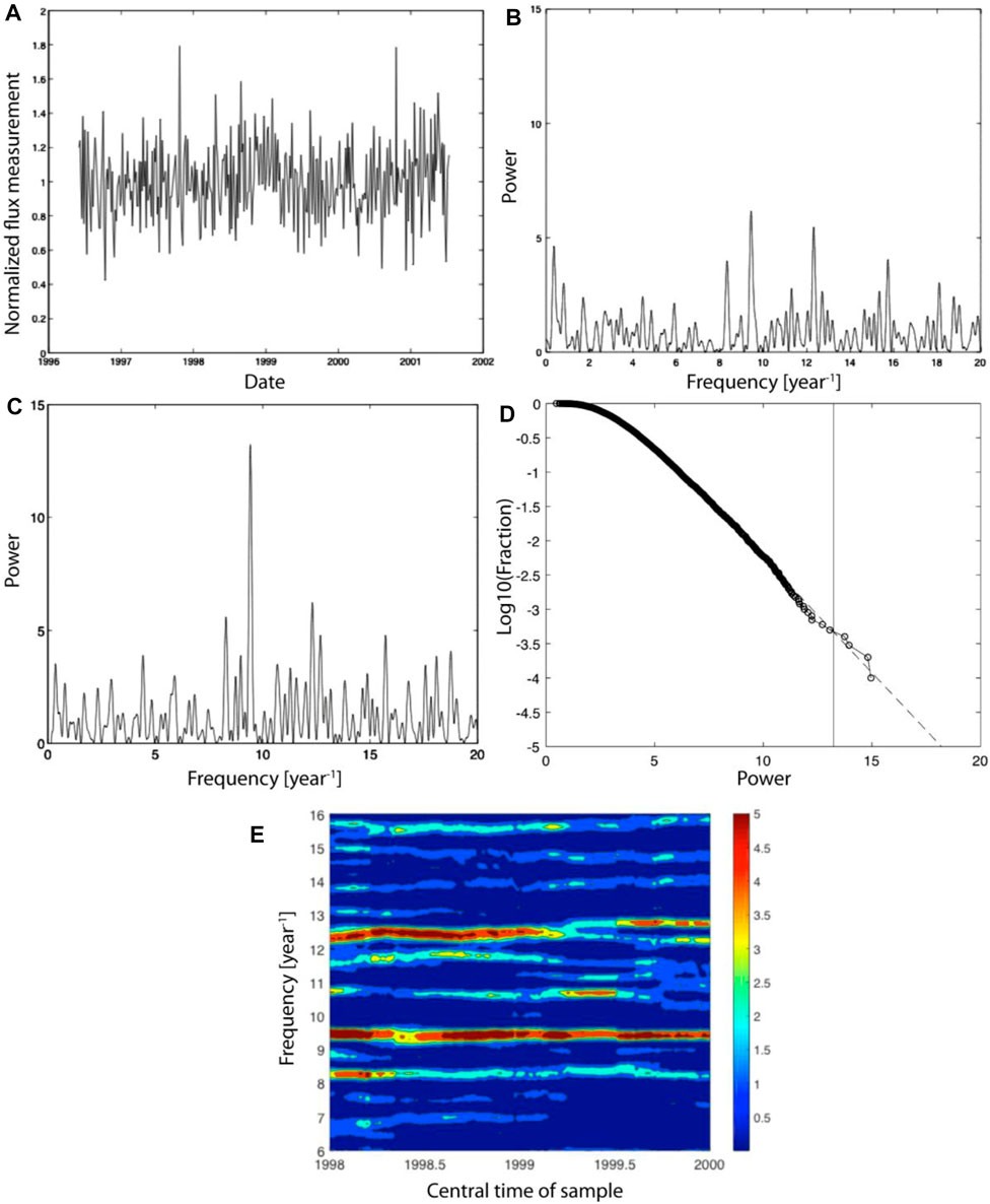
FIGURE 1. (A) Plot of the normalized Super-Kamiokande flux measurements. (The mean flux measurement is $2.33\times {10}^{5}c{m}^{-2}{s}^{-1}$). (B) The Lomb-Scargle power spectrum formed from Super-Kamiokande data, as computed by Yoo et al. (2005), assigning flux measurements to the mean live time of each 5-days bin. (C) Power spectrum formed from Super-Kamiokande data, taking account of start time, end time, flux estimate, lower error estimate and upper error estimate. The strongest peak is at 9.43 year⁻¹, with power 13.24. (D) Shuffle test of the power spectrum formed from Super-Kamiokande data over a unit frequency band (6–7 year⁻¹ chosen, but the choice is unimportant). We find that the probability of finding an oscillation of power 13.24 or more in a band of width 1 year⁻¹ is 4.5 × 10^–4. (E) Spectrogram formed from Super-Kamiokande data, using a “sliding window” of width 2.9 year. The principal features are at 9.4 year⁻¹ and 12.5 year⁻¹, but there is also an interesting feature close to 8.4 year⁻¹.

The Yoo et al. article does not include a table of the results of their power spectrum analysis. However, our reproduction of their analysis [23] yields a peak at 9.43 year⁻¹ with power S = 6.18, which is consistent with Figure 6 of Yoo et al. We shall find that an analysis that takes account of more information yields a more significant result.

For the purpose of power spectrum analysis, we have found it convenient to adopt a date convention that is smoothly running (avoiding leap year; [8]). We first measure dates in “neutrino days” (t_nd) for which January 1, 1970, is adopted as Day 1, and then convert to “neutrino years” by

$t_{n,y}=1970+t_{n,d}/365.2564(1)$

Dates in neutrino years differ from true dates by no more than 1 day.

It is convenient to carry out all power-spectrum analyses by means of a likelihood process [24, 25], since this procedure is flexible enough to be applied to different selections of experimental data. For a single series of measurements (x₁, … , x_N), normalized to have mean value zero, with error estimates ${\sigma }_1,\dots ,{\sigma }_{\mathrm{N}}$ acquired for a single discrete variable (time; t₁, … , t_N), the power S as a function of frequency $v$ is given by

$\begin{array}{l}S\left(\nu \right)=\Sigma \frac{x_n^2}{2}-\Sigma \frac{{\left(x_n-A{e}^{i2\pi t_n}-A^{\ast }{e}^{-i2\pi t_n}\right)}^2}{2}\\ \end{array}(2)$

where, for each value of the frequency $v$, the complex amplitude is adjusted to maximize the likelihood (and hence maximize the power). The maximum value of S may be determined by noting that, at the maximum, the power is stationary with respect to small changes in the complex amplitude:

$\frac{\partial S\left(\nu ,A\right)}{\partial A}=0(3)$

For uniform time steps, and adopting the standard deviation as the error estimate, this equation gives exactly the same result as a simple Fourier analysis. For non-uniform time steps, again adopting the standard deviation as the error estimate, it gives exactly the same power as the Lomb-Scargle procedure [21, 22]. However, it also gives estimates of the complex amplitude A, which converts to amplitude and phase.

Using this likelihood procedure, we may therefore compute the equivalent of a Lomb-Scargle analysis, with the result shown (for the band 0–20 year⁻¹) as Figure 1B. (This plot is identical to that obtained by following the Yoo et al. calculation.)

This basic equation, shown as Equation 2, can be modified for application to measurements recorded for time bins rather than discrete time values, and/or to take account of the upper and lower error estimates for each bin. The result of an analysis that takes account of the start times, end times, lower error estimates, upper error estimates, and flux measurements [8] is shown in Figure 1C, and the powers of the top ten peaks in the search band 6–16 year⁻¹ are listed in Table 1. We see that the most prominent oscillation (at 9.43 year⁻¹) has power 13.24, and the second peak (at 12.31 year⁻¹) has power 6.24.

TABLE 1

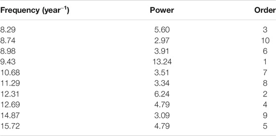
TABLE 1. The top 10 peaks in the frequency band 6–16 year⁻¹ in the power spectrum derived from Super-Kamiokande measurements by a likelihood procedure that takes account of the start time and end time of each bin, the flux estimate at the mean live time, and the upper and lower error estimates.

The standard formula for the probability P of obtaining a peak of power S or more from a normal distribution of fluctuations [22] is given by

$P=e^{-S}(3)$

We see that the probability of finding a peak of power 13.24 or more at a specified frequency is 1.8 × 10^–6.

However, we need to determine the probability of finding by chance a peak of this power or more anywhere in the rotational search band 6–16 year⁻¹, and it would be helpful to be able to consider other possible search bands. If we calculate the probability P₁ of finding a peak of given magnitude (or more) in a band of unit width (1 year⁻¹), we can determine the probability for any other bandwidth B from the equation

$P\left(B\right)=1-{\left(1-e^{-P_1}\right)}^B(4)$

A reliable way to estimate P₁ is by Monte Carlo simulation. We have carried out 10,000 random shuffles of the Super-Kamiokande data, keeping the packages of timing data (start time, end time) unchanged, and keeping the packages of measurements (flux and upper and lower error estimates) unchanged, randomly relating the two sets of packages, and computing the power for each combination. Figure 1D shows as ordinate the fraction of the simulations with a power equal to or larger than the values shown in the abscissa. As expected, the curve tends to an exponential form (e^−S) for large power values, but departs significantly from exponential for small powers. We can read off from the figure the significance value for any power. For S = 13.24 (the actual value for Super-Kamiokande data), we find that there is a probability of 3.6 × 10^–4 of finding by chance an oscillation with that power or more in unit bandwidth. For the narrow band 9.39 year⁻¹ to 9.47 year⁻¹, the probability is found to be 3.0 × 10^–4. For the wide search band 6–16 year⁻¹, the probability becomes 0.003.

The second peak in Table 1, at 12.31 year⁻¹, will be discussed later.

A power spectrum does not show whether an oscillation is steady or transient. However, this can be determined from a spectrogram, formed from a sequence of power calculations for a “moving window.” Such a spectrogram is shown in Figure 1E for the frequency band 6–16 year⁻¹, from which we see that the two principal oscillations, at approximately 9.4 year⁻¹ and 12.3 year⁻¹, are fairly steady. These correspond to the top two peaks listed in Table 1.

The Geological Survey of Israel Radon Experiment

An experiment at the Geological Survey of Israel (GSI) has recorded measurements of γ photons and α particles from radon decay every 15 min from 2007.236 (day 86 of 2007) to 2016.854 (day 312 of 2016) [19, 20].

An excerpt of γ measurements (which have a mean value of 9.424 × 10⁵ per hour) are shown (normalized to mean value unity) in Figure 2A. We see that there is a strong diurnal variation. The variations, as functions of local hour of day and of “hour of year” (dividing the year into 24 parts) are shown in Figures 2B,C, respectively. We see that the variations are of order several percent and are very well defined. (Note that the offsets in the figures are chosen to be ten times the standard error of the mean, to make them distinguishable.)

FIGURE 2

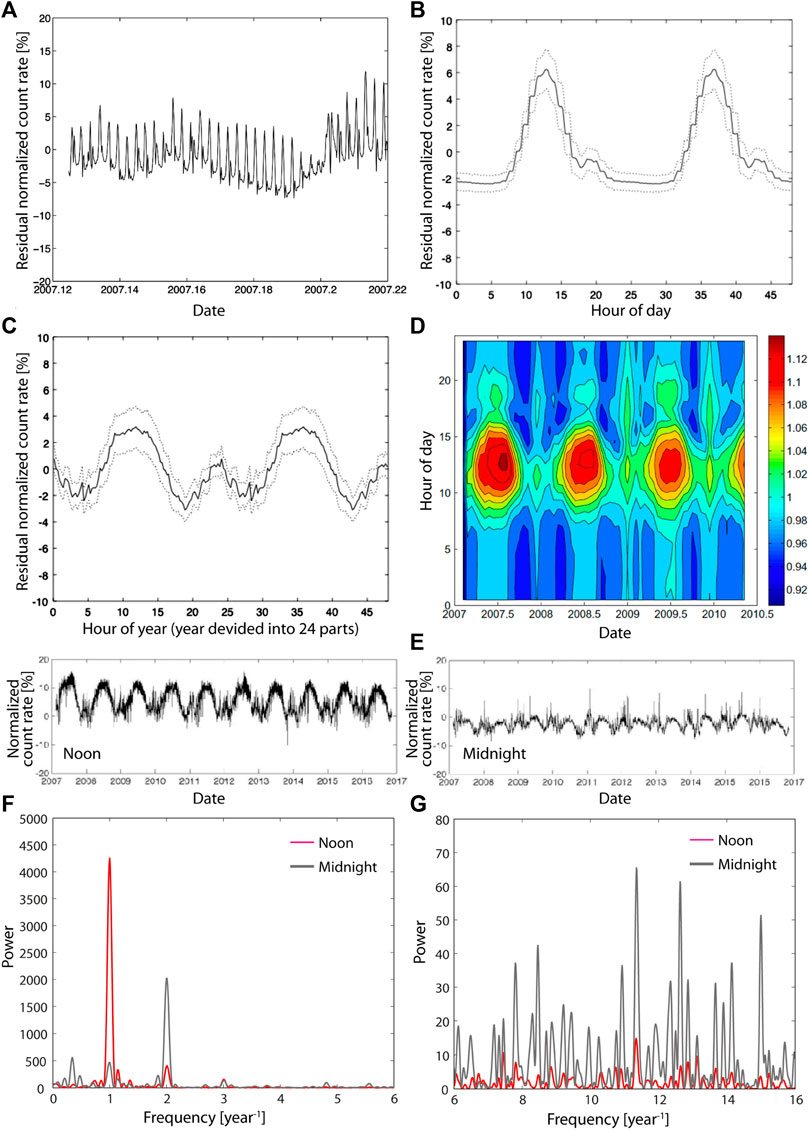
FIGURE 2. (A) Small section of γ measurements, normalized to mean value unity, percent deviation, as a function of time. The sharp fluctuations represent diurnal variations. (B) Residual of normalized γ measurements, in percent, as a function of hour of day (repeated for clarity). The dotted lines indicate the upper and lower offset of ten times the standard error of the mean. (C) Residual of normalized γ measurements, in percent, as a function of hour of year (repeated for clarity). The dotted lines indicate the upper and lower offset of ten times the standard error of the mean. (D) β decay signal as a function of date and hour of day. According to this figure, the dominant contribution to the beta-decay measurements occurs near noon in or near June. Since they are traveling toward the Sun, they can only be cosmic neutrinos. (E) Residuals in percent of the normalized γ measurements made at noon (upper panel, hour of day 11.00–13.00, mean value 5.66%) and at midnight (lower panel, hour of day 23.00 to 1.00, mean value −2.25%) as a function of date. Note that pulses occur only in the midnight data. (F) Power spectra formed from the 4-h band of measurements centered on noon (red) and midnight (blue) for the frequency band 0–6 year⁻¹. We see that the biggest daytime oscillation is at 1 year⁻¹; the biggest nighttime oscillation is at 2 year⁻¹. (G) Power spectra formed from the 4-h band of measurements centered on noon (red) and on midnight (blue) for the frequency band 6–16 year⁻¹. We see that there are strong oscillations in the expected rotational frequency band 10–14 year⁻¹ (note especially the peaks at 11.35 year⁻¹ and 12.64 year⁻¹) in the nighttime data, but comparatively small oscillations in the daytime data. See Table 2 for detected frequencies in the nighttime data.

TABLE 2

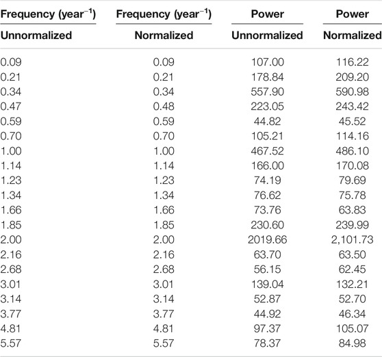
TABLE 2. The frequency and power of the top 20 peaks in power spectra formed from nighttime data for the frequency range 0–6 year⁻¹, as computed from unnormalized data and from rono-normalized data.

In order to distinguish between solar influences and non-solar influences, we find it convenient to examine separately 2 h of measurements centered on local noon and 2 h of measurements centered on local midnight. The resulting plots are shown in Figures 2E–G.

We shall find that the solar influence is found in the midnight data. This already suggests that the β decays are somehow influenced by neutrinos, as has been suggested by several authors (e.g. [11, 12], and [26, 27]). It also suggests that decay products tend to be collimated about the direction of motion of the incident neutrinos.

It is important to note that the GSI experiment is sensitive to the direction of travel of the decay products. The γ detector detects only photons traveling vertically upwards, which is close to the direction of solar neutrinos at midnight. The apparent implication is that neutrinos influence β decays in such a way that, at midnight, neutrinos from the Sun (having traversed the Earth) influence the radon β-decay process. It appears that this interaction is such that decay products tend to travel in the same direction as the incoming neutrinos.

Our tentative identification of midnight measurements with solar neutrinos (to be discussed further) raises the question of the cause of variations in the noon measurements. These variations may be attributed to neutrinos flowing toward the Sun–presumably low-energy galactic neutrinos.

We have carried out power-spectrum analyses of measurements near noon (10 am–2 pm local time) and near midnight (10 pm–2 am local time), with results shown in Figures 2F,G, respectively. The salient peaks for the noon measurements for the frequency range 0–4 year⁻¹ are listed in Table 3, and the salient peaks for the midnight measurements for that frequency range are listed in Table 4. The corresponding tables for the frequency range 6–16 year⁻¹ are listed in Tables 5 and 6.

TABLE 3

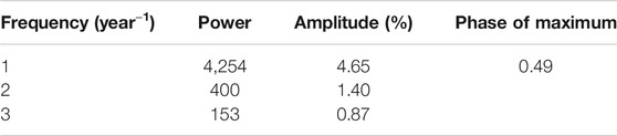
TABLE 3. The annual oscillation and the leading two harmonics as derived from the GSI noon-centered measurements. Table adobted from [28].

TABLE 4

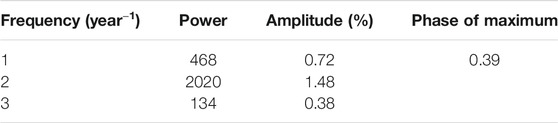
TABLE 4. The annual oscillation and the leading two harmonics as derived from the midnight-centered measurements. Table adobted from [28].

TABLE 5

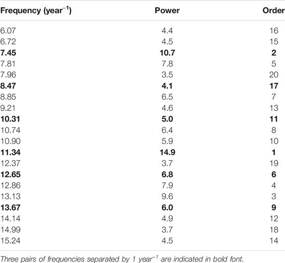
TABLE 5. Top 20 peaks in the power spectrum formed from GSI noon data in the frequency band 6–16 year⁻¹. Table adobted from [28].

TABLE 6

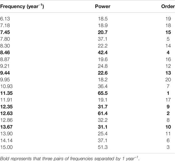
TABLE 6. Top 20 peaks in the power spectrum formed from midnight data in the frequency band 6–16 year⁻¹. Table adobted from [28].

The powers found in the noon measurements are enormous. According to the usual formula for the probability of finding by chance a power of S or more (Equation 3), the significance level of a power of 4,000 is 10^–1740. This formula is based on the assumption that the time-series under investigation has a normal distribution, but it is clear from the figures that this assumption is unlikely to be acceptable for the GSI time series. However, we have shown in a recent article [29] that the significance of non-normality can be checked by a certain operation (the “rono” operation) which converts a non-normal distribution to a normal distribution with the same rank order. We find that there is no significant difference between the power spectrum of the actual data and that of the normalized data.

The main reason the powers are so large is that the time series is so long: 10 years of measurements acquired every hour amount to almost 88,000 lines. A power of 4,000 for a time series of 88,000 lines should be no more surprising than a power of 16 in a similar time series of length 358 lines. This is the length of the Super-Kamiokande dataset, in which we have found an oscillation with power 13.24.

For comparison with the spectrogram formed from Super-Kamiokande measurements, shown as Figure 1E, we now derive spectrograms from GSI measurements by computing the power spectrum of a moving window of length 150 days. We show such spectrograms for the low-frequency band 0–4 year⁻¹ in Figures 3A,B for noon data and midnight data, respectively. We see that these low-frequency oscillations are strong and stable.

FIGURE 3

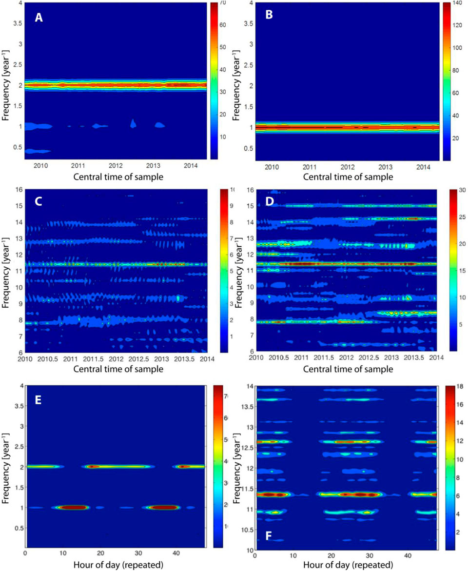
FIGURE 3. (A) Spectrogram formed from noon-time GSI γ measurements, using a sliding window of length 150 days. There is a strong feature at 2 year⁻¹, and a comparatively weak feature at 1 year⁻¹. (B) Spectrogram formed from midnight GSI γ measurements, using a sliding window of length 150 days. There is a strong feature at 1 year⁻¹. (C) Spectrogram formed from noon-time GSI γ measurements, using a sliding window of length 150 days. There is only a weak feature at about 11.4 year⁻¹. (D) Spectrogram formed from midnight GSI γ measurements, using a sliding window of length 150 days. The strongest feature is at about 11.4 year⁻¹. We find weaker transient features at about 9.4 year⁻¹ and 8.4 year⁻¹. (E) Power spectrum as a function of hour of day for the frequency range 0–4 year⁻¹. Note that the dominant feature is an “island” centered on noon at 1 year⁻¹. (F) Power spectrum as a function of hour of day for the frequency range 10–14 year⁻¹. Note that the dominant features are “islands” at frequencies 11.4 year⁻¹ and 12.6 year⁻¹ centered near 3 am.

We show, in Figures 3C,D similar spectrograms for the frequency band 6–16 year⁻¹, derived from noon and midnight data, respectively. Figure 3C, derived from noon measurements, shows little more than a weak feature at 11.3 year⁻¹. By contrast, Figure 3D, derived from midnight data, shows a strong feature at 11.3 year⁻¹, and weaker features at 7.9 year⁻¹, 8.4 year⁻¹, 9.2 year⁻¹ and 12.6 year⁻¹. These features are, as expected, prominent in Table 6.

We also show, in Figures 3E,F, spectrograms that have hour of day and frequency as axes (rather than date and frequency). Figure 3E, which covers the frequency range 0–4 year⁻¹, shows that the annual oscillation occurs mainly near noon, as we expect from Figure 2E, although there is also a strong bi-annual oscillation. By contrast, Figure 3F, which covers the frequency range 10–14 year⁻¹, shows that the dominant oscillations, near 11.4 year⁻¹ and 12.6 year⁻¹, are evident primarily at midnight.

We discuss the implications of these findings for solar physics in Implications for Solar Physics, for physics in Possible Implications for Physics, and Possible Implications Concerning Dark Matter.

Comparison of Super-Kamiokande and Geological Survey of Israel Measurements

We see from Table 1 that the most prominent oscillation in Super-Kamiokande data is found at 9.43 year⁻¹, with power 13.24. We see from Table 6 that essentially the same oscillation occurs in GSI midnight data, with power 22.60 at frequency 9.44 year⁻¹. We see that the same feature appears in both datasets.

We can get an idea of whether or not this correspondence is significant by means of a combined analysis of both power spectra, using procedures designed for such a comparison [30]. We can use the Minimum Power Statistic to search for frequencies for which Super-Kamiokande and GSI both show significant power. One finds that if each power is distributed exponentially, the following function is also distributed exponentially:

$U\left(S_1,S_2\right)=2\ast Min\left(S_1,S_2\right)(5)$

where Min(x,y) indicates the minimum of x and y. This function, formed by combining the Super-Kamiokande power spectrum and the power spectrum formed from midnight GSI measurements, is shown in Figure 4A. Not surprisingly, the peak is found at 9.43 year⁻¹ (with the value U = 26.64).

FIGURE 4

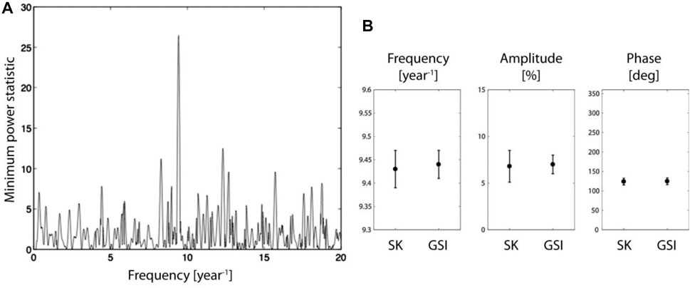
FIGURE 4. (A) The minimum power statistic formed from the Super-Kamiokande power spectrum and the GSI midnight power spectrum. The most significant feature is found at 9.43 year⁻¹, with value 26.64, which could have occurred by chance in the band 0–20 year⁻¹ from normally distributed random noise in both datasets with a probability of 3 × 10^–10. (B) Frequency, amplitude and phase of the 9.43 year⁻¹ oscillation as it appears in Super-Kamiokande measurements and in GSI measurements. A similar version of this subfigure we published already in a previous paper [28].

We may read off the corresponding probability from Eq. 4. According to this equation, there is a probability of e^−22.6, i.e., 1.5 × 10^–10 that this feature could have occurred by chance (from normally distributed random noise) at a specified frequency. Since there are 120 independent peaks in the band 0–20 year⁻¹, there is a probability of 1.8 × 10^–8 of finding by chance a value of U of 26.64 or more in that band.

We have examined this correspondence in more detail by computing the amplitude and phase of each oscillation, with the results shown in Table 7. The correspondence in frequency, amplitude and phase is shown in Figure 4B. For two waveforms that have completely different origins, there appears to be a remarkable consistency, strongly suggestive of a causal relationship.

TABLE 7

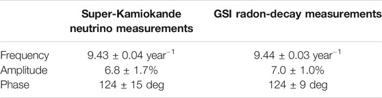
TABLE 7. The frequency, amplitude and phase of the (nominally) 9.43 year⁻¹ oscillation, as it occurs in Super-Kamiokande data and GSI data.

Implications for Solar Physics

The unmistakable difference between measurements made at noon and measurements made at midnight, as seen in Figure 2E, is itself striking proof that the radon measurements are subject to a solar influence. A comparison of the noon and midnight power spectra for the frequency range 6–16 year⁻¹ (appropriate for solar rotation), shown in Figure 2G and in Tables 5 and 6, is further unmistakable evidence. The strongest oscillation noted in Table 6 has a frequency of 12.63 year⁻¹, which is a close fit to the synodic rotation rate of the solar radiative zone as determined by the MDI (Michaelson Doppler Imager) helioseismology experiment on the SOHO (Solar and Heliospheric Observatory) spacecraft [31].

Since radiation measured at midnight has traveled through the Earth, the logical inference is that, as has been suggested by other investigators [11, 12, 27] for other reasons. radon decay measurements are influenced by some form of solar radiation.

This proposal receives unexpected new support from the discovery (noted in Comparison of Super-Kamiokande and Geological Survey of Israel Measurements) of the strikingly close correspondence of the frequency, amplitude and phase of an oscillation at 9.43 year⁻¹ in Super-Kamiokande solar neutrino measurements and GSI radon decay measurements. The agreement of the amplitudes suggests that the variation of the radon decay measurements, in which the 9.43 year⁻¹ variation in embedded, is due entirely (or nearly entirely) to variation of the solar neutrino flux. This is consistent with the fact that this oscillation is most evident in measurements made near midnight, when the experiment is responding primarily to neutrinos arriving from the direction of the Sun.

This interpretation requires that neutrinos can be modulated by some process that is operative in the solar interior so that solar neutrino measurements can be imprinted with oscillations corresponding to a range of internal rotation rates. It is well known that neutrinos can be influenced by both the MSW (Mihkeyev, Smirnov, Wolfenstein) mechanism [32, 33] and the RSFP (Resonant Spin Flavor Precession) mechanism [34, 35]. Since the MSW effect depends only on the composition and density of the solar interior, it will not lead to time variations of the measured neutrino flux, so that it cannot be responsible for oscillations related to solar rotation. On the other hand, the effects of the RSFP mechanism depend on the strength, orientation and structure of the solar internal magnetic field, which presumably vary with location and hence (due to solar rotation) will also vary with time. Hence measurements of radon decay (and other decay) fluctuations are likely to provide information about the dynamic and magnetic properties of the solar interior [36, 37].

We draw attention also the fact that some of the salient periodicities listed in Table 6 have frequencies separated by exactly (or close to exactly) 1 year⁻¹. Such pairings of oscillations are known to be indicative of oblique rotation, i.e. rotation for which the axis is inclined with respect to the normal to the ecliptic [38]. One such pair is 12.63 year⁻¹ (the second strongest oscillation in Table 6) and 13.67 year⁻¹, with powers 61.4 and 31.1 respectively, which (as noted above) may be attributed to the synodic and sidereal rotation frequencies of the radiative zone. Another pair is 11.35 year⁻¹ (the strongest oscillation in Table 6) and 12.35 year⁻¹, with powers 65.5 and 31.7 respectively, which may be suggestive of an “inner radiative zone” situated below the currently known radiative zone.

We note also from Table 6 that the oscillation at or close to 9.43 year⁻¹ is part of a triplet of oscillations: one at 7.45 year⁻¹, one at 8.46 year⁻¹, and the oscillation at 9.44 year⁻¹. If the axis of rotation is inclined at angle $\Theta$ with respect to the normal to the ecliptic, the ratio of the amplitudes of the upper and lower sidebands is given by

$\frac{A\left({\nu }_R+1\right)}{A\left({\nu }_R-1\right)}=\frac{1-\cos \left(\Theta \right)}{1+\cos \left(\Theta \right)}(6)$

where ${\nu }_R$ (year⁻¹) is the sidereal rotation rate, and $\Theta$ is the angle between the rotation axis and the normal to the ecliptic [38]. The powers at 7.45 year⁻¹ and at 9.44 year⁻¹ are similar, which implies that the amplitudes are similar. Since the amplitudes are similar, we are led to consider the possibility that $\Theta \approx \pi /2$, i.e., that this region of the Sun (presumably the core) has a rotation axis almost orthogonal to the normal to the ecliptic, and therefore close to orthogonal to the rotation axis of the photosphere.

There have been independent suggestions that the solar core may be a slow rotator. See, for instance, Elsworth, et al. [39].

Should the core prove to be a slow and oblique rotator, this would point to the possibility that the Sun may have formed in two (or more) distinct stages, and that the core is perhaps the remnant of the first stage.

Possible Implications for Physics

The evidence for variability of GSI radon decay measurements is overwhelming. Such variability is not new, although it is much stronger than noted for other nuclides. Other investigators have found evidence, for other radioactive nuclides, of variability apparently related to the Sun [11, 13]. On the other hand, many experiments at standards laboratories have failed to find significant evidence of variability (see, for instance, [14, 40]). If the variability were to be due to variations in the relevant decay rates, there would appear to be an irreconcilable conflict of evidence. We should note, however, that variability of GSI measurements appears to be highly anisotropic. This points to the possibility that the variability detected by some experiments is due intrinsically to an anisotropy in the radiation, not to a variation in the net radiation. This hypothesis would be compatible with a finding that any experiment that measures only the total radiation (such as a 4π detector) would fail to detect any evidence of variability.

An experiment reported by Bellotti et al. [41] appears to support this conjecture. These investigators first studied γ radiation from the decay of radon in a configuration in which the photons traveled only a short distance in air from the radon nuclei to the NaI radiation detector. With this configuration, measurements exhibited a very strong diurnal variation. The investigators then modified the experiment, first by filling the chamber with polystyrene particles, then with olive oil. With these configurations, the detectors showed no evidence of a diurnal variation. Noting that both the polystyrene particles and the olive oil would tend to isotropize the flux of photons emitted by the radon, these results appear to be compatible with the hypothesis that the relevant variability may be attributed to directionality, not emissivity.

To the best of our knowledge, experiments at standards laboratories that are designed to measure decay rates typically measure radiation from specimens of nuclides that are immersed in some kind of medium, which may tend to isotropize radiation from the nuclide. Although we are aware of experiments that respond to the total radiation from nuclides that fail to show evidence of variability, we are unaware of any experiment that is sensitive to direction of emission that fails to show evidence of variability.

These considerations lead to the following conjecture: Neutrinos have no influence on the decay rate of a radioactive nuclide. However, neutrinos or neutrino-related particles may influence the direction of propagation of radiation associated with decay, if and when decay occurs.

We also offer the following suggestion: the influence of neutrinos on nuclear decay may not be a binary process, by which a single neutrino affects the decay of a single nucleus. It may instead involve a collective influence (similar to collective processes in plasmas) by which a large number of neutrinos may, in a collective process influence the direction of emission of decay products, if and when decay occurs.

Possible Implications Concerning Dark Matter

Alexander Parkhomov, of the Russian Academy of Natural Sciences and the Lomonosov Moscow State University, has carried out research concerning nuclear decays for many years, finding evidence of variability of β decays but not of α decays [26]. Parkhomov [27] has drawn attention to the possibility that β decays may be influenced by “cosmic slow neutrinos,” which may be a contributor to “dark matter.” We explore this possibility in this section.

Figures 2B–D show the β decay signal as a function of date and of hour of day. According to these figures, the dominant contribution to the β decay measurements occurs near noon in or near June. Neutrinos detected near noon are traveling toward the Sun, not from the Sun. These can only be cosmic neutrinos.

This signal matches the expectation for the production of a cosmic influence such as dark matter as estimated by [42], and matches results of the DAMA/Libra dark matter experiment [43], which exhibits a strong peak in early June.

Figure 2B does not show an obvious enhancement at midnight, implying that the solar neutrino flux is smaller than the average neutrino flux by at least a factor of 10. Estimates of the solar neutrino production presented by [44] lead to an estimate for the solar neutrino flux at Earth of

$F\left(\mathrm{solar}\mathrm{neutrinos}\right)={10}^{10.9}c{m}^{-2}{s}^{-1}$(7.1)

(mainly pp neutrinos). This suggests that we consider a cosmic neutrino flux of at least

$F\left(\mathrm{cosmic}\mathrm{neutrinos}\right)={10}^{12}c{m}^{-2}{s}^{-1}$(7.2)

If neutrinos approach the Sun with negligible speed, the speed they will have at the Earth’s orbit is given by

$v\left(\mathrm{infall}\right)={\left(\frac{2G{M}_{solar}}{r}\right)}^{1/2}$(7.3)

With G = 10^–7.18, M = 10^33.30 and r = 1 AU = 10^13.18 (all in cgs units), we find that

$v\left(\mathrm{infall}\right)={10}^{6.6}cm{s}^{-1}$(7.4)

Hence if the local speed of cosmic neutrinos is due to the Sun’s gravitational influence, the cosmic neutrino number density at the Earth’s orbit may be estimated to be

$n_{\nu }=F/v={10}^{4.5}\hspace{0.17em}\mathrm{c}{\mathrm{m}}^{-3}$(7.5)

The cosmic neutrino mass density may then be estimated to be

${\rho }_{\nu }={10}^{4.5}{m}_{\nu }g\mathrm{c}{\mathrm{m}}^{-3}$(7.6)

where $m_{\nu }$ is the neutrino mass in grams.

Gaitskell et al. [45] has estimated the density of cosmic dark matter to be

${\rho }_c={10}^{-28.73}{h}^{2}g\mathit{c}{\mathit{m}}^{-3}$(7.7)

where h is the dimensionless form of the Hubble constant in units of 100 km/s/Mpc.

The current experimental estimate of h is approx. 0.7, leading to an estimate of ${10}^{-29.0}gc{m}^{-3}$ for the density of dark matter. We see from Eq. 7.6 that this requires a mass of 10^–33.5 g, i.e., 0.2 eV, for the neutrino mass.

This estimate is consistent with the upper limit of 1 eV for the neutrino mass, as determined by the Katrin experiment [46]. It therefore appears that galactic neutrinos may be able to supply the mass of dark matter at least on a local scale.

Discussion

This article has been concerned with the following questions:

1. Is the solar neutrino flux constant or variable?

2. Are radon decay products constant or variable?

3. If both are variable, are the variations related?

Analysis of Super-Kamiokande SK-1 Data presented evidence that the solar neutrino flux is indeed variable, the variability being most evident in an oscillation with frequency 9.43 year⁻¹.

The Geological Survey of Israel Radon Experiment presented evidence that radon decay products are highly variable with very strong diurnal and annual oscillations, but also with evidence for oscillations in a frequency band appropriate for solar rotation.

In Comparison of Super-Kamiokande and Geological Survey of Israel Measurements, we found evidence for a correspondence between oscillations in solar neutrino measurements and in radon decay-product measurements: namely a common oscillation with frequency 9.43 year⁻¹. Not only do those data sets both exhibit an oscillation at that frequency, there is a remarkable agreement in the amplitudes and phases of these two completely different data sets.

Hence evidence in this article points toward an association between variations in the solar neutrino flux and variations in radon decay products. Such an association, if real, is suggestive of an influence of neutrinos on the decay process. However, it may not be a direct influence. It is possible that the interaction is mediated by another particle or field (possibly a boson), just as the influence of ions on electrons in a plasma is mediated by the electromagnetic field.

Of the two data sets, the radon set provides by far the most information. (We have examined only a quarter of the 350,000 lines.) In particular, it provides a rich power spectrum for a frequency range appropriate for solar rotation.

There are several pairs of oscillations in GSI measurements with frequencies separated by 1 year⁻¹, which are indicative of an influence of rotation about an axis that is not parallel to the normal to the ecliptic [37]. The oscillations at effectively 12.66 year⁻¹ and 13.66 year⁻¹ match the synodic and sidereal rotation frequencies of the solar radiative zone. A triplet of oscillations with frequencies at or close to 7.43 year⁻¹, 8.43 year⁻¹ and 9.43 year⁻¹ is suggestive of a region that rotates with a sidereal frequency of 8.43 year⁻¹ about an axis that is almost orthogonal to the normal to the ecliptic. We suggest that this region is the solar core. Such a finding, if it proves correct, may call for a revision of our concepts concerning the formation, structure and evolution of the Sun.

We now call attention to an experiment at the Baksan Neutrino Observatory, as reported by Alexeyev et al. [18]. This also is an experiment to study nuclear decays, but it is quite different from experiments of the type of the BNL (Brookhaven National Laboratory) experiment [10, 25] and quite different from the GSI experiment. It measures the decay of ²¹⁴Po (half-life: 163 µs) (TAU-1 and TAU-2 installation; [47, 48]) and ²¹³Po (half-life: 4.2 µs) (TAU-3 installation) [17]. The decay of ²¹³Po is prompted by the decay of ²¹³Bi, which has a half-life of 46 min and decays by the β process, emitting both an electron and a photon. Since the timing of the ²¹³Po decay is related to the detection of the ²¹³Bi decay products, measurements of the ²¹³Po decay process may be influenced by complications attendant on the decay of ²¹³Bi.

For our purposes the crucial point is that measurement of the decay of ²¹³Po gives clear evidence of an oscillation with frequency 9.43 year⁻¹ (see Figure 5). Due to the complication of the initiation of the α decay of ²¹³Po by the termination of the ²¹³Bi β decay, the apparent variability of ²¹³Po α decay may in part reflect variability of ²¹³Bi β decay.

FIGURE 5

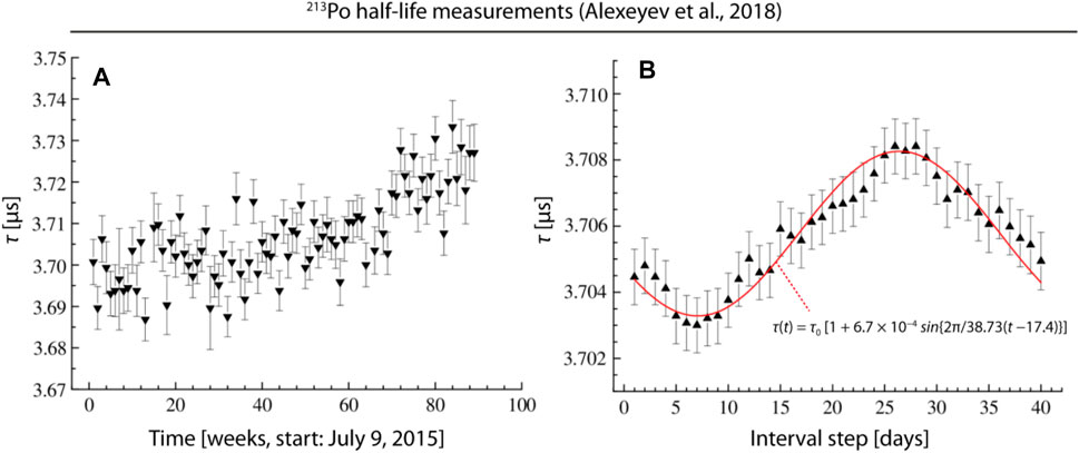
FIGURE 5. ²¹³Po half-life measurements at BNO. (A) Time-dependence of half-life values of ²¹³Po. Weekly data. (B) Detection of an oscillation in the ²¹³Po half-life data with a period of 9.43 year⁻¹ (period of 38.73 days) using the method of interior moving average with a one-day step. Reprinted with modifications from Alexeyev et al. [17] (picture obtained from the arXiv version of the article, arXiv:1806.01152).

Nevertheless, whatever the detailed association between the decay of ²¹³Po and the decay of ²¹³Bi, the BNO experiment shows that, in addition to evidence of the 9.43 year⁻¹ oscillation in both SKO measurements and GSI measurements, there is supporting evidence from a third experiment–the BNO ²¹³Po experiment.

Data Availability Statement

The original contributions presented in the study are included in the article/Supplementary Files, further inquiries can be directed to the corresponding author.

Author Contributions

PS wrote the first draft of the article. OP provided the GSI data. FS revised the mansucript and helped in creating the figures.

Conflict of Interest

The authors declare that the research was conducted in the absence of any commercial or financial relationships that could be construed as a potential conflict of interest.

Publisher’s Note

All claims expressed in this article are solely those of the authors and do not necessarily represent those of their affiliated organizations, or those of the publisher, the editors and the reviewers. Any product that may be evaluated in this article, or claim that may be made by its manufacturer, is not guaranteed or endorsed by the publisher.

Acknowledgments

We thank Jeffrey Scargle and Guenther Walther for their helpful comments and suggestions concerning statistical issues that have arisen in the course of this project. We thank Daniel Freedman for helpful discussions concerning particle physics issues.

References

1. Sakurai K. Quasi-Biennial Periodicity in the Solar Neutrino Flux and its Relation to the Solar Structure. Solar Phys (1981) 74:35–41. doi:10.1007/978-94-010-9633-1_5

CrossRef Full Text | Google Scholar

2. Bieber JW, Seckel D, Stanev T, Steigman G. Variation of the Solar Neutrino Flux with the Sun's Activity. Nature (1990) 348:407–11. doi:10.1038/348407a0

CrossRef Full Text | Google Scholar

3. Haubold HJ, Gerth E. On the Fourier Spectrum Analysis of the Solar Neutrino Capture Rate. Sol Phys (1990) 127:347–56. doi:10.1007/bf00152173

CrossRef Full Text | Google Scholar

4. Grandpierre A. A Pulsating-Ejecting Solar Core Model and the Solar Neutrino Problem. Astron Astrophys (1996) 308:1996.

Google Scholar

5. Sturrock PA. The Life and Times of a Dissident Scientist. Sol Phys (2017) 292:147. doi:10.1007/s11207-017-1156-6

CrossRef Full Text | Google Scholar

6. Yoo J. Search for Periodic Modulations of the Solar Neutrino Flux in Super-kamiokande-1. Phys Rev D (2003) 68:092002.

Google Scholar

7. Ranucci G. Likelihood Scan of the Super-kamiokande I Time Series Data. Phys Rev D (2006) 73:103003. doi:10.1103/physrevd.73.103003

CrossRef Full Text | Google Scholar

8. Sturrock PA, Scargle JD. Power-Spectrum Analysis of Super-Kamiokande Solar Neutrino Data, Taking into Account Asymmetry in the Error Estimates. Solar Phy. (2006) 237:1–11.

9. Caldwell DO. Evidence for Sterile Neutrinos Which Could Be Part of Dark Matter. Nucl Phys B - Proc Supplements (2007) 173:36–9. doi:10.1016/j.nuclphysbps.2007.08.102

CrossRef Full Text | Google Scholar

10. Alburger DE, Harbottle G, Norton EF. Half-life of 32Si. Earth Planet Sci Lett (1986) 78:168–76. doi:10.1016/0012-821x(86)90058-0

CrossRef Full Text | Google Scholar

11. Falkenberg ED. Radioactive Decay Caused by Neutrinos? Apeiron (2001) 8(No. 2):32.

Google Scholar

12. Fischbach E, Buncher JB, Gruenwald JT, Jenkins JH, Krause DE, Mattes JJ, et al. Time-Dependent Nuclear Decay Parameters: New Evidence for New Forces? Space Sci Rev (2009) 145:285–335. doi:10.1007/s11214-009-9518-5

CrossRef Full Text | Google Scholar

13. Jenkins JH, Fischbach E, Buncher JB, Gruenwald JT, Krause DE, Mattes JJ. Evidence of Correlations between Nuclear Decay Rates and Earth-Sun Distance. Astroparticle Phys (2009) 32:42–6. doi:10.1016/j.astropartphys.2009.05.004

CrossRef Full Text | Google Scholar

14. Pommé S, Stroh H, Paepen J, Van Ammel R, Marouli M, Altzitzoglou T, et al. Evidence against Solar Influence on Nuclear Decay Constants. Phys Lett B (2016) 761:281–6. doi:10.1016/j.physletb.2016.08.038

PubMed Abstract | CrossRef Full Text | Google Scholar

15. Kossert K, Nähle OJ. Long-term Measurements of 36Cl to Investigate Potential Solar Influence on the Decay Rate. Astroparticle Phys (2014) 55:33–6. doi:10.1016/j.astropartphys.2014.02.001

CrossRef Full Text | Google Scholar

16. Sturrock PA, Fischbach E, Scargle JD. Comparative Analyses of Brookhaven National Laboratory Nuclear Decay Measurements and Super-kamiokande Solar Neutrino Measurements: Neutrinos and Neutrino-Induced Beta-Decays as Probes of the Deep Solar Interior. Sol Phys (2016) 291:3467–84. doi:10.1007/s11207-016-1008-9

CrossRef Full Text | Google Scholar

17. Bellotti E, Broggini C, Di Carlo G, Laubenstein M, Menegazzo R. Search for Time Dependence of the 137Cs Decay Constant. Phys Lett B (2012) 710:114–7. doi:10.1016/j.physletb.2012.02.083

CrossRef Full Text | Google Scholar

18. Alexeyev EN, Gavrilyuk YM, Gangapshev AM. Search for Variations of ²¹³Po Half-Life. Phys Particles Nuclei (2018) 49(4):557–62.

Google Scholar

19. Steinitz G, Piatibratova O. Report GSI/17/2008, Geological Survey of Israel (2008). Available from: https://www.researchgate.net/publication/264120472_Experimental_replication_of_radon_signals_that_occur_in_the_geological_environment (Accessed 2008).

Google Scholar

20. Steinitz G, Piatibratova O, Kotlarsky P. Possible Effect of Solar Tides on Radon Signals. J Environ Radioactivity (2011) 102:749–65. doi:10.1016/j.jenvrad.2011.04.002

CrossRef Full Text | Google Scholar

21. Lomb NR. Least-squares Frequency Analysis of Unequally Spaced Data. Astrophys Space Sci (1976) 39:447–62. doi:10.1007/bf00648343

CrossRef Full Text | Google Scholar

22. Scargle JD. Studies in Astronomical Time Series Analysis. II - Statistical Aspects of Spectral Analysis of Unevenly Spaced Data. ApJ (1982) 263:835. doi:10.1086/160554

CrossRef Full Text | Google Scholar

23. Sturrock PA, Steinitz G, Fischbach E, Parkhomov A, Scargle JD. Analysis of Beta-Decay Data Acquired at the Physikalisch-Technische Bundesanstalt: Evidence of a Solar Influence. Astroparticle Phys (2016) 84:8–14. doi:10.1016/j.astropartphys.2016.07.005

CrossRef Full Text | Google Scholar

24. Sturrock PA, Walther G, Wheatland MS. Search for Periodicities in the Homestake Solar Neutrino Data. ApJ (1997) 491:409–13. doi:10.1086/304955

CrossRef Full Text | Google Scholar

25. Sturrock PA, Caldwell DO, Scargle JD. Power-spectrum Analyses of Super-kamiokande Solar Neutrino Data: Variability and its Implications for Solar Physics and Neutrino Physics. Phys Rev D (2005) 72:11300. doi:10.1103/physrevd.72.113004

CrossRef Full Text | Google Scholar

26. Parkhomov AG. Deviations from Beta Radioactivity Exponential Drop. Jmp (2011) 02:1310–7. doi:10.4236/jmp.2011.211162

CrossRef Full Text | Google Scholar

27. Parkhomov AG. Rhythmic and Spоradic Changes in the Rate of Beta Decays: Possible Reasons. Jmp (2018) 09:1617–32. doi:10.4236/jmp.2018.98101

CrossRef Full Text | Google Scholar

28. Sturrock PA, Scholkmann F. Possible Indications of Variations in the Directionality of Beta-Decay Products. Front Phys (2021) 8:584101. doi:10.3389/fphy.2020.584101

CrossRef Full Text | Google Scholar

29. Sturrock P, Scholkmann F. The RONO (Rank-Order-Normalization) Procedure for Power-Spectrum Analysis of Datasets with Non-Normal Distributions. Algorithms (2020) 13:157. doi:10.3390/a13070157

CrossRef Full Text | Google Scholar

30. Sturrock PA, Scargle JD, Walther G, Wheatland MS. Combined and Comparative Analysis of Power Spectra. Sol Phys (2005) 227:137–53. doi:10.1007/s11207-005-7424-x

CrossRef Full Text | Google Scholar

31. Schou J, Antia HM, Basu S, Bogart RS, Bush RI, Chitre SM, et al. Helioseismic Studies of Differential Rotation in the Solar Envelope by the Solar Oscillations Investigation Using the Michelson Doppler Imager. ApJ (1998) 505:390–417. doi:10.1086/306146

CrossRef Full Text | Google Scholar

32. Mikheev SP, Smirnov I. Resonance Enhancement of Oscillations in Matter and Solar Neutrino Spectroscopy. Nuovo Cimento C9 (1986) 17.

Google Scholar

33. Wolfenstein L. Neutrino Oscillations in Matter. Phys Rev D (1978) 17:2369–74. doi:10.1103/physrevd.17.2369

CrossRef Full Text | Google Scholar

34. Akhmedov EK. Resonant Amplification of Neutrino Spin Rotation in Matter and the Solar-Neutrino Problem. Phys Lett B (1988) 213:64–8. doi:10.1016/0370-2693(88)91048-9

CrossRef Full Text | Google Scholar

35. Ahmedov RK, Lanza A, Petcov ST. Solar Neutrino Data, Neutrino Magnetic Moments and Flavor Mixing. Phys Lett B (1995) 348:124.

Google Scholar

36. Pulido J. The Solar Neutrino Problem and the Neutrino Magnetic Moment. Phys Rep (1992) 211:167–99. doi:10.1016/0370-1573(92)90071-7

CrossRef Full Text | Google Scholar

37. Sturrock PA, Fischbach E, JavorsekII D, Jenkins JH, Lee RH. The Case for a Solar Influence on Certain Nuclear Decay Rates. (2013). arXiv:1301.3754.

Google Scholar

38. Sturrock PA, Bai T. Search for Evidence of a Clock Related to the Solar 154 Day Complex of Periodicities. ApJ (1992) 397:337. doi:10.1086/171789

CrossRef Full Text | Google Scholar

39. Elsworth Y, Howe R, Isaak GR, McLeod CP, Miller BA, New R, et al. Slow Rotation of the Sun's interior. Nature (1995) 376:669–72. doi:10.1038/376669a0

CrossRef Full Text | Google Scholar

40. Pomme S, Lutter G, Marouli M. On the Claim of Modulations in Radon Data and Their Association with Solar Rotation. Astropart Phys (2017) 97:38.

Google Scholar

41. Bellotti E, Broggini C, Broggini C, Di Carlo G, Laubenstein M, Menegazzo R. Precise Measurement of the 222Rn Half-Life: A Probe to Monitor the Stability of Radioactivity. Phys Lett B (2015) 743:526–30. doi:10.1016/j.physletb.2015.03.021

CrossRef Full Text | Google Scholar

42.Freese. Status of dark matter in the universe, The Fourteenth Marcel Grossmann Meeting. (2017) 325–355.

43. Bernabei R, Belli P, Bussolotti A, Cappella F, Caracciolo V, Cerulli R, et al. First Model Independent Results from DAMA/LIBRA–Phase2. Universe (2018) 4:116. doi:10.3390/universe4110116

44. Bahcall JN. Neutrino Astrophysics. Cambridge University Press (1989)

45. Gaitskell RJ. Direct detection of dark matter. Annu. Rev. Nucl. Particle Sci. (2004) 54:315–359. doi:10.1146/annurev.nucl.54.070103.181244

46. Aker M, Altenmüller K, Arenz M, Babutzka M, Barrett J, Bauer S, et al. Improved Upper Limit on the Neutrino Mass from a Direct Kinematic Method by KATRIN. Phys. Rev. Lett. (2019) 123:221802. doi:10.1103/PhysRevLett.123.221802

47. Alexeyev EN, Gavrilyuk YM, Gangapshev AM, Kazalov VV, Kuzminov VV, Panasenko SI, et al. Results of a Search for Daily and Annual Variations of the ²¹⁴Po Half-Life at the Two Year Observation Period. Phys Part Nuclei (2016) 47(6):986–94. doi:10.1134/s1063779616060034

CrossRef Full Text | Google Scholar

48. Alexeyev EN, Gavrilyuk YM, Gangapshev AM. Observation of Daily and Annular Variations in the ²¹⁴Po Half-Life. Phys Particles Nuclei (2017) 48(6):873–5.

Google Scholar