Driving Waveform Optimization by Simulation and Numerical Analysis for Suppressing Oil-Splitting in Electrowetting Displays

Introduction

Electrowetting (EW) is a phenomenon which can change the wettability of solid-liquid surface by using electric field [1]. The theory of EW was first proposed in 1981 [2]. In recent years, EW technology has been widely used in the chemical industry, bioengineering, display, and other fields [3–5]. Among them, the EWD is a new reflective display technology after electrophoretic display technology [6, 7]. Compared with conventional display technologies [8, 9], the EWD technology has the advantages of low power consumption, high contrast, fast response, and full color [10, 11], which is considered one of the most attractive emerging display technologies [12].

An EWD pixel is mainly composed of substrate, ITO (Indium Tin Oxides) guide electrode, hydrophobic insulation layer, pixel wall, colored oil, polar liquid, and top plate as shown in Figure 1 [13, 14]. A complete driving process of EWD can be divided into two stages. In the first stage, a suitable voltage is applied between upper and lower electrodes, the colored oil is pushed into a corner. The color of bottom substrate is displayed in pixels. When the voltage is removed, the hydrophobic layer is completely covered by the colored oil again. The color of colored oil is displayed in pixels [15].

FIGURE 1

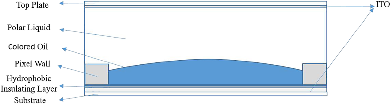
FIGURE 1. Pixel structure of an EWD panel. The structure includes a top plate, ITO, fluid (colored oil and polar liquid), pixel wall, hydrophobic insulating layer, and substrate. The pixel wall is hydrophilic, and the hydrophobic insulating layer is hydrophobic and lipophilic.

At present, there are still some defects in EWDs, such as oil-splitting, charge trapping, oil overflow, and so on [10]. To solve these defects and further improve the display performance of EWDs, many researchers have made many attempts. For example, a three-dimensional EWD model was established and the process of fluid flow was simulated. In the simulation, the principle of phase-field was used to simulate the movement of oil interface successfully, and the influence of contact angle of the pixel wall on oil-splitting was studied [16]. However, the problem of oil-splitting caused by high voltage had not been solved. For oil-splitting, the influence of surface tension and contact angle in the fluid was considered. Through model simulation and numerical analysis, the influence of contact angle and surface tension on oil-splitting was proved [17]. In addition, the oil-splitting was affected by the oil thickness. The oil in the EWDs pixel was non-uniform, and the oil was split at the thinnest point [18]. However, the influence of thickness change on the process of oil movement was not considered. To suppress the oil-splitting, a driving waveform which consisted of four stages: starting, rising, displaying, and recovering was proposed. Starting from a low voltage to drive the oil can suppress oil-splitting effectively [19]. However, the speed of oil movement was slowed down.

In order to suppress the oil-splitting, a simulation model was established by COMSOL Multiphysics software. The relationship between electrostatic field force and oil shape change was studied by this model. And then, the change characteristic of oil shape was obtained in a switch-on process. According to this characteristic, a driving waveform which can suppress the oil-splitting effectively was proposed.

Numerical Methodology

The simulation of EWDs was implemented by establishing and calculating numerical equations. It was done to track the change of the oil-water interface in the model [20]. By using COMSOL Multiphysics software and Finite-Element method to simulate Two-Phase laminar flow with the electrostatic field, the physical field of laminar flow was coupled with the phase-field and the electrostatic field [21]. The finite element analysis method can be used to solve numerical calculation problems including the Cahn-Hilliard equation, Laplace equation, and Navier-Stokes equation [22]. Meanwhile, to solve Maxwell’s stress tensor equation, an electrostatic field module was added to the simulation. The electrostatic field force of the electrostatic field module was fed back into the laminar flow module. The Navier-Stokes equation and phase-field equation were solved according to specified boundary conditions and calculation results of electrostatic field.

Governing Equations

Phase-field is used to describe the dynamic process of a two-phase flow interface. The movement of interface is tracked indirectly by solving two equations. One of them is used to solve phase-field variable $\varnothing$ and the other is used to solve the mixed energy density $\text{ψ}$ [16, 23, 24]. The position of the interface is determined by minimum free energy [23]. A large number of data have been proved that the phase-field method could effectively predict droplet movement on the solid surface [25, 26]. Eqs. 1–3 represent the governing equation of phase-field [27]. Eq. 4 describes the relationship between $\gamma$ and $\epsilon$.

$\frac{\partial \varnothing }{\partial t}+u\cdot \nabla \varnothing =\nabla \cdot \frac{\gamma \lambda }{{\epsilon }^2}\nabla \psi (1)$

$\psi =-\nabla \cdot {\epsilon }^2\nabla \varnothing +\left({\varnothing }^2-1\right)\varnothing +\left(\frac{{\epsilon }^2}{\lambda }\right)\frac{\partial f_{ext}}{\partial \varnothing }(2)$

$\sigma =\frac{2\sqrt{2}}{3}\frac{\lambda }{\epsilon }(3)$

$\gamma =\chi {\epsilon }^2(4)$

Where $\text{λ}$ is the energy density and $\text{ε}$ is the capillary width. Eq. 3 describes the relationship between these two parameters and the surface tension coefficient $\text{σ}$. The $\gamma$ is the mobility parameter and $\chi$ is the mobility tuning parameter in Eq. 4. $\varnothing$ was set to 1 for oil and −1 for water. In order to couple the electrostatic field with the laminar flow field, the dielectric constant, density, and viscosity between diffusion interfaces need to be calculated by Eqs. 5–7.

$\rho ={\rho }_1+\left({\rho }_2-{\rho }_1\right)\varnothing (5)$

$\mu ={\mu }_1+\left({\mu }_2-{\mu }_1\right)\varnothing (6)$

${\epsilon }_r={\epsilon }_{r1}+\left({\epsilon }_{r2}-{\epsilon }_{r1}\right)\varnothing (7)$

Where $\text{ρ}$, $\text{μ}$, and ${\text{ε}}_r$ represent the density, viscosity, and dielectric constant of fluids, respectively. The mean curvature between the two liquids interfaces was calculated by Eqs. 8,9 [27].

$\kappa =2\left(1+\varnothing \right)\left(1-\varnothing \right)\frac{G}{\sigma }(8)$

$G=\lambda \left(-{\nabla }^2\varnothing +\frac{\varnothing \left({\varnothing }^2-1\right)}{{\epsilon }^2}\right)+\frac{\partial f}{\partial \varnothing }(9)$

Where $\text{κ}$ and $\text{G}$ represent the mean curvature and the chemical potential, respectively.

The laminar flow field can be solved by the Navier-Stokes equation and continuity equation [28]. The Navier-Stokes equation is described as Eq. 10. To depict the movement of two immiscible liquids, the transport of mass and momentum are governed by incompressible Navier–Stokes equations.

$\rho \left(\frac{\partial u}{\partial t}+u\cdot \nabla u\right)=-\nabla p+\nabla \cdot \left(\mu \left(\nabla u+{\left(\nabla u\right)}^T\right)-\frac{2}{3}u\left(\nabla \cdot u\right)I\right)+F(10)$

$F=F_{st}+\rho g+F_{vf}(11)$

Where $u$, $p$, $\rho$, and $\mu$ represent the velocity, pressure, density, and dynamic viscosity of the fluid respectively. Each term in Eq. 10 corresponds to the inertial force, pressure, viscous force, and external force, respectively. The external force consists of surface tension, gravity, and a volume force, the $F_{st}$, $g$ and $F_{vf}$ represent the surface tension, gravity acceleration, and volume force, respectively.

As stated in Eqs. 10,11, the coupling between the laminar flow field and the electrostatic field is achieved by applying the electrostatic volume force to the Navier-Stokes equation. The electrostatic field force is the main factor that can cause fluid-flowing [16]. In addition, the electrostatic field force can be obtained by calculating the divergence based on Maxwell Stress Tensor (MST) [16], and the calculation is expressed in Eq. 12.

$F_{vf}=\nabla T_{ik}(12)$

MST formula is described by Eq. 13.

$T=E{D}^T-\frac{1}{2}\left(D\cdot EI\right)(13)$

Where $I$ is the identity matrix, $E$ is the electric field and $D$ is the electric displacement field, and their relationship is described by Eqs. 14,15.

$E=-\nabla V(14)$

$D={\epsilon }_0{\epsilon }_{r}E(15)$

In a two-dimensional model simulation, the MST is expressed as Eq. 16.

$T=\left[\begin{array}{cc}{T}_{xx}& T_{xy}\\ T_{yx}& T_{yy}\end{array}\right](16)$

Eq. 17 can be obtained by substituting parameters.

$T=\left[\begin{array}{cc}{\epsilon }_0{\epsilon }_r{E}_x^2-\frac{1}{2}{\epsilon }_0{\epsilon }_r\left(E_x^2+E_y^2\right)& {\epsilon }_0{\epsilon }_r{E}_x{E}_y\\ {\epsilon }_0{\epsilon }_r{E}_x{E}_y& {\epsilon }_0{\epsilon }_r{E}_y^2-\frac{1}{2}{\epsilon }_0{\epsilon }_r\left(E_x^2+E_y^2\right)\end{array}\right](17)$

Where $E_x$ and $E_y$ represent the horizontal and vertical electric fields respectively. The variation of volume force caused by the electrostatic field acts on the interface between oil and water, and the calculation can be expressed in Eq. 18.

$F=\left[\begin{array}{cc}\frac{\partial \left(T_{xx}\right)}{\partial x}& \frac{\partial \left(T_{xy}\right)}{\partial y}\\ \frac{\partial \left(T_{yx}\right)}{\partial x}& \frac{\partial \left(T_{yy}\right)}{\partial y}\end{array}\right](18)$

When an electric field is applied, the water is in contact with the hydrophobic insulation layer with the action of electrostatic field force [29, 30], the electrostatic field force can be described by Eq. 19.

$F_e=\frac{1}{2}{d}_{hyd}{\epsilon }_0{\epsilon }_{hyd}{E}_{hyd}^2(19)$

Where $d_{hyd}$, ${\epsilon }_{hyd}$ and $E_{hyd}$ represent the thickness of the hydrophobic insulation layer, dielectric constant, and electric field strength on the hydrophobic insulation layer, respectively. Therefore, the force balance on the contact line can be derived from the Lippmann-Young equation, as shown in Eq. 20.

$\cos {\theta }_e=\cos {\theta }_{hyd}+\frac{{\epsilon }_0{\epsilon }_{hyd}{V}^2}{2d_{hyd}{\gamma }_{ow}}(20)$

Where ${\theta }_e$, ${\theta }_{hyd}$, and ${\gamma }_{ow}$ are the EW contact angle, Young’s contact angle of the hydrophobic dielectric layer, and the surface tension, respectively.

Boundary Conditions

In the simulation model, boundary conditions are the prerequisites for determining the solution of governing equations on the boundary. The zero-charge boundary condition should be set on all sides of the model. For electrostatic field boundary conditions, the voltage V and the ground need to be specified. The wetted wall, the initial interface, and the outlet need to be specified in phase-field boundary conditions. The wetted wall boundary can be calculated by Eqs. 21,22.

$n\cdot {\epsilon }^2\nabla \varnothing ={\epsilon }^2\cos \left({\theta }_w\right)\left|\nabla \varnothing \right|(21)$

$n\cdot \frac{\gamma \lambda }{{\epsilon }^2}\nabla \psi =0(22)$

The interface of the two-phase flow was selected as an initial boundary condition. Both sides of the model (except the pixel walls) were selected as inlet and outlet boundary conditions. In addition, initial values of pressure and velocity in the laminar flow field were set to 0. The wall condition was set to no slip. These setting of boundary conditions were shown in Figure 2. The dotted box in Figure 2 represents the symmetric boundary condition.

FIGURE 2

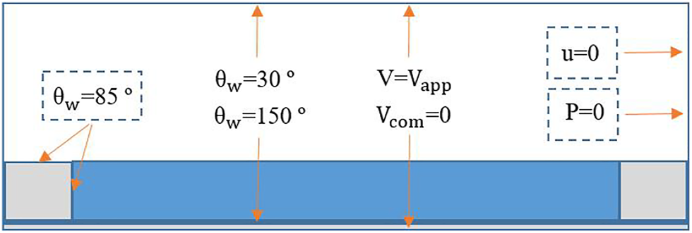
FIGURE 2. The boundary conditions for the electrostatic field, phase field, and laminar flow field. Where $\text{u}$, $\text{P}$, ${\theta }_w$, and $\text{V}$ represents the velocity, pressure, contact angle, and voltage of the boundary conditions respectively. The pixel wall and outlet are symmetrical boundary conditions.

Process and Discussion

The parameters used in the simulation were shown in Table 1. The fluid (oil and water) in the model was set to incompressible flow. It was assumed that the temperature (25°C) was kept constant during the fluid movement, so the thermal expansion of the fluid was ignored. The influence of pressure on dynamic viscosity was ignored. In addition, the Bond number describes the relationship between gravity and surface tension in the EWDs model, and it is far less than 1. So the gravity can be neglected [16]. In the simulation, the polar liquids were replaced by water [31].

TABLE 1

TABLE 1. Structure, material, and interface parameters of the model.

The proposed simulation model was shown in Figure 2. The natural spreading and shrinking process of oil were realized in this model. To describe the display performance of EWDs, it is necessary to calculate the aperture ratio. The aperture ratio is an important performance index of EWDs, which is a proportion of opening area in a whole pixel [20]. When the aperture ratio was calculated in two dimensions, the bottom of the EWD was considered as a square, and $A_r$ is used to represent the aperture ratio, $L$ is the length of the contact line between the oil and the hydrophobic insulating layer in two dimensions structure, and $d$ is the area of the hydrophobic insulating layer. The aperture ratio was calculated by using Eq. 23.

$A_r=\frac{4\times d^2-\pi L^2}{4\times d^2}\times 100\%(23)$

When the electric field inside a pixel was analyzed, the electric field formula was used, as shown in Eq. 24. Where $E$, $U$, $d$ represents the electric field, the voltage, and the distance between the two potentials, respectively.

$E=\frac{U}{d}(24)$

In this paper, the EWD model was implemented by COMSOL Multiphysics 5.4. The aperture ratio test platform was shown in Figure 3. This test platform included a waveform editing system, a signal amplifier, and a detection system. The waveform editing system was used to edit and generate waveform signals, which was consisted of a computer and a function signal generator. The signal was amplified by the signal amplifier to drive the oil. The detection system was used to collect oil movement image of EWD panel in real time, which was consisted of a high-speed camera and an image processing system. The aperture ratio was obtained by the image processing platform.

FIGURE 3

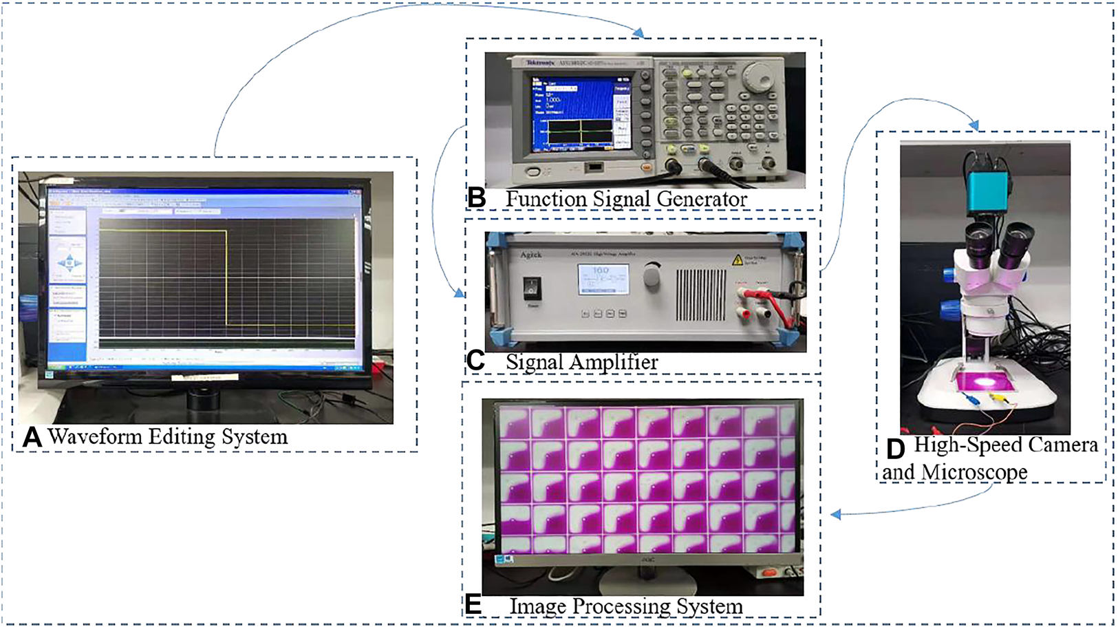
FIGURE 3. An aperture ratio test platform for EWDs (A) A waveform editing system (B) A function signal generator (C) A signal amplifier (D) A high-speed camera and a microscope (E) An image processing system.

Influence of Dynamic Viscosity

The dynamic viscosity is an important parameter in fluid. The dynamic viscosity of oil can affect the aperture ratio and response time [20]. The response time is expressed as T. In one driving cycle, the time for applying the driving waveform is represented by T1, and the time when the pixel reaches the maximum aperture ratio is represented by T2. The response time is equal to the difference between T2 and T1. In this paper, an experiment of oil dynamic viscosity from 0.0005 Pa·s to 0.003 Pa·s with an interval of 0.0005 Pa·s was designed, and the experimental results were shown in Figure 4. When the dynamic viscosity was changed from 0.002 Pa·s to 0.003 Pa·s, the response time was shorter and the aperture ratio was larger. Figure 5 showed that when the dynamic viscosity of oil was less than 0.0015 Pa·s, the oil was split into two pieces. Otherwise, the oil was pushed into a corner with a whole block. Therefore, the oil with a dynamic viscosity from 0.002 Pa·s to 0.003 Pa·s should be selected in current conditions. Figure 6 showed the process of a switch-on and a switch-off in a pixel with specific conditions. The conditions were that the voltage was 32 V and the oil dynamic viscosity was 0.002 Pa·s. The results showed that the oil was pushed into a corner with a whole block. So, the dynamic viscosity of oil was set to 0.002 Pa·s.

FIGURE 4

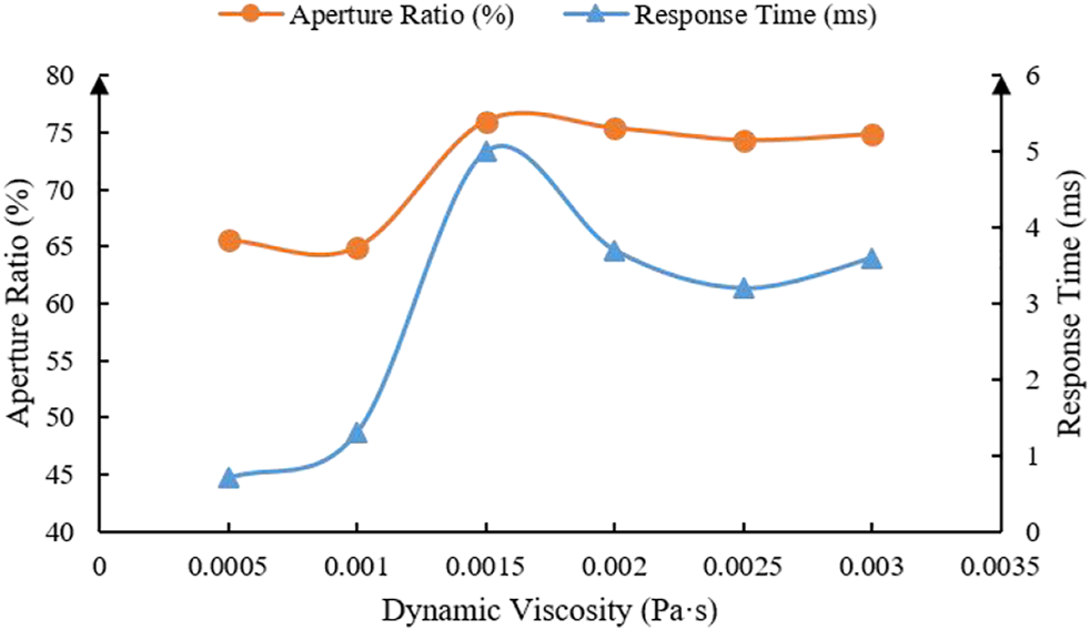
FIGURE 4. The influence of oil dynamic viscosity on pixel aperture ratio and response time.

FIGURE 5

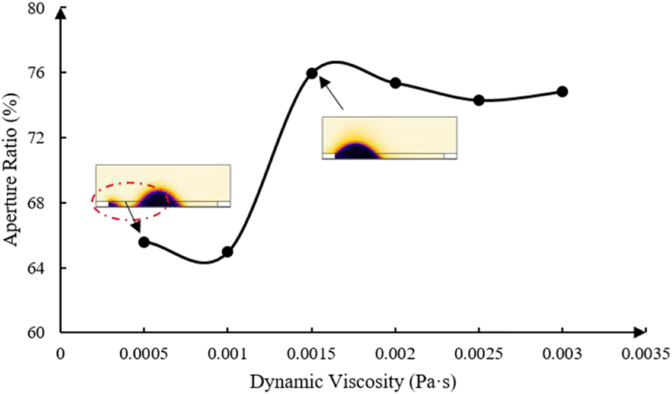
FIGURE 5. The influence of oil with different dynamic viscosity on oil-splitting. When the dynamic viscosity of the oil was higher than 0.0015 Pa·s, the oil was pushed with a whole block. Otherwise, the oil was divided into two pieces.

FIGURE 6

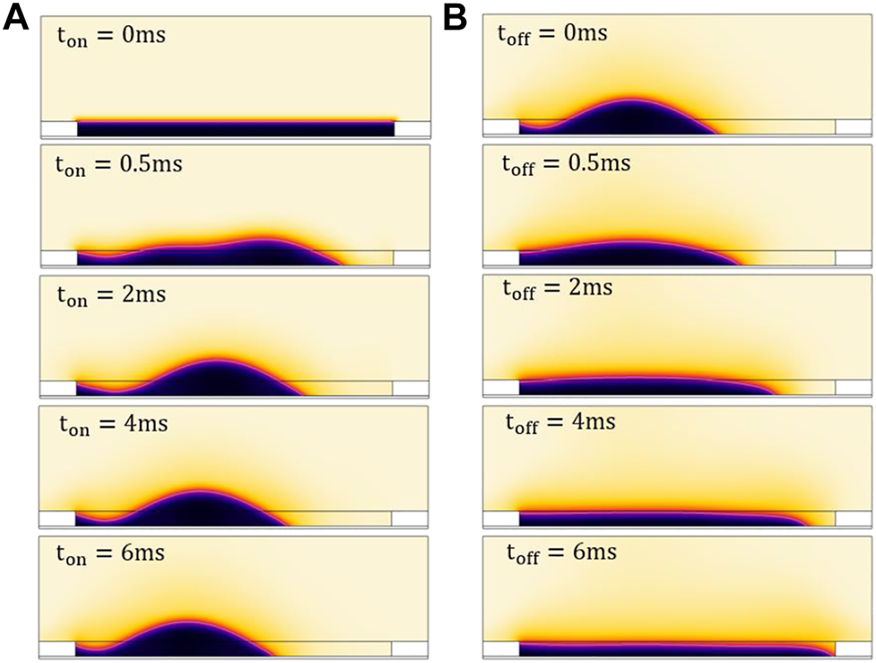
FIGURE 6. In COMSOL software, the movement process of oil and water (black represents oil, light yellow represents water) was intercepted (A) After applying 32 V voltage, the oil was shrunk with the action of electrostatic field force, which was completed in 4 ms. (B) When the driving voltage was removed, the oil was naturally spread, and the process was completed in 6 ms.

Influence of Driving Waveforms

In a pixel, the voltage of driving waveform was converted into electrostatic field force and applied to the water and oil. In the simulation, the gradually increasing voltage was set by the parametric scanning method, and the results were shown in Figure 7. When the voltage was lower than 16 V, the shape of oil was squeezed down at both sides of a pixel, but the oil was not split. When the voltage was changed from 16 to 36 V, the aperture ratio was almost increased linearly. When the voltage was higher than 36 V, the aperture ratio was increased slowly and reached the maximum. At the same time, the oil was split into two pieces. The blue curve in Figure 7 represented the maximum aperture ratio of an actual EWD pixel when the voltage was changed from 16 to 36 V. The length and width of an actual pixel were 150 and 150 μm, respectively. The aperture ratio of the actual pixel was measured on the test platform in Figure 3. The results showed that the value of simulation was close to the actual before 20 V. In the range of 20–28 V, the simulation value was 4.3% higher than the actual, and in the range of 28–36 V, the simulation value was 10.5% higher than the actual. Altogether, the trends between these two were consistent. Therefore, the accuracy of this simulation model was verified.

FIGURE 7

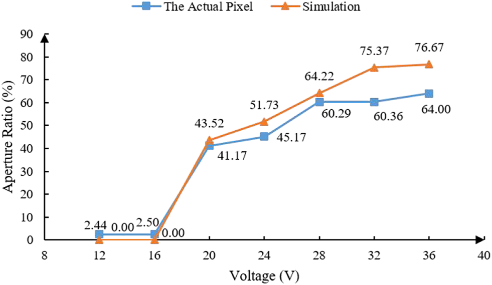
FIGURE 7. The aperture ratio between simulation and an actual pixel. When the voltage was changed from 16 to 36 V, the change curve of aperture ratio between the actual pixel and simulation was obtained. The length and width of an actual pixel were 150 and 150 μm respectively. The changing trend of aperture ratio was consistent between simulation and actual EWD pixel.

The driving waveform has influence on the movement of oil [32–34]. To comprehend the acceleration ability of oil with the action of driving waveforms in one cycle, these driving waveforms with a different rising slope were designed, as shown in Figure 8. The change of aperture ratio with the action of four driving waveforms was shown in Figure 9. With the slope increased, the response time was shorter. When the slope was infinite (square waveform), the oil was split into two pieces. The experimental data showed that the moment when the pixel reached the maximum aperture ratio later than the moment that the driving waveform reached the maximum voltage for 2–5 ms. The greater the slope, the stronger the oil acceleration. So, a maintenance period of 2–5 ms should be set to drive a pixel for reaching the maximum aperture ratio. It took more than 6 ms in the natural spreading stage.

FIGURE 8

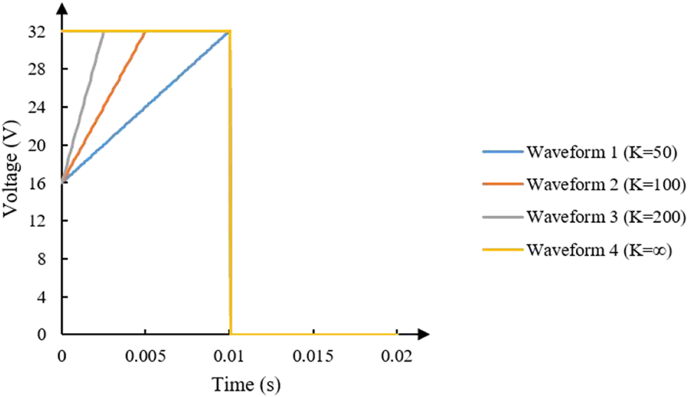
FIGURE 8. Four driving waveforms with different slopes were designed. The starting voltage was set to 16 V. K in the cleft was the slope, and the slopes of the four waveforms are 50, 100, 200, and infinite, respectively. The effective driving cycle was 10 ms, and the latter 10 ms was set to 0 V.

FIGURE 9

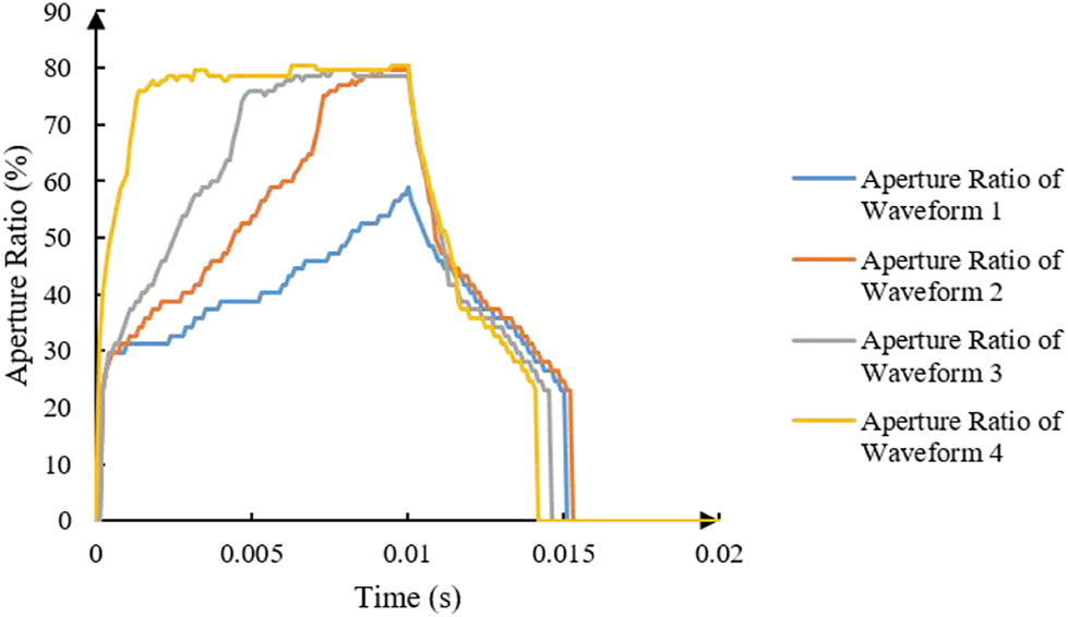
FIGURE 9. The pixel aperture ratio was obtained with four driving waveforms.

Relationship Between Electrostatic Field Force and Oil Movement

The forces on the fluid can be divided into volume force and external force. The volume force can be divided into surface tension and electrostatic field force. The electrostatic field force is a key factor that affects the oil movement of EWDs [35, 36]. To obtain the relationship between the movement status of oil with a whole block and the internal electrostatic field force. Parameters were determined based on Waveform 2 in Figure 8, the voltage was set to 32 V and the oil dynamic viscosity was 0.002 Pa·s.

The change of the internal electric field inside a pixel was shown in Figure 10. In the vertical direction, the internal space of the pixel was divided into a water channel and an oil-water mixed channel. As shown in Figure 10B, the internal space of the pixel can be divided into areas 1, 2, 3, and 4, respectively, areas 1, 3 were oil-water mixed channels, and areas 2, 4 were water channels. E1, E2, E3, and E4 represented the internal electric fields formed by areas 1, 2, 3, and 4, respectively. In the analysis process, the water with a high dielectric constant (80) as a conductor of electricity and oil as an insulator was considered. According to Eq. 24, the internal voltage U was 0 V in the water channel, so the internal electric field E was 0 (V/m). In the area of the oil-water mixed channel, if U remained unchanged and d was increased, the internal electric field was decreased. On the contrary, the internal electric field was increased. Therefore, the internal electric field force was proportional to the thickness of the oil, and the oil was split easier in the thin area. The red arrows in Figure 10B indicated the direction of the internal electric field. When the water was considered as a conductor of electricity, the voltage at the oil-water interface was the same. As the height of the oil increased, the electric field at the high of the oil was smaller, and the electric field at both sides was greater than the highest. Therefore, a non-uniform electric field was formed in the oil, and the oil formed a spherical cap shape with the action of the non-uniform internal electrostatic field.

FIGURE 10

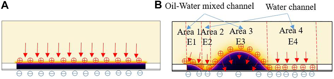
FIGURE 10. The change of the internal electric field inside of a pixel (A) The internal electric field of the initial interface (B) The internal electric field in the process of oil movement. E1, E2, E3, and E4 represented the internal electric fields formed by areas 1, 2, 3, and 4, respectively.

The change of the internal electrostatic field force inside a pixel was shown in Figure 11. The result was obtained by the integral calculation of electrostatic field forces in a pixel space (except the pixel walls). When the oil was in State 1, a new water channel was formed in the oil ruptured area, and the internal electric field was reduced in this area. So, the electrostatic field force was reduced at this stage. Then, the voltage was increased linearly, the electric field in the pixel space was increased overall. As a result, the electrostatic field force was also increased. When the oil became State 2, the oil was pushed to the highest. Although the voltage kept the maximum, the internal electrostatic field force was reduced. This was mainly due to the larger water channel area.

FIGURE 11

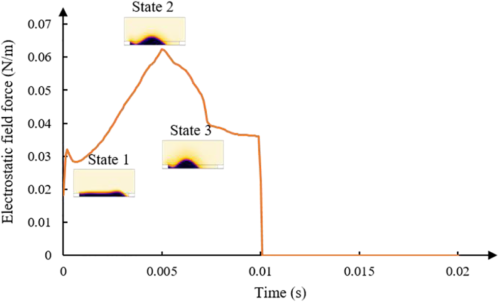
FIGURE 11. The relationship between fluid status and electrostatic field force. Taking Waveform 2 as the input term, the electrostatic field force in a pixel space was integrated, and the results of the electrostatic field force in the driving period were obtained.

Driving Waveform Design for Suppressing Oil-Splitting

In a two-dimensional EWD model simulation, a pixel switch-on process can be divided into three stages. In the first stage, oil was ruptured randomly on one side of a pixel. The other side was squeezed down, but not ruptured. This stage was maintained about 1 ms. In the second stage, oil was continuously squeezed, the oil was driven both vertically and horizontally with the action of the non-uniform electrostatic field force. If the voltage was large enough, oil on the side which was not ruptured previously was split. This stage was maintained about 2–5 ms. In the third stage, oil was driven horizontally, and the height of oil was almost unchanged. By analyzing these stages, the conclusions were obtained as follows. The oil was thin and the electrostatic field force applied to the oil was large in the first stage. When a high voltage more than 36 V was applied, the oil was split into two pieces. The oil-splitting appeared in the first and second stages. So, combined with the analysis of oil movement in the first and second stages, a driving waveform was proposed for suppressing the oil-splitting. The proposed driving waveform was divided into three stages as shown in Figure 12. In the first stage, the waveform started at 36 V (high voltage), then was dropped to 30 V rapidly, and maintained for 0.5 ms, respectively. The purpose of this stage was mainly to drive the oil to rupture on one side. In stage 2, the voltage value was maintained at 30 V for 2.5 ms. At this stage, oil was mainly driven in one direction horizontally. In stage 3, when the oil was pushed thick enough, the voltage can be increased, and the oil was not split anymore. This stage was to improve the response speed of the pixel. When the square waveform was applied to this model, the oil was split into two pieces at 1.5 ms as shown in Figure 13A, and then the oil was driven to the middle of a pixel at 5 ms. When the proposed driving waveform was applied to this model, the oil was pushed a corner with a whole block as shown in Figure 13B. The result showed that the proposed driving waveform can effectively suppress oil-splitting, and the aperture ratio was increased by 2.9% compared to the square waveform.

FIGURE 12

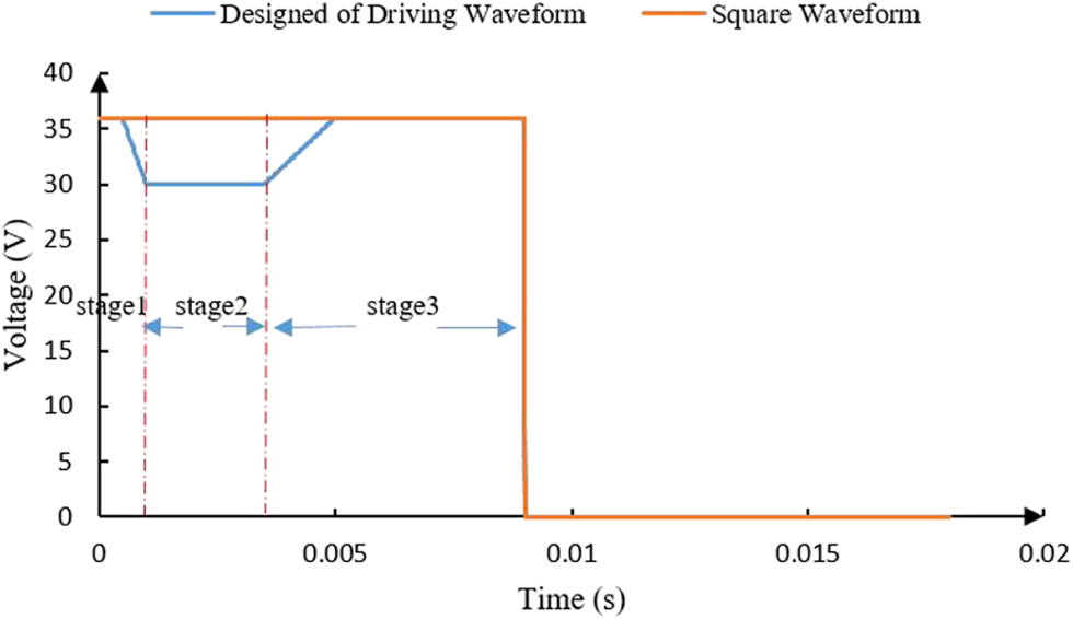
FIGURE 12. The proposed driving waveform and the traditional square waveform. The proposed driving waveform had three stages which were maintained for 1 ms, 2.5 ms, and 5.5 ms, respectively, and the period of the square waveform and the proposed driving waveform were both 18 ms. The rest of the blue curve overlapped with the square waveform.

FIGURE 13

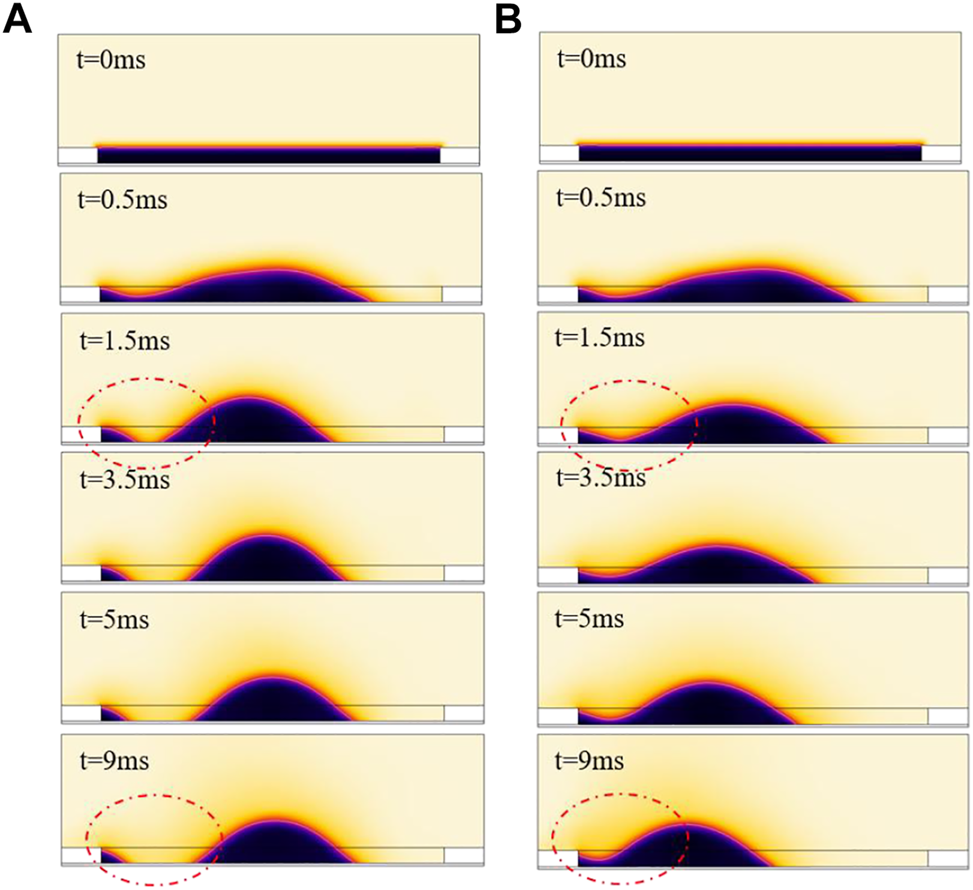
FIGURE 13. When the proposed driving waveform and the square waveform were applied, the change of oil status was obtained (A) With the driving of the square waveform, the oil was split into two pieces, the aperture ratio was 76.67% (B) With the driving of the proposed driving waveform, the oil was pushed into a corner with a whole block, and the aperture ratio was 78.89%.

Conclusion

In this paper, a two-dimensional EWD model was established. This model was used to simulate the influence of dynamic viscosity, voltage, and waveform on oil-splitting. The oil was easily broken into two pieces with a high voltage. In addition, the internal electrostatic field force and oil movement were affected by each other. On the basis of the traditional square waveform, the proposed narrow falling ramp drove the oil to rupture quickly on one side of a pixel. The proposed low voltage maintenance stage can effectively suppress the oil-splitting. After applying this optimized waveform, the aperture ratio of a pixel was increased. The simulation model can provide a prediction scheme for the selection of oil and the design of the driving system in practical application. By adjusting part of the structure or material parameters of the model, it can be applied to other schemes of EWDs.

Data Availability Statement

The raw data supporting the conclusions of this article will be made available by the authors, without undue reservation.

Author Contributions

SL, HS, and QZ: investigation, methodology, formal analysis, editing.SL: writing – review, and editing. All authors contributed to the article and approved the submitted version.

Funding

Supported by the National Key Research and Development Program of China (2016YFB0401501), Program for Guangdong Innovative and Enterpreneurial Teams (No. 2019BT02C241), Science and Technology Program of Guangzhou (No. 2019050001), Program for Chang Jiang Scholars and Innovative Research Teams in Universities (No. IRT_17R40), Guangdong Provincial Key Laboratory of Optical Information Materials and Technology (No. 2017B030301007), Guangzhou Key Laboratory of Electronic Paper Displays Materials and Devices (201705030007), and the 111 Project.

Conflict of Interest

The authors declare that the research was conducted in the absence of any commercial or financial relationships that could be construed as a potential conflict of interest.

References

1. Jones TB. An Electromechanical Interpretation of Electrowetting. J Micromech Microeng (2005) 15(6):1184–7. doi:10.1088/0960-1317/15/6/008

CrossRef Full Text | Google Scholar

2. Beni G., Hackwood S.. Electro-wetting Displays. Appl Phys Lett (1981) 38(4):207–9. doi:10.1063/1.92322

CrossRef Full Text | Google Scholar

3. Bai PF., Hayes RA., Jin M., Shui L., Yi ZC., Wang L., et al. Review of Paper-Like Display Technologies (Invited Review). Pier (2014) 147:95–116. doi:10.2528/PIER13120405

CrossRef Full Text | Google Scholar

4. Yi Z., Feng H., Zhou X., Shui L. Design of an Open Electrowetting on Dielectric Device Based on Printed Circuit Board by Using a Parafilm M. Front Phys (2020) 8:193. doi:10.3389/fphy.2020.00193

CrossRef Full Text | Google Scholar

5. Feng H., Yi Z., Yang R., Qin X., Shen S., Zeng W., et al. Designing Splicing Digital Microfluidics Chips Based on Polytetrafluoroethylene Membrane. Micromachines (2020) 11(12):1067. doi:10.3390/mi11121067

PubMed Abstract | CrossRef Full Text | Google Scholar

6. Wang L., Yi Z., Jin M., Shui L., Zhou G. Improvement of Video Playback Performance of Electrophoretic Displays by Optimized Waveforms with Shortened Refresh Time. Displays (2017) 49:95–100. doi:10.1016/j.displa.2017.07.007

CrossRef Full Text | Google Scholar

7. Shen S., Gong Y., Jin M., Yan Z., Xu C., Yi Z., et al. Improving Electrophoretic Particle Motion Control in Electrophoretic Displays by Eliminating the Fringing Effect via Driving Waveform Design. Micromachines (2018) 9(4):143. doi:10.3390/mi9040143

PubMed Abstract | CrossRef Full Text | Google Scholar

8. Li JS., Tang Y., Li ZT., Li JX., Ding XR., Yu BH., et al. Toward 200 Lumens Per Watt of Quantum-Dot White-Light-Emitting Diodes by Reducing Reabsorption Loss. ACS Nano (2021) 15(1):550–62. doi:10.1021/acsnano.0c05735

PubMed Abstract | CrossRef Full Text | Google Scholar

9. Li Z., Cao K., Cao K., Li J., Tang Y., Ding X., et al. Review of Blue Perovskite Light Emitting Diodes with Optimization Strategies for Perovskite Film and Device Structure. Opto-Electronic Adv (2021) 4(2):20001901–15. doi:10.29026/oea.2021.200019

CrossRef Full Text | Google Scholar

10. Li W., Wang L., Zhang T., Lai S., Liu L., He W., et al. Driving Waveform Design with Rising Gradient and Sawtooth Wave of Electrowetting Displays for Ultra-low Power Consumption. Micromachines (2020) 11(2):145. doi:10.3390/mi11020145

PubMed Abstract | CrossRef Full Text | Google Scholar

11. Yi Z., Huang Z., Lai S., He W., Wang L., Chi F., et al. Driving Waveform Design of Electrowetting Displays Based on an Exponential Function for a Stable Grayscale and a Short Driving Time. Micromac (2020) 11(3):313. doi:10.3390/mi11030313

PubMed Abstract | CrossRef Full Text | Google Scholar

12. Jin M., Shen S., Yi Z., Zhou G., Shui L. Optofluid-Based Reflective Displays. Micromac (2018) 9(4):159. doi:10.3390/mi9040159

PubMed Abstract | CrossRef Full Text | Google Scholar

13. Yi Z., Shui L., Wang L., Jin M., Hayes RA., Zhou G. A Novel Driver for Active Matrix Electrowetting Displays. Displ (2015) 37:86–93. doi:10.1016/j.displa.2014.09.004

CrossRef Full Text | Google Scholar

14. Yi Z., Liu L., Wang L., Li W., Shui L., Zhou G. A Driving System for Fast and Precise Gray-Scale Response Based on Amplitude-Frequency Mixed Modulation in TFT Electrowetting Displays. Micromac (2019) 10(11):732. doi:10.3390/mi10110732

PubMed Abstract | CrossRef Full Text | Google Scholar

15. Liu L., Bai P., Yi Z., Zhou G. A Separated Reset Waveform Design for Suppressing Oil Backflow in Active Matrix Electrowetting Displays. Micromac (2021) 12(5):491. doi:10.3390/mi12050491

CrossRef Full Text | Google Scholar

16. Hsieh WL., Lin CH., Lo KL., Lee KC., Cheng WY., Chen KC. 3D Electrohydrodynamic Simulation of Electrowetting Displays. J Micromech Microeng (2014) 24(12):125024. doi:10.1088/0960-1317/24/12/125024

CrossRef Full Text | Google Scholar

17. Walker S. W., Shapiro B. Modeling the Fluid Dynamics of Electrowetting on Dielectric (EWOD). J Microelectromech Syst (2006) 15(4):986–1000. doi:10.1109/JMEMS.2006.878876

CrossRef Full Text | Google Scholar

18. Zhou M., Zhao Q., Tang B., Groenewold J., Hayes RA., Zhou G. Simplified Dynamical Model for Optical Response of Electrofluidic Displays. Displ (2017) 49:26–34. doi:10.1016/j.displa.2017.05.003

CrossRef Full Text | Google Scholar

19. Luo Z., Fan J., Xu J., Zhou G., Liu S. A Novel Driving Scheme for Oil-Splitting Suppression in Electrowetting Display. Opt Rev (2020) 27(4):339–45. doi:10.1007/s10043-020-00601-z

CrossRef Full Text | Google Scholar

20. Roques-Carmes T., Hayes RA., Schlangen LJM. A Physical Model Describing the Electro-Optic Behavior of Switchable Optical Elements Based on Electrowetting. J Appl Phys (2004) 96(11):6267–71. doi:10.1063/1.1810192

CrossRef Full Text | Google Scholar

21. Yang G., Zhuang L., Bai P., Tang B., Henzen A., Zhou G. Modeling of Oil/Water Interfacial Dynamics in Three-Dimensional Bistable Electrowetting Display Pixels. ACS Omega (2020) 5(10):5326–33. doi:10.1021/acsomega.9b04352

PubMed Abstract | CrossRef Full Text | Google Scholar

22. Kim J.. Phase-Field Models for Multi-Component Fluid Flows. Commun Comput Phys (2012) 12(3):613–61. doi:10.4208/cicp.301110.040811a

CrossRef Full Text | Google Scholar

23. Zhao Q., Tang B., Dong B., Li H., Zhou R., Guo Y., et al. Electrowetting on Dielectric: Experimental and Model Study of Oil Conductivity on Rupture Voltage. J Phys D: Appl Phys (2018) 51(19):195102. doi:10.1088/1361-6463/aabb69

CrossRef Full Text | Google Scholar

24. Yue P., Feng JJ., Liu C., Shen J. A Diffuse-Interface Method for Simulating Two-phase Flows of Complex Fluids. J Fluid Mech (2004) 515:293–317. doi:10.1017/S0022112004000370

CrossRef Full Text | Google Scholar

25. Yurkiv V., Yarin AL., Mashayek F. Modeling of Droplet Impact onto Polarized and Nonpolarized Dielectric Surfaces. Langmuir (2018) 34(34):10169–80. doi:10.1021/acs.langmuir.8b01443

PubMed Abstract | CrossRef Full Text | Google Scholar

26. Zhu G., Yao J., Zhang L., Sun H., Li A., Shams B. Investigation of the Dynamic Contact Angle Using a Direct Numerical Simulation Method. Langmuir (2016) 32(45):11736–44. doi:10.1021/acs.langmuir.6b02543

PubMed Abstract | CrossRef Full Text | Google Scholar

27. Cahn JW., Hilliard JE.. Free Energy of a Nonuniform System. I. Interfacial Free Energy. J Chem Phys (1958) 28(2):258–67. doi:10.1063/1.1744102

CrossRef Full Text | Google Scholar

28. Dolatabadi A., Arzpeyma A., Wood-Adams P., Bhaseen S. A Coupled Electro-Hydrodynamic Numerical Modeling of Droplet Actuation by Electrowetting. Colloids Surfa, A Physicoche Eng Aspects (2008) 323(1/3):28–35. doi:10.1016/j.colsurfa.2007.12.025

CrossRef Full Text | Google Scholar

29. Jones TB., Gunji M., Washizu M., Feldman MJ. Dielectrophoretic Liquid Actuation and Nanodroplet Formation. J Appl Phys (2001) 89(2):1441–8. doi:10.1063/1.1332799

CrossRef Full Text | Google Scholar

30. Jones TB., Fowler JD., Chang YS., Kim CJ. Frequency-based Relationship of Electrowetting and Dielectrophoretic Liquid Microactuation. Langmuir (2003) 19(18):7646–51. doi:10.1021/la0347511

CrossRef Full Text | Google Scholar

31. Jones TB. On the Relationship of Dielectrophoresis and Electrowetting. Langmuir (2002) 18(11):4437–43. doi:10.1021/la025616b

CrossRef Full Text | Google Scholar

32. Yi Z., Feng W., Wang L., Liu L., Lin Y., He W., et al. Aperture Ratio Improvement by Optimizing the Voltage Slope and Reverse Pulse in the Driving Waveform for Electrowetting Displays. Micromachines (2019) 10(12):862. doi:10.3390/m11012086210.3390/mi10120862

PubMed Abstract | CrossRef Full Text | Google Scholar

33. Feng HQ., Yi ZC., Sun ZZ., Zeng WJ., Wang L., Yang JJ., et al. A Spliceable Driving System Design for Digital Microfluidics Platform Based on Indium Tin Oxide Substrate. J Nanoelectronics Optoelectronics (2020) 15(9):1127–36. doi:10.1166/jno.2020.2838

CrossRef Full Text | Google Scholar

34. Zeng W., Yi Z., Zhao Y., Zeng W., Ma S., Zhou X., et al. Design of Driving Waveform Based on Overdriving Voltage for Shortening Response Time in Electrowetting Displays. Front Phys (2021) 9:642682. doi:10.3389/fphy.2021.642682

CrossRef Full Text | Google Scholar

35. Kang KH. How Electrostatic fields Change Contact Angle in Electrowetting. Langmuir (2002) 18(26):10318–22. doi:10.1021/la0263615

CrossRef Full Text | Google Scholar

36. Brabcova Z., McHale G., Wells GG., Brown CV., Newton MI. Electric Field Induced Reversible Spreading of Droplets into Films on Lubricant Impregnated Surfaces. Appl Phys Lett (2017) 110(12):121603. doi:10.1063/1.4978859

CrossRef Full Text | Google Scholar