Modeling geomagnetic induction in submarine cables

1 Introduction

Submarine cables have become a vital component of our modern infrastructure. They carry more than 95% of international internet traffic [1], so any disruption to their operation can have wide-ranging consequences across the globe. Although studies focused on natural hazards that may damage cables such as submarine landslides and tsunamis have increased [1], the possibility of space weather effects has generally not been considered in such studies. Over the last 20 years - the lifetime of modern cable systems - space weather activity has been low; but more extreme space weather events have occurred in the past and it is uncertain how modern submarine cables systems would behave in an extreme (1 in 100 years) space weather event. Thus, submarine cables, like other critical infrastructure, need to consider space weather as High Impact Low Frequency (HILF) events, which require an assessment of risk and preparation of mitigation measures if necessary.

During geomagnetic disturbances, geomagnetic field variations induce electric currents in the Earth, commonly referred to as geomagnetically induced currents (GIC), and in human-made conductors. Communication cables, power systems, pipelines and railway signaling are all susceptible to disturbances due to these currents, see Boteler et al. [2]. Geomagnetic induction first affected telegraph systems with widespread problems during the Carrington event of 1859 [3–5]. A new vulnerability was introduced in the 1950s with the development of cables with repeaters powered by a current fed along the cable. Phone calls over the first trans-Atlantic phone cable, TAT-1, during the magnetic storm of 10 February 1958, alternated between loud squawks and faint whispers as the naturally induced voltage acted with or against the cable supply voltage [6]. A later development was the introduction of fiber-optic cables in the 1980s, but they too include a copper conductor along the cable to carry power to the repeaters. Thus, they are vulnerable to GIC fluctuations and surges [7]. Recordings on the trans-Atlantic TAT-8 cable during a major magnetic storm in March 1989 showed that the cable’s power feed could be affected during extreme geomagnetic disturbances [8]. Specifically, the study by Medford et al. [8] mentioned that, although there were no disruptions to service during the 1989 storm, the systems were very close to a threshold where they would be disrupted. Therefore, geomagnetic disturbances on submarine cables remain a concern to this day.

The aim of this study is to build a computational model of geomagnetic induction to calculate the induced voltages produced in submarine cables during geomagnetic disturbances. We present the theory for estimating the induced voltages experienced by the submarine cables during geomagnetic disturbances. The numerical model is capable of calculating geomagnetically induced cable voltages at different locations around the globe. Here we describe the Python-based software that enables the numerical model to be used by researchers or cable engineers. Specifically, we describe 1) the input and output formats, 2) the internal working of individual computational blocks, and 3) their interconnectivity. The model can digest 1) observed and synthetic geomagnetic field data, 2) cable route information, and 3) an Ocean-Earth conductivity model to calculate the induced electric fields and cable voltages. Users can provide the cable routes as input by providing the latitude and longitude information, or standard Route Position List (RPL) files used by the submarine cable industry. One subunit of the model is also dedicated to generating synthetic geomagnetic field and geoelectric field data, which is useful for validating the modeling software. This functionality can also be used to model behavior for an extreme geomagnetic storm that is rare in nature (1 in 100 years event). Users can input the conductivity model either by providing the data or selecting the lithospheric model (LITHO 1.0) of the Earth [9]. Java Script Object Notation (JSON) files are used to embed all the information and feed it into the software. We provide human-readable schema of the valid input JSON formats as reference for users. Model outputs are 1) transfer function to compute seafloor geoelectric field from the sea-surface geomagnetic field, 2) parameters for a transmission line model of the seawater and underlying resistive layers along the cable route, 3) result of the nodal network derived from the transmission line model, and 4) induced electric field and voltages on the cable. Finally, we discuss the assumptions for converting the theoretical model into this computational model, as well as the limitations of these assumptions.

The model has a few free parameters, such as ocean depth, length of cable, and earth conductivity model, which affect the estimate of the induced cable voltage. Note that among various parameters used in this model, seawater conductivity is a relatively fixed parameter, which realistically varies between about 0.28 and 0.33 Ωm. We conduct a sensitivity analysis of the model and comment on the factors that contribute to the geomagnetic hazard to submarine cables. A number of components are included in the software that can be used separately by end-users, each designed as a separate module for a specific study with specific scientific objectives. As part of the demonstration of the capabilities of the software and validation of the model, we describe several applications and examples of the software. Finally, we discuss the various capabilities and limitations of the current computational model and the potential extensions of the software in the future. We provide several IPython notebook examples as a user guide for the software.

2 Methodology: Computational model

This section presents a detailed description of the computational model and control flow diagrams of the Python software that estimates geomagnetic impact on submarine cables. The software is designed to perform the following two functions: 1) determination of induced electric fields on the seafloor at locations along a cable route [10–13], and 2) computation of the overall effect of geomagnetic induction on the submarine cable.

The control flow diagram of these operations is presented in Figure 1. The determination of the geomagnetic impact on submarine cables requires calculation of both the seafloor electric field experienced by the cable (computed by Module 02) and the Earth potentials produced at the ends of the cable by the induced currents flowing across the ocean (computed by Module 03). The software can be verified by making calculations for test cases for which analytic solutions are available (Module 04). The seafloor electric fields along the route of the cable and the Earth potentials at the cable ends are then combined to give the total impact on the power feed for the cable (Module 05). User interaction with the program is provided through an Input and Control routine (Module 01) that inputs a specific location on the Earth or cable route, Ocean and Earth model details, and magnetic data; and controls whether the calculations are made using synthetic data for verification of the software or using recorded magnetic field data from actual space weather events.

FIGURE 1

FIGURE 1. Control flow diagram of operations done by computational model. The boxes in red and blue define operational and input modules, respectively. Solid lines represents data flow interconnections between different modules.

2.1 Module 01: Input and control

The operation of the program is governed by the Input and Control Module. This is where the cable to be studied is specified and the cable’s Route Position List (RPL) is read as input. Table 1 shows a typical format for a RPL file, which contains location of the cable section edges, length of each section, cumulative distance in kilometers, type of each section, etc. The ocean depth along the path of the cable profile can be viewed and the user can specify how the cable route will be broken into sections that will be used in the subsequent modeling. Then the crust and lithosphere model, LITHO1.0 [9], is accessed to retrieve average thickness of the Ocean water and layers of the Earth for each section of the cable route. Conductivities of each layer then form a predefined table; one example is shown in Table 2. We used this process to define the layer conductivity model for each section of the cable route. In addition, the model can process magnetic field data/observations from magnetometer instruments. The magnetic observatory to be used in electric field calculations is also specified, and the files for specified days are retrieved from the INTERMAGNET database [14].

TABLE 1

TABLE 1. Example RPL file.

TABLE 2

TABLE 2. Parameters for test Ocean-Earth model (Atlantic model).

2.1.1 Ocean-Earth layered conductivity model

One of the primary components of the model is the Ocean-Earth layered conductivity model. This layered structure is used to determine the transfer function between the seafloor electric field and the surface magnetic field (T_x). Figure 2 presents a schematic cross-section of a layered Ocean-Earth model. Thickness and the resistivity of each layer is shown in red text. Properties of the layers used in this plot are listed in Table 2. The layered conductivity model holds thickness (δT_O/E in km) and resistivity (ρ in Ωm) information of each layer of the Earth (including water bodies on the Earth). There are three different ways to input this information into the software: 1) request for in-build Ocean-Earth layered models (taken from previous studies), 2) user defined layers as a list/array, and 3) geodetic latitude, longitude position of the cable route. For the third option we used the LITHO1.0 model, which is a 1° tessellated representation of the crust and uppermost mantle of the Earth, including the lithospheric lid and underlying asthenospheric layer. LITHO1.0 model parameters are specified laterally as tessellated nodes and vertically as a series of geophysically identified layers, including water, ice, sediments, crystalline crust, lithospheric lid, and asthenosphere. As LITHO1.0 provides thickness of the Ocean-Earth layers, resistivity (conductivity) values described in Table 2 are only used by LITHO1.0 model. For a given latitude-longitude value LITHO1.0 provides thicknesses of the Ocean and Earth layers (center column of Table 2). We assign resistivity value to each of these layers as given in Table 2 (right column). These values are chosen as commonly recognized representative values for each layer, and they generally match observations from Atlantic Ocean magnetotelluric (MT) sites [15–17]. Note that the resistivity values for the LITHO1.0 model can also be modified by the user. Table 2 also presents resistivity values and thicknesses for the transition zone and lower mantle, which are fixed based on common understanding of where the mantle transition zone sits (410–660 km) with a fixed model bottom at 1,000 km. Hence, for a given cable section with edge location information, the model (LITHO1.0) provides the Ocean-Earth Conductivity structure at the center of the cable section [18].

FIGURE 2

FIGURE 2. Schematic of layered Ocean-Earth conductivity model. Thickness and conductivity of each layer is provided on the right of the figure. Name of each layer is also mentioned in the figure.

2.2 Module 02: Seafloor electric field calculations

The calculations of seafloor electric fields are comprised of two parts: 1) calculate the transfer function, T_x, between the seafloor electric field and the surface magnetic field variations, and 2) use the transfer function with magnetic field data to calculate the seafloor electric fields. To calculate the transfer function, T_x, the Ocean-Earth conductivity model (from LITHO1.0) is used to calculate the transfer function, T_f, at the seafloor between the electric field, E_f, and the magnetic field, B_f, using the recursive formulas as shown by Boteler and Pirjola [13]. The seafloor transfer function (T_f) is then used with the formula from Boteler and Pirjola [13] to give the transfer function (T_x) that relates the seafloor electric field (E_f) and the surface magnetic field (B_s) variations:

${\mathrm{T}}_{\mathrm{f}}=\frac{{\mathrm{E}}_{\mathrm{f}}}{{\mathrm{B}}_{\mathrm{f}}}=\frac{{\mathrm{Z}}_{\mathrm{d}}}{{\mathrm{\mu }}_0}(1)$

${\mathrm{T}}_{\mathrm{x}}=\frac{{\mathrm{E}}_{\mathrm{f}}}{{\mathrm{B}}_{\mathrm{s}}}=\frac{\mathrm{Z}}{{\mathrm{\mu }}_0}\frac{2}{\left(1+\frac{\mathrm{Z}}{{\mathrm{Z}}_{\mathrm{d}}}\right){\mathrm{e}}^{\mathrm{k}\mathrm{d}}-\left(1-\frac{\mathrm{Z}}{{\mathrm{Z}}_{\mathrm{d}}}\right){\mathrm{e}}^{-\mathrm{k}\mathrm{d}}}(2)$

where, $Z_d={\mu }_0\frac{E_f}{B_f}$ is the surface impedance at the seafloor, d is the depth of the ocean, μ₀ is the permeability at vacuum, Z and k are the characteristic impedance and propagation constant, respectively, of the seawater layer.

Calculation of the seafloor electric fields produced by a magnetic disturbance can be achieved by taking the Fourier transform of the magnetic field time series to obtain the magnetic field spectrum. Each spectral component is then multiplied by the corresponding value of the transfer function, T_x, to obtain the electric field spectrum. An inverse Fourier transform then gives the electric field variations in the time domain. Standard pre-processing (remove mean and trend and taper the ends of the time series) of the magnetic field data is applied before taking the Fourier transform. In addition, care is needed in assigning the correct values to the negative frequency components of the electric field spectrum before taking the inverse Fourier transform (see [19]).

Finally the electric field is integrated over the length of the cable section to give the electromotive force (emf) induced in each section. To simplify the calculations we have made the approximation that the electric field is uniform within each section, with index j. In this case the emf for each section is given by

${\mathcal{E}}_{\mathrm{j}}={\mathrm{E}}_{\mathrm{j}}^{\mathrm{N}}{\mathrm{L}}_{\mathrm{j}}^{\mathrm{N}}+{\mathrm{E}}_{\mathrm{j}}^{\mathrm{E}}{\mathrm{L}}_{\mathrm{j}}^{\mathrm{E}}(3)$

where $E_j^N$ and $E_j^E$ are the Northward and Eastward electric fields (in V/km), respectively, and $L_j^N$ and $L_j^E$ are the effective Northward and Eastward distances (in kilometers). To calculate the distances we use the ‘WGS84’ geodetic model, which is used for power system modeling [20]. This gives the following expression for the Northward and Eastward distances in kilometers:

${\mathrm{L}}_{\mathrm{j}}^{\mathrm{N}}=\left(111.133-0.56\cos 2{\widehat{\mathrm{\lambda }}}_{\mathrm{j}}\right).\mathrm{\delta }{\mathrm{\lambda }}_{\mathrm{j}}(4)$

${\mathrm{L}}_{\mathrm{j}}^{\mathrm{E}}=\left(111.5065-0.1872\cos 2{\widehat{\mathrm{\lambda }}}_{\mathrm{j}}\right).\cos {\widehat{\mathrm{\lambda }}}_{\mathrm{j}}.\mathrm{\delta }{\mathrm{\varphi }}_{\mathrm{j}}(5)$

Where δλ_j and δϕ_j are the difference in latitude (in degrees) and longitudes (in degrees) between the ends of the cable section (j), respectively, and ${\widehat{\lambda }}_j$ is the average latitude of the ends of the cable section (j).

2.3 Module 03: Cross-ocean current modeling

The electric fields produced during geomagnetic disturbances drive electric currents across the ocean. When these electric currents encounter the more resistive land on either side of the ocean there is an accumulation of charge creating an electrical potential in the Earth that deflects the electric currents down through the Earth’s lithosphere. The Earth potentials produced can be modeled using distributed source transmission line (DSTL) theory as shown by Wang et al. (2022), (also presented in the Supplementary Document). Based on the theory described in Wang et al. (2022), we can subdivide the ocean into multiple segments along the route of the cable, assuming the conductivity of the each segment depends only on vertical variations in stratified Ocean-Earth structures and their electrical properties. We then convert each transmission line segment to its equivalent-π circuit with equivalent admittance and current source. Furthermore, we connect equivalent-π circuits in series and perform a nodal analysis by applying Kirchoff’s current law at each node. This leads to a set of equations (refer to the Supplementary Document for detailed analysis) involving the nodal voltages U which can be written in matrix form:

$\mathrm{J}=\mathrm{Y}\mathrm{U}(6)$

where J represents the current sources in vectorized form. Elements of J represent the sum of equivalent current sources directed into each node. Y is the admittance matrix in which the diagonal elements, Y_ii, are the sum of all the admittances terminating at the node i including the admittance-to-ground at node i, and the off-diagonal elements, Y_ki, are equal to the negative of the admittance connected directly between nodes i and k, that are given by following equations:

${\mathrm{Y}}_{\mathrm{i}\mathrm{i}}={\mathrm{y}}_{\mathrm{i}}+\sum _{\mathrm{k}=1}^{\mathrm{N}}{\mathrm{y}}_{\mathrm{k}\mathrm{i}},\text{\hspace{0.17em}for\hspace{0.17em}}\mathrm{k}\ne \mathrm{i}(7)$

${\mathrm{Y}}_{\mathrm{k}\mathrm{i}}=-{\mathrm{y}}_{\mathrm{k}\mathrm{i}},\text{\hspace{0.17em}for\hspace{0.17em}}\mathrm{k}=\mathrm{i}(8)$

The potentials at each node, in vector U, are then obtained by matrix inversion of the admittance matrix, Y, and multiplication by the nodal current sources, J:

$\mathrm{U}={\mathrm{Y}}^{-1}\mathrm{J}(9)$

These potentials at the edges of each section between nodes i, k are then used to calculate the Earth potential along the cable route:

${\mathrm{U}}_{\mathrm{i},\mathrm{k}}\left(\mathrm{x}\right)=\frac{{\mathrm{U}}_{\mathrm{k}}\left[{\mathrm{e}}^{\mathrm{\gamma }\mathrm{x}}-{\mathrm{e}}^{-\mathrm{\gamma }\mathrm{x}}\right]+{\mathrm{U}}_{\mathrm{i}}\left[{\mathrm{e}}^{\mathrm{\gamma }\left(\mathrm{L}-\mathrm{x}\right)}-{\mathrm{e}}^{-\mathrm{\gamma }\left(\mathrm{L}-\mathrm{x}\right)}\right]}{{\mathrm{e}}^{\mathrm{\gamma }\mathrm{L}}-{\mathrm{e}}^{-\mathrm{\gamma }\mathrm{L}}}(10)$

where: U_i, U_k, γ, L, x are the potential at nodes i, k, propagation constant, length of section, and location on the section along the transmission line, respectively.

2.4 Module 04: Verification

To test the accuracy of the calculations performed in Modules 02 and 03 these modules can be operated with test inputs for which analytic solutions are available. Module 04 performs the comparison between the outputs of Modules 02 and 03 and the analytic solutions.

To test the calculation of electric fields we follow the procedure described in Boteler and Pirjola [19]. A synthetic magnetic field variation, comprised of six frequencies, is created and a test case Ocean-Earth model is specified (Table 2). Table 2 describes an average stratified Ocean-Earth structure of the Atlantic Ocean, hence, from here onward, we refer this model as “Atlantic” model. The transfer function, T_x, between the seafloor electric field and surface magnetic field variations are then calculated for this Ocean-Earth model for the six frequencies. The amplitude and phase of the transfer functions (T_x) are presented in Figure 3. The six components of the magnetic field variations are then multiplied by the corresponding transfer function values to give the components of the electric field variations. These are then summed to give an analytic solution for the electric field. For testing, the synthetic magnetic field variations are used as input to Module 02, and the electric field output from Module 02 is compared with the analytic solution and the test results are output by Module 04. Compilation of synthetic magnetic field data, to test the model, is described in Section 2.4.2.

FIGURE 3

FIGURE 3. Amplitude (|T_x|) and phase (arctan (T_x)) of the transfer function, T_x, for the Ocean-Earth model described in Table 2. Example Python notebook for generating the transfer function is uploaded in Zenodo [21].

To test the cross-ocean modeling calculations, we used the Ocean-Earth model described in Table 2. For the test case, the same Ocean-Earth model is used for the testing of Module 02. The parameters of this model are used to calculate the transmission line properties listed in Table 3.

TABLE 3

TABLE 3. Transmission line parameters for test model.

Expressions for end potentials are also required for these tests. For a transmission line of length L, with zero admittance to ground at each end, the general expression for the end potentials is:

${\mathrm{U}}_{\mathrm{A}}=-\left(\frac{\sinh \mathrm{\gamma }\mathrm{L}}{\cosh \mathrm{\gamma }\mathrm{L}+1}\right)\frac{\mathrm{E}}{\mathrm{\gamma }}(11)$

${\mathrm{U}}_{\mathrm{B}}=\left(\frac{\sinh \mathrm{\gamma }\mathrm{L}}{\cosh \mathrm{\gamma }\mathrm{L}+1}\right)\frac{\mathrm{E}}{\mathrm{\gamma }}(12)$

The potential as a function of distance along the transmission line is given by:

$\mathrm{U}\left(\mathrm{x}\right)=\left(\frac{{\mathrm{U}}_{\mathrm{B}}{\mathrm{e}}^{\mathrm{\gamma }\mathrm{L}}-{\mathrm{U}}_{\mathrm{A}}}{{\mathrm{e}}^{\mathrm{\gamma }\mathrm{L}}-{\mathrm{e}}^{-\mathrm{\gamma }\mathrm{L}}}\right){\mathrm{e}}^{-\mathrm{\gamma }\left(\mathrm{L}-\mathrm{x}\right)}+\left(\frac{{\mathrm{U}}_{\mathrm{A}}{\mathrm{e}}^{\mathrm{\gamma }\mathrm{L}}-{\mathrm{U}}_{\mathrm{B}}}{{\mathrm{e}}^{\mathrm{\gamma }\mathrm{L}}-{\mathrm{e}}^{-\mathrm{\gamma }\mathrm{L}}}\right){\mathrm{e}}^{-\mathrm{\gamma }\mathrm{x}}(13)$

These expressions depend only on the length of the transmission line segment L (corresponding to the width of the ocean) and the propagation constant of the transmission line model (γ) which be calculated for any specified ocean thickness.

2.4.1 Electrically-long and electrically-short Ocean-Earth sections

Consider an Ocean-Earth section with physical length, L, and propagation constant, γ. The section has an adjustment distance $\frac{1}{\gamma }$. For an electrically-long transmission line, where $L>\frac{4}{\gamma }$, (i.e. length is greater than four times of adjustment distance) we have the following scenario,

${\mathrm{e}}^{\mathrm{\gamma }\mathrm{L}}\gg 1\gg {\mathrm{e}}^{-\mathrm{\gamma }\mathrm{L}}$

Hence, for electrically-long sections, Supplementary Equations S7–S9, S11–S13 reduce to the following:

${\mathrm{Y}}_{\mathrm{E}}=\frac{2}{Z_0{\mathrm{e}}^{\mathrm{\gamma }\mathrm{L}}}(14)$

$\frac{{\mathrm{Y}}^{\prime }}{2}=\frac{1}{{\mathrm{Z}}_0}(15)$

${\mathrm{I}}_{\mathrm{E}}=\frac{\mathrm{E}}{\mathrm{Z}}(16)$

${\mathrm{U}}_{\mathrm{A}}=-{\mathrm{U}}_{\mathrm{B}}=-\frac{\mathrm{E}}{\mathrm{\gamma }}(17)$

$\mathrm{U}\left(\mathrm{x}\right)=\mathrm{U}{\mathrm{e}}^{-\mathrm{\gamma }\left(\mathrm{L}-\mathrm{x}\right)}-\mathrm{U}{\mathrm{e}}^{-\mathrm{\gamma }\mathrm{x}},\text{where\hspace{0.17em}}|{\mathrm{U}}_{\mathrm{A}}|=|{\mathrm{U}}_{\mathrm{B}}|=\mathrm{U}=\frac{\mathrm{E}}{\mathrm{\gamma }}(18)$

For an electrically-short section, where the physical length is less than the adjustment distance, i.e., $L<\frac{1}{\gamma }$, we have the following scenario,

${\mathrm{e}}^{\pm \mathrm{\gamma }\mathrm{L}}\approx 1\pm \mathrm{\gamma }\mathrm{L}$

Hence, for electrically-short sections, Equations (S7-S9) from the Supplementary Equations S11–S13 reduce to the following:

${\mathrm{Y}}_{\mathrm{E}}=\frac{1}{{\mathrm{Z}}_0\mathrm{\gamma }\mathrm{L}}(19)$

$\frac{{\mathrm{Y}}^{\prime }}{2}=0(20)$

${\mathrm{I}}_{\mathrm{E}}=\frac{\mathrm{E}}{\mathrm{Z}}(21)$

${\mathrm{U}}_{\mathrm{A}}=-{\mathrm{U}}_{\mathrm{B}}=-\frac{\mathrm{L}\mathrm{E}}{2}(22)$

$\mathrm{U}\left(\mathrm{x}\right)=\frac{\mathrm{U}}{2\mathrm{L}}\left(2+\mathrm{\gamma }\mathrm{L}\right)\left(2\mathrm{x}-\mathrm{L}\right),\text{where\hspace{0.17em}}|{\mathrm{U}}_{\mathrm{A}}|=|{\mathrm{U}}_{\mathrm{B}}|=\mathrm{U}=\frac{\mathrm{L}\mathrm{E}}{2}(23)$

In the following we will use these analytical solutions to validate our methods.

2.4.2 Synthetic magnetic data and analytical solution to induced electric field

To test the calculation of geoelectric fields using the model, we need a specified geomagnetic field variation that we can use to generate an exact analytical solution for the geoelectric field that will be calculated. From Fourier’s theorem, we know that any function can be represented as a sum of cosine and sine functions, and from studies of geomagnetic disturbances, we know that the disturbance amplitude generally decreases with increasing frequency [13,22]. To provide a synthetic magnetic field variation that reproduces this behaviour, we define a test magnetic field variation as the sum of six sine functions (properties are listed in Table 4) as follows:

$\mathrm{B}\left(\mathrm{t}\right)=\sum _{\mathrm{m}=1}^6{\mathrm{A}}^{\left(\mathrm{m}\right)}\sin \left(2\mathrm{\pi }{\mathrm{f}}^{\left(\mathrm{m}\right)}\mathrm{t}+{\mathrm{\Phi }}^{\left(\mathrm{m}\right)}\right)(24)$

TABLE 4

TABLE 4. Parameters of synthetic magnetic field variation and analytic electric field solution.

where: A^(m), $T^{(m)}=\frac{1}{f^{(m)}}$, and Φ^(m) are amplitude, period, and phase associated with the mth frequency component of the signal. Figure 4 shows the synthetic sea-surface magnetic field data [B(t)] in black.

FIGURE 4

FIGURE 4. Synthetic magnetic field variations (in black) and analytic electric field solution (in red). Example Python notebook for generating the synthetic magnetic field is uploaded in Zenodo [21].

Following Boteler et al. [22], we know the analytic 1) solution of the electric field is given by:

${\mathrm{E}}_{\mathrm{a}}\left(\mathrm{t}\right)=\sum _{\mathrm{m}=1}^6|{\mathrm{T}}_{\mathrm{x}}^{\left(\mathrm{m}\right)}|{\mathrm{A}}^{\left(\mathrm{m}\right)}\sin \left(2\mathrm{\pi }{\mathrm{f}}^{\left(\mathrm{m}\right)}\mathrm{t}+{\mathrm{\Phi }}^{\left(\mathrm{m}\right)}+{\mathrm{\theta }}^{\left(\mathrm{m}\right)}\right)(25)$

where: $|T_x^{(m)}|$ and θ^(m) are the amplitude and phase of each frequency component of the test transfer function. Figure 4 shows the analytic solution of the seafloor electric field data [E_a(t)] in red, utilizing the transfer function showing in Figure 3. The amplitude and phase of each frequency component of the analytic solution are also listed in Table 4 along with the magnetic field values.

2.5 Module 05: Cable impact

During geomagnetic disturbances, a submarine cable will experience an emf equal to the integrated electric field along the cable. For a cable route that is divided into S sections (in Module 01), the emfs calculated for each section [Eq. 2 in Module 02] are summed to give the total emf induced in the cable:

${\mathcal{E}}_{\mathrm{C}}=\sum _{\mathrm{j}=1}^{\mathrm{S}}{\mathcal{E}}_{\mathrm{j}}(26)$

In addition the geomagnetic induction in the seawater results in changes to the Earth potentials at the ends of the cables [Eq. 10 in Module 03]. In Module 2.5 these outputs from Modules 2.2 and 2.3 are combined to give the total voltage experienced by the cable power feed equipment:

${\mathrm{U}}_{\mathrm{C}}={\mathcal{E}}_{\mathrm{C}}+{\mathrm{U}}_{\mathrm{A}}-{\mathrm{U}}_{\mathrm{B}}(27)$

where: ${\mathcal{E}}_C$ is the total induced emf in the cable, U_A and U_B are the Earth potentials at cable end A, and B, respectively.

Module 05 stores the outputs of the simulations at various stages, such as T_x of different cable sections, U, J, Y from nodal analysis, ${\mathcal{E}}_j$, ${\mathcal{E}}_C$, and U_C, in the form of ‘.csv’ (comma separated value) files, which can later be used for further analysis, comparison study, sensitivity analysis, and to produce analysis images.

3 Software specifications

This section introduces the Python software, its specifications, inputs, and output formats that computes the induced geoelectric field and voltages in the submarine cables associated with geomagnetic field variations. The software needs an input control JSON file that describes the operations, source of the input magnetic data, cable sections geometry and its properties, Ocean-Earth conductivity model, and output storage locations. In the following subsections, we describe the structure of the input control JSON file and its various components, layered conductivity model, and calculations of seafloor transfer function.

3.1 Input control java script object notation

JavaScript Object Notation is a lightweight data-interchange format that has been used for input and configuration by various software across different platforms and is easy for both humans and machine to read/parse and write/generate. JSON is built on two structures: 1) a collection of name/value pairs, alternatively realized as an object, record, structures, dictionary, hash table, keyed list, or associative array in different programming languages; 2) an ordered list of values alternatively realized as an array, vector, list, or sequence.

We have used JSON to provide control instructions to the model. One example structure of the Control JSON is shown in Listing 1.

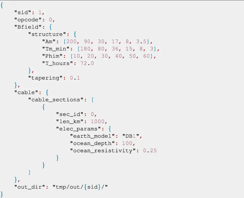
Listing 1

Listing 1. Example Input Control JSON. A few example input control JSONs can be found here.The parameters shown in Listing 1 are described in Table 5. In the listing the submarine cable related details are given under ‘cable’ parameter, which describes the cables into multiple cable section under ‘cable_sections’ parameter. Each entry in cable section holds the details about the cable segment, such as length of cable or the location information of cable section ends, and electrical properties etc. The electrical properties hold the information about the thickness and resistivity details of the Ocean-Earth layers. In addition, each cable section also holds information about the INTERMAGNET station name, which is used to extract B-field data and compute induced E-field and cable voltage using the DSTL model. This example Control JSON creates synthetic magnetic field data (see Section 2.4.2 for details) and transfer functions based on the electrical properties of the Ocean-Earth structure, along the cable section, provided by the cable. cable_sections[0]. elect_params JSON field. The cable_sections[i] fields also provide physical information on the cable, such as effective length (len_km) or Northward/Eastward geodetic lengths of the cable sections or geodetic location information of the cable route. In-built intelligence of the software can parse any of this information to estimate effective length of the cable. For a detailed description of all the available JSON fields, please refer to the Supplementary Document.

TABLE 5

TABLE 5. Description of the parameters presented in Control JSON Listing 1.

3.2 Compatibility & operating system

The software is written in Python-3.10 language, thus it is compatible with any Python code or interpretor or distribution. However, there are ways to invoke/embed the model functionalities from other languages. Specifically, codes written in Python-3.10 can be embedded into C/C++. Due to its complicated embedding structure, we encourage users to invoke the software from the Python-3.*.* environment. In addition, the code consumes less memory, computational unit, and can run in Unix, Windows, and MAC operating systems.

3.3 Helper python-packages used in the code

The majority of analysis and visualization was completed with the help of free, open-source software tools such as numpy [23], scipy [24], matplotlib [25], IPython [26], pandas (e.g. [27, 28]).

3.3.1 Calculation of seafloor transfer function (T_x) using BEZpy

The calculation of induced geoelectric fields during geomagnetic storms is a long studied problem. The transfer function described in Eq. 2 requires computation of effective reflection coefficients for each layer of the Earth to calculate the seafloor impedance. The calculation of effective reflection coefficients for layered Earth structure can be done using recursive function call. BEZpy [29,30] is primarily implemented for analysis of magnetic (B), electric (E), and impedance (Z) data within a geophysical framework. This library contains routines for calculating the geoelectric field from the geomagnetic field in multiple ways. BEZpy implements the recursive function procedure to compute effective reflection coefficients and impedance at the seafloor. The BEZpy Python code is released under a BSD-3 license, hence, we used this module as a plugin into our Python code, to simplify the effective seafloor impedance (Z) calculation.

4 Results

This section presents the outputs, namely, transfer functions T_x, induced emf ${\mathcal{E}}_C$, total voltage U_C for the following cases: 1) uniform and Atlantic Ocean-Earth conductivity model, 2) electrically-long and electrically-short Ocean-Earth sections, 3) effects of variations in seawater depth, d, on the transfer function, T_x and 4) effects of variations in seawater depth, d, on transmission line parameters. We used the synthetic magnetic field data presented in Section 2.4.2 for all the above-listed case study simulations. In addition, we link the GitHub code base for sample code and example Input Control JSON.

4.1 Uniform, and Atlantic Ocean-Earth conductivity model

To validate the model performance, we compare the estimations of the induced seafloor electric fields (E_f) from the model with corresponding analytical solutions for two different Ocean-Earth Conductivity models. For the analysis, we have used the following conductivity models: 1) uniform: consisting of equal σ for all the layers and 2) the Atlantic conductivity model presented in Table 2. Figure 5 presents the comparisons to validate the model forecast using synthetic magnetic field data (refer Section 2.4.2). From top to bottom of Figure 5, the rows present a) transfer function, b) induced electric field estimates from the model and their analytical solutions, and c) correlation analysis between the electric field estimates. For all the cases, the model is able to reproduce the analytical solution (refer to ρ provided in panels (c-1 ∼2)). Note that, electric fields estimated using the model (E_n(t)) presented in panels (b-1 ∼2) are tapered around their edges, which is due to the tapering of the input magnetic field. The tapering reduces the spurious frequency components in the data and produces a smooth output. Thus, while conducting the correlation analysis we removed the edges from both E(t) estimates. The correlation coefficient (ρ) is shown in the top left corners in the bottom row (panels (c-1 ∼2)). From correlation analysis we find that there is a 1 in 10⁶ part difference between the numerical estimates and analytical solution, indicating a high confidence in the model calculations. This comparative analysis shows that the model is sensitive to the Ocean-Earth layered conductivity structure.

FIGURE 5

FIGURE 5. Model validation using following layered Ocean-Earth conductivity models: 1) Uniform and 2) Atlantic model described in Table 2. From top to bottom rows present: (A) Amplitude and phase spectrum of the transfer function, T_x. (B) Time series of analytically (red) and numerically (black) estimated induced electric field. (C) Correlation analysis between analytically (E_a(t)) and numerically (E_n(t)) calculated induced electric field. The correlation coefficient (ρ) between E_a(t) and E_n(t) is provided in the top left corner of the panel. Example Python notebook for this experiment is uploaded in Zenodo [21].

4.2 Electrically-long and electrically-short Ocean-Earth sections

In this case study, we validate Ocean-Earth potential estimates from the model against the standard theoretical solution presented in Section 2.4.1. Figure 6 presents the outputs for 1) electrically-short and 2) electrically-long Ocean-Earth sections. For this analysis we used the Ocean-Earth layered conductivity model described in Table 2, which has the amplitude and phase spectrum of the transfer function. We use an input electric field of E_f = 1 mV/km. The Earth potential, estimated from the model (in black “+“), is overlaid on top of the analytical solutions (in red). The correlation analysis indicates a 1 in 10⁹ part difference between the numerical estimates and analytical solution for both the cases under consideration indicating a high confidence in the modeling process.

FIGURE 6

FIGURE 6. Distribution of voltage, estimated using theoretical approximation (red) and computational model (black “+”), along the (A) electrically-short and (B) electrically-long Ocean-Earth sections. The correlation coefficient between theoretical and numerical estimates are provided in each panel. L and $\frac{1}{\gamma }$ are the physical length and adjustment distance of the cable, respectively. Example Python notebook for this experiment is uploaded in Zenodo [21].

4.3 Effects of variations in seawater depth, d, on the transfer function, T_x

Among the various model parameters, seawater depth is the one that has the most influence on the seafloor electric field. Here, we conduct a sensitivity analysis, presented in Figure 7, that shows how change in sea-water depth impacts the amplitude (top panel) and phase (bottom panel) of the transfer function. This shows that changing the seawater depth can change the transfer function amplitudes by orders of magnitude. In addition, we observe the following features in the amplitude spectrum: 1) tapering for higher frequency increases with seawater depth, indicating a water shielding effect, 2) at lower frequencies all amplitude spectra converge and taper off to lower values, indicating an attenuation for the waves with very long periods, irrespective of the seawater depth. From the phase spectrum we observe a stable progression of phase change from 70° to 0° for the frequency range under consideration.

FIGURE 7

FIGURE 7. (A) Amplitude and (B) phase of the transfer functions T_x for different seawater depths (D). Example Python notebook for this experiment is uploaded Zenodo [21].

4.4 Effects of variations in seawater depth, d, on transmission line parameters $Z_0\text{\hspace{0.17em}and\hspace{0.17em}}\frac{1}{\gamma }$

Variations in seawater depth also impact the transmission line model parameters (refer to Supplementary Document: Module 03). In Figure 8 we present the variations of characteristic impedance Z₀ (in red ‘+’) and adjustment distance $\frac{1}{\gamma }$ (in blue squares) of the transmission line model for a fixed layered Earth presented in Table 2 (except the top row). Note that, as expected (refer to Supplementary Document: Module 03) the characteristic impedance (Z₀) and propagation constant (γ) of the transmission line model decreases with increasing seawater depth (d). Supplementary Equations S1–S6 indicate that an increase in seawater depth increases the horizontal conductance C and, subsequently, reduces the series impedance Z, which finally reduce the characteristic impedance (Z₀) and propagation constant (γ) of the transmission line. Supplementary Equations S1–S6 also indicate that the relation between series conductance C and Z₀, γ is hyperbolic in nature, hence, we observe the same trend in the output presented by Figure 8.

FIGURE 8

FIGURE 8. (Red) Characteristic impedance (Z₀) and (Blue) adjustment distance $(\frac{1}{\gamma })$ of the transmission line model for different seawater depths (D). Example Python notebook for this experiment is uploaded in Zenodo [21].

5 Discussion

Here, we presented a computational model that is capable of estimating geomagnetically induced electric fields at the seafloor and associated voltages in submarine cables and that can be used to examine the magnetic induction effects due to various types of geomagnetic field variations. We describe the Python software that does all the computation, all the inputs required to run the model, and show how the shielding effects of the seawater and the Ocean/Earth conductivity structure affects the results. To test the modeling software we make calculations using a synthetic magnetic perturbation as input, and validate the model output by comparison with analytic solutions. In future work we plan to use the model to make calculations of the induced voltages in the TAT-8 trans-Atlantic cable and compare these to measurements made during the March 1989 geomagnetic storm.

The magnetic induction model consists of two primary parts, first, a transfer function that calculates geomagnetically induced electric field at the seafloor; second, a calculation of seafloor Earth potential due to induced electric field using a transmission line model of the Ocean/Earth conductivity structure. There are a number of different types of magnetic field variations: all will induce an electric field in submarine cables, but not all of them have the characteristics to produce electric fields that may be important for submarine cable operation. From the transfer functions we can directly understand that the layered Ocean-Earth acts like a band-pass filter, that allows magnetic disturbance with specific periods to induce electric field under the sea. This helps us to infer what types of magnetic phenomena may affect submarine cable infrastructures. Thus this model can be used to study the effects of many types of geomagnetic disturbances on submarine cables, including storm sudden commencements (SSC) [31], magnetic storm main phase [32], and magnetic substorms [33].

5.1 Assumptions and limitations of the model

All the model assumptions and limitations contribute to the uncertainty of the model outputs. The one-dimensional (1-D) model assumes that the conductivity variations of the Ocean-Earth layers are only a function of depth and there are no lateral spatial conductivity variations within a given section. The seafloor geoelectric field calculations are made in a “piecewise” fashion [34] for each section, ignoring the sections on either side. The change between section are then handled by the transmission-line modeling. In addition, we assume that conductivity of the layers (including seawater and Earth) do not changes between each cable sections, which also contributes to the model uncertainty. One can reduce the section lengths to more closely follow the variations in ocean depth, but this violates the assumptions of 1-D induction theory, which assumes variations of conductivity and layer thickness in the east-west and north-south direction have negligible impact on the overall calculation. Moreover, calculating the Ocean-Earth layered conductivity model using LITHO1.0 interpolates thicknesses of layers at the middle point of a cable segment, which produces an interpolation error that also contributes to the model uncertainty. Note that, the cable route is split into sections to capture the large-scale changes in the cable depth, so that there are only small changes in depth within each section.

Several factors act together to influence the size of the voltage variations encountered by submarine cables. The magnetic field at the sea surface has a spectrum that falls off with frequency, whereas the transfer function between the seafloor electric field and surface magnetic field increases with frequency for shallow sea depths such as on the continental shelf, while the response to deep ocean seafloor is flatter. In the deep ocean, higher frequencies do not contribute as much to the electric fields on the seafloor. Another important factor is the spatial extent of the magnetic disturbances. Trans-oceanic submarine cables span large distances that cover many time zones, so the magnetic disturbances at opposite ends of a cable are not necessarily the same. Besides, it is also hard to find magnetometer stations (observations) near the submarine cable route across the ocean. Thus, the model has to interpolate sparsely available magnetometer data along the cable route, which is another source of uncertainty in the calculations. These factors all needed to be examined on a case-by-case basis for specific cables. This is planned to be a topic of future work using the modeling tools described in this paper.

6 Conclusion

In this study, we present a computational model to estimate the geomagnetically induced electric field and voltage in submarine cables. This includes calculation of the transfer function relating the seafloor electric field to the surface magnetic field variations. Cross-ocean modeling describes a way to estimate induced voltage along the submarine cable due to the seafloor geoelectric field. A synthetic geomagnetic field has been defined, comprising six frequency components, to validate the model performance against theoretical outputs. We validated the model calculation processes by comparison of model results with analytic solutions for two different Ocean-Earth conductivity models and electrically-long and electrically-short Ocean-Earth sections. The induced geoelectric field at the seafloor and induced voltage within the cable are directly related to the seawater depth. The sensitivity study indicates that the seawater layer acts as a shield in the induction process: the greater the ocean depth, the smaller the seafloor geoelectric field. In addition, we found that the model is sensitive to the Ocean-Earth layered conductivity structure. Thus, the geomagnetic effect on submarine cables depends on the intensity of the geomagnetic disturbance at that location on the globe as well as the seawater depth and Ocean-Earth layered conductivity structure along the cable route. The model can be used to study the effects of different types of geomagnetic phenomena including SSC, storm main phase, substorms etc. The present modeling incorporates various simplifying assumptions, such as the use of 1-D Earth conductivity models. Possible improvements to the modeling could include use of 3-D finite element models to more accurately represent the variations of ocean depth and conductivity structure along the cable route.

Data availability statement

The datasets used in this study are synthetically produced inside the code and can be found in the GitHub code repository identified by the following https://github.com/shibaji7/submarine_cable_modeling.git. The latest version of the code is published in Zenodo [21]. The example code and IPython notebooks are also available in Zenodo and GitHub repositories. The crust and lithospheric model of the Earth LITHO1.0 model [9] is available on IRIS DMC Data Products website [35].

Author contributions

SC contributed to code writing, model validation, analysis, and drafting the manuscript. DB, XS, and MH contributed to conception and design of the study. BM contributed to conductivity modeling. XW, GL, and JB provided feedback on manuscript organization. All authors contributed to manuscript revision, read, and approved the submitted version.

Funding

SC, XS, MH, and JB were supported by NASA 80NSSC19K0907 and 80NSSC21K1677. DB was supported by Natural Resources Canada contribution number 20220247. SC and XS also thank the National Science Foundation for support under grants AGS-1935110. BM was supported by a Mendenhall Postdoctoral Fellowship through the U.S. Geological Survey.

Acknowledgments

Authors acknowledge Josh Rigler, Krissy Lewis, Ryan Gold, and Janet Carter for facilitating USGS internal review. Any use of trade, firm, or product names are for descriptive purposes only and does not imply endorsement by the U.S. Government.

Conflict of interest

The authors declare that the research was conducted in the absence of any commercial or financial relationships that could be construed as a potential conflict of interest.

Publisher’s note

All claims expressed in this article are solely those of the authors and do not necessarily represent those of their affiliated organizations, or those of the publisher, the editors and the reviewers. Any product that may be evaluated in this article, or claim that may be made by its manufacturer, is not guaranteed or endorsed by the publisher.

Supplementary material

The Supplementary Material for this article can be found online at: https://www.frontiersin.org/articles/10.3389/fphy.2022.1022475/full#supplementary-material

References

1. Carter L, Burnett D, Drew S, Hagadorn L, Marle G, Bartlett-Mcneil D, et al. Submarine cables and the oceans – connecting the world. Kenya: UNEP-WCMC Biodiversity (2009).

Google Scholar

2. Boteler D, Pirjola R, Nevanlinna H. The effects of geomagnetic disturbances on electrical systems at the Earth’s surface. Adv Space Res (1998) 22:17–27. Terrestrial Relations: Predicting the Effects on the Near-Earth Environment. doi:10.1016/S0273-1177(97)01096-X

CrossRef Full Text | Google Scholar

3. Prescott G. Observations made at boston, mass., and vicinity, in article on the great auroral exhibition of august 28th to september 4th, 1859. Amer J Sci Arts (1860) 92–7.

Google Scholar

4. Prescott G. History, Theory and Practice of the electric telegraph (ticknor and fields). London: the University of Michigan (1866).

Google Scholar

5. Boteler D. The super storms of august/september 1859 and their effects on the telegraph system. Adv Space Res (2006) 38:159–72. The Great Historical Geomagnetic Storm of 1859: A Modern Look. doi:10.1016/j.asr.2006.01.013

CrossRef Full Text | Google Scholar

6. Anderson CW. Magnetic storms and cable communications, solar system plasma Physics (kennel, C) (1978).

Google Scholar

7. Lanzerotti LJ. Geomagnetic induction effects in ground-based systems. Space Sci Rev (1983) 34:347–56. doi:10.1007/BF00175289

CrossRef Full Text | Google Scholar

8. Medford LV, Lanzerotti LJ, Kraus JS, Maclennan CG. Transatlantic Earth potential variations during the march 1989 magnetic storms. Geophys Res Lett (1989) 16:1145–8. doi:10.1029/GL016i010p01145

CrossRef Full Text | Google Scholar

9. Pasyanos ME, Masters TG, Laske G, Ma Z. Litho1.0: An updated crust and lithospheric model of the Earth. J Geophys Res Solid Earth (2014) 119:2153–73. doi:10.1002/2013JB010626

CrossRef Full Text | Google Scholar

10. Cox C. Electromagnetic induction in the oceans and inferences on the constitution of the Earth. Geophys Surv (1980) 4:137–56. doi:10.1007/BF01452963

CrossRef Full Text | Google Scholar

11. Medford LV, Meloni A, Lanzerotti LJ, Gregori GP. Geomagnetic induction on a transatlantic communications cable. Nature (1981) 290:392–3. doi:10.1038/290392a0

CrossRef Full Text | Google Scholar

12. Dawson TW, Weaver JT, Raval U. B-polarization induction in two generalized thin sheets at the surface of a conducting half-space. Geophys J Int (1982) 69:209–34. doi:10.1111/j.1365-246X.1982.tb04945.x

CrossRef Full Text | Google Scholar

13. Boteler DH, Pirjola RJ. Magnetic and electric fields produced in the sea during geomagnetic disturbances. Pure Appl Geophys (2003) 160:1695–716. doi:10.1007/s00024-003-2372-6

CrossRef Full Text | Google Scholar

14. Peltier A, Chulliat A. On the feasibility of promptly producing quasi-definitive magnetic observatory data. Earth Planets Space (2010) 62:e5–8. doi:10.5047/eps.2010.02.002

CrossRef Full Text | Google Scholar

15. Wang S, Constable S, Rychert CA, Harmon N. A lithosphere-asthenosphere boundary and partial melt estimated using marine magnetotelluric data at the central middle atlantic ridge. Geochem Geophys Geosyst (2020) 21:e2020GC009177. doi:10.1029/2020gc009177

CrossRef Full Text | Google Scholar

16. Rychert CA, Tharimena S, Harmon N, Wang S, Constable S, Kendall JM, et al. A dynamic lithosphere–asthenosphere boundary near the equatorial mid-atlantic ridge. Earth Planet Sci Lett (2021) 566:116949. doi:10.1016/j.epsl.2021.116949

CrossRef Full Text | Google Scholar

17. Attias E, Evans RL, Naif S, Elsenbeck J, Key K. Conductivity structure of the lithosphere-asthenosphere boundary beneath the eastern north American margin. Geochem Geophys Geosyst (2017) 18:676–96. doi:10.1002/2016GC006667

CrossRef Full Text | Google Scholar

18. Grayver AV. Global 3-d electrical conductivity model of the world ocean and marine sediments. Geochem Geophys Geosyst (2021) 22:e2021GC009950. doi:10.1029/2021gc009950

CrossRef Full Text | Google Scholar

19. Boteler DH, Pirjola RJ. Numerical calculation of geoelectric fields that affect critical infrastructure. Int J Geosciences (2019) 10:930–49. doi:10.4236/ijg.2019.1010053

CrossRef Full Text | Google Scholar

20. Horton R, Boteler D, Overbye TJ, Pirjola R, Dugan RC. A test case for the calculation of geomagnetically induced currents. IEEE Trans Power Deliv (2012) 27:2368–73. doi:10.1109/TPWRD.2012.2206407

CrossRef Full Text | Google Scholar

21.[Dataset] Chakraborty S (2022). shibaji7/submarine_cable_modeling: Geomagnetic Induction in Submarine Cables. doi:10.5281/zenodo.7055321

CrossRef Full Text | Google Scholar

22. Boteler DH, Pirjola RJ, Marti L. Analytic calculation of geoelectric fields due to geomagnetic disturbances: A test case. IEEE Access (2019) 7:147029–37. doi:10.1109/ACCESS.2019.2945530

CrossRef Full Text | Google Scholar

23. Harris CR, Millman KJ, van der Walt SJ, Gommers R, Virtanen P, Cournapeau D, et al. Array programming with NumPy. Nature (2020) 585:357–62. doi:10.1038/s41586-020-2649-2

PubMed Abstract | CrossRef Full Text | Google Scholar

24. Virtanen P, Gommers R, Oliphant TE, Haberland M, Reddy T, Cournapeau D, et al. SciPy 1.0: Fundamental algorithms for scientific computing in Python. Nat Methods (2020) 17:261–72. doi:10.1038/s41592-019-0686-2

PubMed Abstract | CrossRef Full Text | Google Scholar

25. Hunter JD. Matplotlib: A 2D graphics environment. Comput Sci Eng (2007) 9:90–5. doi:10.1109/MCSE.2007.55

CrossRef Full Text | Google Scholar

26. Perez F, Granger BE. Ipython: A system for interactive scientific computing. Comput Sci Eng (2007) 9:21–9. doi:10.1109/MCSE.2007.53

CrossRef Full Text | Google Scholar

27. McKinney W. Data structures for statistical computing in Python. In: S van der Walt, and J Millman, editors. Proceedings of the 9th Python in science conference (2010). p. 56–61. doi:10.25080/Majora-92bf1922-012

CrossRef Full Text | Google Scholar

28. Millman KJ, Aivazis M. Python for scientists and engineers. Comput Sci Eng (2011) 13:9–12. doi:10.1109/MCSE.2011.36

CrossRef Full Text | Google Scholar

29.[Dataset] Lucas G. greglucas/bezpy. Hawaii: First release of bezpy (2020). doi:10.5281/zenodo.3765861

CrossRef Full Text | Google Scholar

30. Love JJ, Lucas GM, Kelbert A, Bedrosian PA. Geoelectric hazard maps for the mid-atlantic United States: 100 year extreme values and the 1989 magnetic storm. Geophys Res Lett (2018) 45:5–14. doi:10.1002/2017GL076042

CrossRef Full Text | Google Scholar

31. Zhang JJ, Yu YQ, Wang C, Du D, Wei D, Liu LG. Measurements and simulations of the geomagnetically induced currents in low-latitude power networks during geomagnetic storms. Space Weather (2020) 18:e2020SW002549. doi:10.1029/2020sw002549

CrossRef Full Text | Google Scholar

32. Rajput VN, Boteler DH, Rana N, Saiyed M, Anjana S, Shah M. Insight into impact of geomagnetically induced currents on power systems: Overview, challenges and mitigation. Electric Power Syst Res (2021) 192:106927. doi:10.1016/j.epsr.2020.106927

CrossRef Full Text | Google Scholar

33. Viljanen A, Tanskanen EI, Pulkkinen A. Relation between substorm characteristics and rapid temporal variations of the ground magnetic field. Ann Geophys (2006) 24:725–33. doi:10.5194/angeo-24-725-2006

CrossRef Full Text | Google Scholar

34. Marti L, Yiu C, Rezaei-Zare A, Boteler D. Simulation of geomagnetically induced currents with piecewise layered-Earth models. IEEE Trans Power Deliv (2014) 29:1886–93. doi:10.1109/TPWRD.2014.2317851

CrossRef Full Text | Google Scholar

35. Trabant C, Hutko AR, Bahavar M, Karstens R, Ahern T, Aster R. Data products at the IRIS DMC: Stepping stones for research and other applications. Seismological Res Lett (2012) 83:846–54. doi:10.1785/0220120032

CrossRef Full Text | Google Scholar

36. Wang X, Boteler D, Pirjola R. Distributed-source transmission line theory for modeling the coast effect on geoelectric fields. IEEE Trans Power Deliv (2022).

Google Scholar