A Fractal Theory of Urban Growth

This paper presents an analytical framework for the physical environment of cities using fractal theory. The strength of the approach lies in its simplicity and precision. The equations presented in this article comprise: the number of occupied sites in an area; the population and the length of roads of a city; its fractal dimension; its number of average and maximum levels (floors per building); the average density of population and roads; what are the limits to growth as well as an analysis on some of the city’s scaling laws. These equations describe to a high level of precision the real values measured in the system of the United Kingdom, for every city above 5,000 people, which amounts to a sample size of 1,031 cities. This work will allow further research into the nature of cities, since it enables the creation of synthetic cities, and further analytical derivations that can arise from these building blocks. The paper shows as well how the same set of equations can be used to characterise the internal distribution of cities from the perspective of its growth as a possible example of an application of the framework.

Introduction

The field of urban studies is a continuous pursuit for regularities that expand our capacity to describe and understand cities. From its origins, the field has been intimately related to ideas and methodologies in the field of statistical physics, and an overarching summary of the path and main ideas of the application of statistical physics to urban environments is presented in [1].

We cannot claim that we understand how cities evolve as long as we do not have an exact set of equations that relate every variable to each other allowing us to understand the effects of population growth. This is paramount for a large number of fields, including research, urbanism and political/economical science. The aim of this work is to create an analytical framework for the analysis of the most important variables in a city from a geometrical standpoint.

This paper presents a theory of the physical aspect of the city using a fractal framework. Cities are defined by their occupation of space, and I show over the next sections that cities increase their fractal dimension as they grow in population, which is a fundamental property, and which was already noted in [2]. In fact, the study of cities as fractals has a long tradition in the scientific literature [2–8]. This view is fundamental to understand cities, since it commands the occupation of space for a given city, and therefore it is the only valid way to extract its geometric framework.

The work presented in this paper studies the population, the road network, the occupation of space, the fractal dimension of the city, the average heights, the maximum heights and the interactions or GDP of a city. I show how all these variables are related between each other and how they were derived. This work is not the first to attempt to produce a set of equations that describe the main variables of the city. Some previous work include [9, 10] which show how congestion influence the growth of cities, the aforementioned [2] that presents a theory of growth of cities based on scaling theory or several theories on the growth of cities [11–13].

This work delves as well into how this fractal framework affects and influence the scaling of a number of variables. Scaling theory [14–17] in urban science [18–23] study how allometric relations appear between variables such as the length of roads, the number of gas stations, the cost of maintaining a city’s infrastructure, its GDP and many other quantities to the size of the city in terms of population. In previous work [24], it was shown that those scaling exponents could be derived from a simplified and approximated version of the equations that governed those same variables. The current work presents an improvement on the calculation of the scaling exponents going beyond what was presented in [24], since we now account with better and more precise equations to describe length of roads, population and GDP.

The work also shows an application of the set of formulas to develop an approximation of the internal distribution of a city, derived from its growth. In order to do so, it assumes that the same formulas that describe a city in its current state have to remain meaningful to describe a city at any specific instant of its history, meaning that this growth is ergodic.

Framework

Cities begin to form with the construction of a single house, slowly other houses join, percolating space, and soon the city’s fractal dimension starts increasing. New occupied sites are incorporated with a certain probability of occupation over the territory that surrounds the city while the existing urban fabric gets densified. This probability of occupation tends to a constant value because of a self-optimization pattern. Going any lower would break the city apart into different clusters and expand the city over a long area, increasing travel times and decreasing economies of scale. Going higher would increase traffic and other problems derived from density, leading to an optimal solution in which the probability of occupation is as low as possible while still keeping the city as one single cluster. This probability is very close to the critical probability of a percolation over a squared lattice in two dimensions because the topology of cities is in average similar to that lattice.

In its first stages the city densifies its road network, subdividing the occupied sites which increases the density of occupation. At some point in its growth, the density of people that can live in a planar city saturates and in order to keep growing, the city needs to extend into the third dimension increasing its height, eventually pushing the fractal dimension of the population above 2. From its initial state, the density of population keeps on ever increasing as the city first densifies and later grows further into the third dimension.

The current section constructs the main framework of this work, presenting the derivation of its equations for several geometrical variables in a city. In order to simplify the equations and reasoning, I will use along this section an idealised system, in which I will avoid talking about multipliers or characteristic scales that need to be fitted in order to obtain realistic values, I will show how to calculate those multipliers in the last section of the paper, where I will adapt the equations to work with a real system and give the value for the constants in the specific case of the United Kingdom which will serve as an example throughout the paper.

As a city grows, the pre-existing city does not disappear, meaning that it must maintain a minimum of the current probability of occupation of sites where buildings are constructed. Considering a squared city with a linear dimension L, with a planar fractal dimension d and a certain number of occupied sites n = L^d (shown in Figure 1B) coming from a probability of occupation ρ over an area a = L². Then we have ρa = n which in turn means that L^d−2 = ρ so:

$d=2+\frac{\ln \left(\rho \right)}{\ln \left(L\right)}(1)$

FIGURE 1

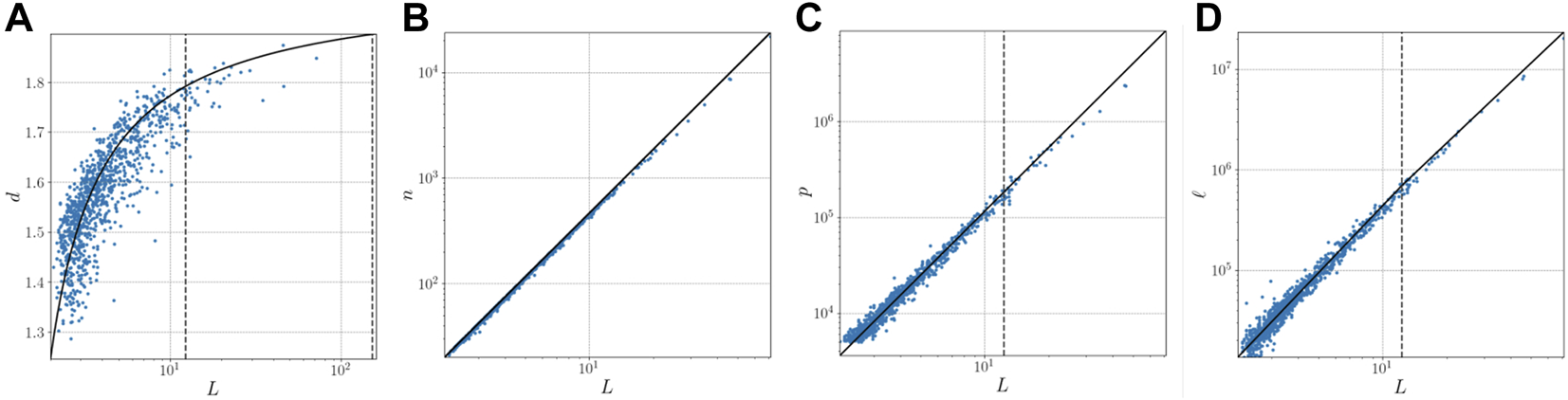
FIGURE 1. Comparison between real data and their corresponding equations. (A) fractal dimension as a function of linear dimension of the city. (B) number of occupied sites as a function of the linear dimension of the city, measured using GHS data [26]. (C) population as a function of the linear dimension of the city from GHS data. (D) total length of roads as a funcion of the linear dimension of the city taken from OSM data [28]. In blue real data, in black the equations derived with this approach. The vertical dotted line corresponds with the critical threshold.

This equation means that the fractal dimension of a city needs to increase as its linear dimension grows in order to avoid having its preexisting city disappear, this was already noted in [2]. Otherwise, if it were to remain constant (or decrease) we see that the only solution would be to decrease its probability of occupation, meaning that in order to occupy sites in its outskirts the city would need to vacate sites in its preexisting city. This explains the behaviour observed in real systems (Figure 1A) which shows a normal distribution of the error between the predicted and real value with mean −0.0142 and standard deviation of 0.0677.

Cities grow vertically above its two-dimensional footprint. In fact, population becomes a fractal volume, that starts below dimension 2 but as cities become larger it surpasses it. Furthermore, the population has always a larger fractal dimension than the footprint of a city. As it was shown on [24] the fractal dimension of the population (d_p) can be obtained by adding a fractal vertical component η to the planar fractal dimension of sites d, that is d_p = d + η and therefore the population (shown in Figure 1C) can be expressed as

$p=L^{d+\eta }(2)$

Throughout its growth, a city starts densifying its street network increasing the quantity of people that can live within it, and at some threshold x_c the density of population per site in a planar city saturates and cannot longer continue growing through this process. In order to keep on growing above that critical threshold x_c it needs to start increasing its height. Therefore, the growth of people per site $\frac{p}{n}=L^{\eta }$ is absorbed either by the increase in average length of roads ⟨ℓ⟩ in a site of the space of the city or by the average number of vertical levels (floors) of the city ⟨h⟩. This means that

$\frac{p}{n\langle \ell \rangle \langle h\rangle }=k(3)$

is a constant.

Numerically, at x_c, the density of roads reaches its maximum value of 1 (understood as the probability of finding a road segment in a site) ⟨ℓ⟩_c = 1 and the average number of levels of the city is also 1, ⟨h⟩_c = 1, since it was 1 from the beginning of the growth of the city and it only starts increasing right after x_c. So we have that:

$\langle {\ell \rangle }_c\langle {h\rangle }_c=1=\frac{p_c}{k{n}_c}=\frac{1}{k}{L}_c^{\eta }(4)$

We also have that since ρa = n,

$\frac{p}{a\langle \ell \rangle \langle h\rangle }=\rho k(5)$

This last equation means that at x_c the population is proportional to the area since ⟨ℓ⟩_c = 1 and ⟨h⟩_c = 1 and k and ρ are constants. Therefore, the fractal dimension of the population at x_c is the same as the fractal dimension of the area $(d_{p_c}=d_c+\eta =2)$. In other terms, at the point in which the population starts growing into the third dimension is the threshold in which its fractal dimension grows above 2, as expected. We can see that since at x_c, d_c = 2 − η and using Eq. 1 we have that η is

$\eta =-\frac{\log \left(\rho \right)}{\log \left(L_c\right)}(6)$

and since p_c = L² = a_c and a/n = ρ⁻¹ then $L_c^{\eta }=p_c/n_c={\rho }^{-1}$, therefore, we can see that our constant in Eq. 4 is k = ρ⁻¹ which means that,

$\frac{p}{n\langle \ell \rangle \langle h\rangle }={\rho }^{-1}(7)$

for any city size. This is a constant for any city, the limit of population density in each vertical floor belonging to a site per meter of road (how dense is the network, how subdivided is the system), the system cannot hold more people than this value per site, per level. Furthermore, Eq. 5 becomes

$\frac{p}{a\langle \ell \rangle \langle h\rangle }=1(8)$

which means that at the critical threshold x_c, when saturation is reached and both the density of roads and the number of levels is 1, the population equals the area. Moreover, and as an indirect consequence of Eq. 6 we also have that the threshold x_c is reached when the linear dimension of the city is L_c = ρ^−1/η.

A city cannot grow without limit, the equations portrayed in this work show that its density would go to impossible amounts, the heights of its buildings would reach levels that are physically unattainable and a large number of other issues such as congestion and competition for space would arise. As we see in Eq. 7, ρ⁻¹ is the density limit for the night time population, how many people can live in each site per level, and this is a hard limit, no city outgrows this. As cities grow further than this threshold (x_c), the day-time population will spread over its area, people will walk down the parks, the plazas, the avenues and will of course be present in buildings. Since the area of the city cannot contain several levels, it means that at some point in its growth, the population spread over its area will also reach this same limit $\frac{p}{a}={\rho }^{-1}$ and the city will be completely collapsed. This is expectedly a hard limit for growth, and cities will not surpass it. In fact, using our equations and the multiplying factors measured for the United Kingdom, this only happens when the population of a city reaches 36.1 million people, and the largest city on Earth has a very similar level of population, of course, this is a numerical result that is highly dependent on the approximated value of η and ρ obtained through a genetic algorithm as explained in the next section, and very slight modifications to those values change greatly this specific value. We call this maximum threshold x_m.

If at x_m we have that ρp_m = a_m and for all cities ρa = n, then $\frac{p_m}{n_m}=L_m^{\eta }={\rho }^{-2}$ which means that L_m = ρ^−2/η and using Eq. 1, d_m = 2 − η/2.

Regarding ⟨ℓ⟩ and ⟨h⟩ given that we know that both are complementary, since at x_c both are 1, and one cannot exist in the numeric range of the other (one has to be less than 1 and the other more than 1) then we have that $⟨h⟩⟨\ell ⟩=\frac{p}{a}=\rho \frac{p}{n}=\rho L^{\eta }={\rho }^{1+\frac{\eta }{d-2}}$ and given that ⟨ℓ⟩ is a probability and cannot go above the value 1:

$⟨\ell ⟩=\min \left({\rho }^{1+\frac{\eta }{d-2}},1\right)=\min \left(L^{d+\eta -2},1\right)(9)$

which is shown in Figure 2D, and since $⟨h⟩=\rho \frac{p}{n⟨\ell ⟩}$ then:

$⟨h⟩=\max \left(1,\rho L^{\eta }\right)=\max \left(1,{\rho }^{1+\frac{\eta }{d-2}}\right)=\max \left(1,L^{d+\eta -2}\right)(10)$

portrayed in Figure 2B.

FIGURE 2

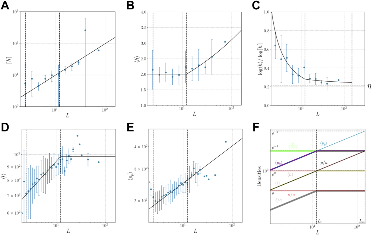
FIGURE 2. Comparison between number of levels and densities in the system with their respective equations. (A) maximum number of levels as a function of the linear dimension of the city. The number of levels is taken from data in Open Street Maps [28] (B) average number of levels as a function of the linear dimension of the city. (C) approximation of η using $\frac{\ln ⟨h⟩}{\ln \lceil h\rceil }$ which as we can see works only above x_c and will only reach exactly the same value as the true η (horizontal dotted line) at infinity. (D) average length of roads per site as a function of the linear dimension of a city. (E) planar density of the population per site as a function for the linear dimension of the city. (F) summary of how every density evolves as a function of the linear dimension of the city. In blue real data, in black the equations derived with this approach. The vertical dotted line corresponds with the critical threshold.

We can also obtain from Eq. 9 the total length of roads (shown in Figure 1D) which is:

$\ell =⟨\ell ⟩n=\min \left(1,{\rho }^{1+\frac{\eta }{d-2}}\right)L^d=\min \left(1,L^{d+\eta -2}\right)L^d(11)$

In order to calculate the maximum number of levels of the city (⌈h⌉) we use an approximation from [24] where we obtained that $d_p=d+\eta \sim d+\frac{\ln ⟨h⟩}{\ln \lceil h\rceil }$ using box counting analytically. Since this was only an approximation and meant to work above the critical threshold, we need to consider ⟨h⟩_x = ρL^η (without limiting its lower bound to 1). Doing so we have that $\eta \sim \frac{\ln ⟨h⟩}{\ln \lceil h\rceil }$ (Figure 2C) which means that $\lceil h\rceil \sim \exp (\frac{\ln (\rho L^n)}{\eta })\sim k_{h}L$. Because of the approximated nature of the equation we can not obtain directly the value of k_h and to calculate the true value of this multiplying constant we have to see that at the minimum possible linear dimension, when the city is composed of a single house, the average height and the maximum height should have the same value. This happens when d = 0, and since L = ρ^1/(d−2) then L_d=0 = ρ^−1/2, the average number of levels is ${⟨h⟩}_{d=0}=\rho L_{d=0}^{\eta }={\rho }^{1-\eta /2}$ and equating it to ⌈h⌉_d=0 = k_hL_d=0 = k_hρ^−1/2 we obtain that k_h = ρ^1.5−η/2 therefore:

$\lceil h\rceil ={\rho }^{1.5-\eta /2}L=L^{\frac{d\left(3-\eta \right)+\eta -1}{2}}(12)$

which is shown in Figure 2A.

We can also obtain equations that describe the average number of population in a site projected to the floor (collapsing all levels) ⟨p_p⟩ (Figure 2E), the average number of people per meter of road ⟨p_ℓ⟩ and the average number of people per site and per level ⟨p_h⟩

$⟨p_p⟩=\frac{p}{n}=L^{\eta }(13)$

$⟨p_l⟩=\frac{p}{l}=\max \left(L^{\eta },L^{d-2+2\eta }\right)(14)$

$\langle p_h\rangle =\frac{p}{n\langle h\rangle }=\min \left(L^{\eta },L^{d-2}\right)(15)$

Over the next sections I will show how to adapt this framework to real data and how to obtain the value of η and ρ to be able to get the final values of our exponents.

Scaling Theory

Originally a theory derived in the field of biology, scaling theory studies the allometric scaling of variables in a city as it they relate to its population growth. Some of those variables scale sub-linearly with the size of the city, meaning that the larger a city gets the slower that variable grows, this is the case for variables where economies of scale arise, such as the length of roads needed to cover the city, the number of gas stations, etc. Other variables grow linearly, because they correspond to some fixed value per person, such as the amount of water consumed. Finally, some other variables grow super-linearly, meaning that they grow faster than the population, usually these arise through feedback effects and include elements like traffic congestion, criminality, interactions or the GDP of a city. In [24] we showed that in fact, this relation to size was due to the fractal nature of cities, and calculated the expected exponents from the fractal scaling of the population and road network.

In that previous work [24] we reasoned that since the length of roads was proportional to L^d and the population was proportional to $L^{d_p}$, the scaling exponent should be equal to $\gamma =\frac{d}{d_p}=\frac{d}{d+\eta }$. We now have an improved formulation that describe both quantities and no longer need to make any approximations we can just solve the scaling equation ℓ = p^γ and calculate the exponent $\gamma =\frac{\ln \ell }{\ln p}$. This gives us that:

$\gamma =\min \left(\frac{d}{d+\eta },1+\frac{d-2}{d+\eta }\right)(16)$

this means that the previous reasoning still stands, but only for the largest cities (those above x_c) but the small cities are better represented by a different γ. The resulting length of roads fits the data to a very high degree of precision (normal distribution of the differences between the logged real and predicted values with μ = 0.01466 and σ = 0.1618) as shown in Figure 3A where Figure 3C shows the value of γ.

FIGURE 3

FIGURE 3. Relations between some of the variables and the scaling equations presented in this paper. (A) length of roads as a function of the population and the sublinear exponent (ℓ = p^γ). (B) GDP as a function of the population and the superlinear exponent $(\mathrm{G}\mathrm{D}\mathrm{P}=p^{{\gamma }_{\mathit{super}}})$. The GDP data was obtained from the Eurostat dataset [29] (C) values of both the sub-linear and super-linear exponents as calculated in this work. In blue real data, in black the equations derived using this approach. The vertical dotted line corresponds with the critical threshold.

In that same paper, we also reasoned that interactions occur when people go to the street and that therefore it should be proportional to the square of the quantity of people in the ground level, multiplied by the number of locations in which that were possible. In that work, the equations were approximated and we used ℓ ∼ n which gave us that i = (p/n) (p/n − 1)n, where i represents the total possible interactions, but since in this work we are distinguishing between the two values (ℓ and n), it is more precise to say that the people in the street interacts, and the number of possible locations is the length of the street network. therefore:

$i=\frac{p}{\ell }\left(\frac{p}{\ell }-1\right)\ell =p\left(\frac{p}{\ell }-1\right)=\max \left(L^{d+2\eta },L^{2+\eta }\right)-L^{d+\eta }(17)$

In order to obtain an approximation of the super-linear exponent of interaction $i\sim p^{{\gamma }_{\sup }}$, we need to drop the exact equation and approximate $i\sim {\left(\frac{p}{\ell }\right)}^2\ell =\frac{p^2}{\ell }=\frac{p^2}{p^{\gamma }}=p^{2-\gamma }$. Therefore the approximate value of the super-linear exponent is:

${\gamma }_{\sup }\sim 2-\gamma =\max \left(\frac{d+2\eta }{d+\eta },\frac{2+\eta }{d+\eta }\right)(18)$

Similarly to what was done in [24], we assume that the GDP of a city is a direct consequence of the interactions between individuals, and use that quantity to showcase the validity of the formulation as shown in Figure 3B while the super-linear exponent is shown in Figure 3C.

Formulation, Constants and Units for Real Data

The current framework represents an idealised system, it is unitless because everything is divided by an implicit characteristic scale that we will make explicit in this section and there are not any multiplying constants for the sake of simplicity. This section completes the framework, by including those factors and thus creating the final set of equations for the system.

From this point on forward we will use the subindex r to refer to real variables as measured from the data.

To determine the side of our real square (in meters) we use the area of the city.

$L_r=a_r^{\frac{1}{2}}(19)$

The characteristic scale for the length of the side of our squared area is called L₀ and it is measured in meters.

$L=\frac{L_r}{L_0}(20)$

where for the United Kingdom L₀ = 538.924 m. This value was calculated through measuring the fractal dimension for all cities and their areas. An approximation can be obtained through performing those measurements for the largest city (max (d_r), max (L_r)) and calculating our theoretical max(L) = exp (ln(ρ)/(max (d_r) − 2)), to find L₀ = max (L_r)/max(L). Of course, for this we need to determine ρ, this can be done either through directly measuring occupied space (buildings and roads) against open spaces in the city (parks, and plazas) or assuming our theoretical value for ρ = 0.5991 taken from the next section. As an example, London has an approximated 40% surface occupied by parks, which means that its ρ_r = 0.60. I use this value for L₀ as a starting guess and perform a least square estimate of L₀ using the measured fractal dimension and area for all cities (I assumed the theoretical ρ to be valid). Notice that we cannot use L_r and d to directly calculate ρ because. ${\rho }_r={(L_r/L_0)}^{d-2}\ne L_r^{d-2}$

For completeness, we will show how to obtain the area as a function of the side of the square.

$a_r=a_0{\left(\frac{L_r}{L_0}\right)}^2(21)$

where $a_0=L_0^2{\text{m}}^2$

$d=2+\frac{\ln \left(\rho \right)}{\ln \left(L_r/L_0\right)}(22)$

$p_r=p_0{\left(\frac{L_r}{L_0}\right)}^{d+\eta }(23)$

where for the United Kingdom p₀ = 1,207 people, which was measured by adjusting the theoretical population to the real data measured until their differences were minimised.

$n_r=n_0{\left(\frac{L_r}{L_0}\right)}^d(24)$

where for the United Kingdom n₀ = 7.85 sites, measured against the real data.

${\ell }_r={\ell }_0\min \left({\left(\frac{L_r}{L_0}\right)}^d,{\left(\frac{L_r}{L_0}\right)}^{2d+\eta -2}\right)(25)$

where for the United Kingdom ℓ₀ = 7,700 m, measured against the real data.

${⟨\ell ⟩}_r=\frac{{\ell }_0}{n_0}\min \left(1,{\left(\frac{L_r}{L_0}\right)}^{d+\eta -2}\right)(26)$

${⟨h⟩}_r=h_0\max \left(1,{\left(\frac{L_r}{L_0}\right)}^{d+\eta -2}\right)(27)$

where for the United Kingdom h₀ = 2 levels, measured against the real data.

$h_{m_r}=h_0{\left(\frac{L_r}{L_0}\right)}^{\frac{d\left(3-\eta \right)+\eta -1}{2}}(28)$

The constant that limits growth becomes:

$\frac{p_r}{{\ell }_r{⟨h⟩}_r}={\rho }^{-1}\frac{p_0}{{\ell }_0{h}_0}\frac{\text{people}}{\text{m\hspace{0.17em}level}}(29)$

and the densities:

$⟨p_{p_r}⟩=\frac{p_0}{n_0}{\left(\frac{L_r}{L_0}\right)}^{\eta }(30)$

$⟨p_{l_r}⟩=\frac{p_0}{l_0}\max \left({\left(\frac{L_r}{L_0}\right)}^{\eta },{\left(\frac{L_r}{L_0}\right)}^{d-2+2\eta }\right)(31)$

$⟨p_{h_r}⟩=\frac{p_0}{n_0{h}_0}\min \left({\left(\frac{L_r}{L_0}\right)}^{\eta },{\left(\frac{L_r}{L_0}\right)}^{d-2}\right)(32)$

Regarding the scaling equations, we have that the real length of the road network as a function of the real population becomes:

${\ell }_r={\ell }_0{\left(\frac{p_r}{p_0}\right)}^{\gamma }(33)$

Notice that, the typical equation of a scaling ${\ell }_r\propto p_r^{\gamma }$ is in fact ${\ell }_r=({\ell }_0/p_0^{\gamma })p_r^{\gamma }$, and since γ changes with the population size, the multiplying factor is not constant, as the equation ${\ell }_r\propto p_r^{\gamma }$ assumes. The fact that both the exponent and the multiplying factor vary with size explains a lot of the problematic that exists around measuring precisely the scaling exponent, although much of the variability becomes negligible if we only use cities above x_c.

For the GDP we have:

$g_r\sim g_0{\left(\frac{p_r}{p_0}\right)}^{2-\gamma }(34)$

where for the United Kingdom g₀ = 2.3 ⋅ 10⁷ euro, measured against the real data. This is an approximation, and from my perspective it is preferred to use the actual equation instead of an approximated scaling law, whenever possible, even though both equations look indistinguishable when presented against each other or the data. The equation for the interaction of population is:

$i_r=i_0\left(\max \left({\left(\frac{L_r}{L_0}\right)}^{d+2\eta },{\left(\frac{L_r}{L_0}\right)}^{2+\eta }\right)-{\left(\frac{L_r}{L_0}\right)}^{d+\eta }\right)(35)$

with a value i₀ unknown, since there is no data to measure it. This factor i₀ represents the probability that a potential interaction becomes a real one. Furthermore, if the assumption between proportionality of interactions and GDP stands:

$g_r=g_0\left(\max \left({\left(\frac{L_r}{L_0}\right)}^{d+2\eta },{\left(\frac{L_r}{L_0}\right)}^{2+\eta }\right)-{\left(\frac{L_r}{L_0}\right)}^{d+\eta }\right)(36)$

One interesting side effect of this, is that given that L₀, n₀, p₀, ℓ₀ and h₀ or even g₀ are pure constants for a system of cities (the variability is absorbed through the rest of the equation), they are much better descriptors of a system, and when calculated for other systems, they will allow us to make comparisons with less noise between different countries.

The Value of ρ and η

To render this analytical approach useful we need to be able to obtain the values of our two constants η and ρ. My approach was to use a genetic algorithm, whose inputs were the area (a_r, from where we obtain L_r), fractal dimension (d_r) and population (p_r) for each city and the parameters to be optimised are η_p and ρ_p. Using this, I apply a two steps approximation.

In the first step, in order to obtain the heuristic value for each individual, I calculate L₀ using the parameter ρ_p given by the algorithm, and then after calculating the real density ${\rho }_r={(L_r/L_0)}^{d_r-2}$ for each city, calculate an average density that mixes the parameter and the measured density, $\widehat{\rho }=({\rho }_p+{\rho }_r)/2$. I then calculate a theoretical fractal dimension $d=2+\ln (\widehat{\rho })/\ln (L_r/L_0)$ and obtain the theoretical population for each city using it $p={(L_r/L_0)}^{d+{\eta }_p}$, where η_p is the second parameter to be fitted by the algorithm. Then obtain the linear fit between the theoretical population p and the real one p_r = ap + b, discard b and return as the final heuristic the L1 norm between the logarithms of p_r and ap. In this phase we obtain the value of η and an approximation of the value of ρ.

In the second step, we fix η and only optimize ρ, allowing the search only in the neighborhood of the approximated value we obtained in the first step. The only difference between the two, is that we no longer use the real ρ_r and instead use directly the parameter ρ_p at every step (to calculate L₀ and d = 2 + ln (ρ_p)/ln (L_r/L₀)). From this second step we obtain our constant ρ.

The values obtained were:

$\eta =0.2092(37)$

$\rho =0.5991(38)$

were less significant digits were discarded. These values mean that d_m = 2 − η/2 = 1.8954 and d_c = 2 − η = 1.7908. The measurements of η and ρ were obtained from approximated processes and these measurements could be improved in the future.

This is surprisingly close to the values for a site percolation in a 2d-lattice given in the literature, were η = 0.2083 is the exponent for the function that controls the probability of two sites belonging to the same cluster as a function of distance, p_c = 0.5927 is the critical probability, d_f = 1.8958 is the fractal dimension of the percolating cluster. Given that percolation has been tied in the literature [25] to the formation of cities, I expect that there exists a logical link between the two but the reasoning behind this numerical coincidence falls outside the scope of this paper and is left for future work.

Scaling studies have shown that different city systems across the world have very similar scaling exponents [18]. Following our derivation we see from Eq. 16, 18 that the scaling exponent depends on d and η. Since d is a function of the linear size of the city and ρ (Eq. 1) the scaling exponent is a function of ρ and η. If the scaling exponents are truly universal it would then mean that in fact ρ and η are universal and therefore these values should remain stable for different systems.

In the following section we show a possible application of the framework contained in this paper, in order to demonstrate its expressiveness.

Growth of a Single City

We can apply the same reasoning presented above to obtain the internal distribution of a single city, since at each stage of its growth, the city has to follow the equations presented for fractal dimension, population, number of sites, and length of roads if we consider urban growth to be an ergodic process.

Upon growth, the city increases from a current linear length L to L + dL. In this change of linear size, it modifies its fractal dimension from d_L to d_L+dL, and its population change is $\mathrm{d}p={(L+\mathrm{d}L)}^{d_{L+\mathrm{d}L}+\eta }-L^{d_L+\eta }$.

This population change will be partitioned between the stripe of land added to the city and the existing urban tissue. I assumed a simple formula for this, that uses a weight to balance the two, w. We then consider a value δ that is the density of population added at each step, which multiplied by the respective areas gives us the increase of population in the new area and the preexisting one. The basic formula for the population at a certain stage of its growth is then:

$p_{L+\mathrm{d}L}=p_L+\delta \left(w{L}^2+\left(1-w\right)\left({\left(L+\mathrm{d}L\right)}^2-L^2\right)\right)(39)$

We can calculate p_L+dL and p_L using Eq. 1, 2 and their difference is the increment of population dp. So we can express δ as

$\delta =\frac{\mathrm{d}p}{{\left(L+\mathrm{d}L\right)}^2\left(1-w\right)+L^2\left(2w-1\right)}(40)$

where w is adjusted to fit the real distributions, in the modeling process w has been made dependent on the step size, so variations on the step size would not influence the final distribution, the adjusted value was $w=\frac{\mathrm{d}L}{25}$, of course this can only be valid as long as w < 1, our step chosen for the model was dL = 1, the value used in the modeling was $w=\frac{1}{25}$.

Of course, as we add new population, each city stripe must remain under the maximum possible population. This maximum possible population can be calculated from Eq. 8, where max(p) = max (a⟨ℓ⟩⟨h⟩) = a max ⟨ℓ⟩ max ⟨h⟩ and since max ⟨ℓ⟩ = 1 then max(p) = a⌈h⌉. So each stripe must remain below its area multiplied by the maximum height of the city for the current linear dimension.

When deciding where to locate in the city, a new inhabitant only cares on the distance to the center, in order to simulate this extent when distributing the population (δwL²) over the pre-existing city, we weight each strip by how many more people fit in it, divided by its perimeter, $\frac{\max (p_i)-p_i}{4L_i}$ and use this factor to distribute the population on the existing city.

We can repeat the same steps for the number of sites and the length of roads, obtaining the most important variables. For number of sites, we choose a maximum possible density of 0.9 (being 1 complete occupation), this value was obtained from the data observed, while length of roads is limited by the number of sites. From it we can calculate the heights of buildings expected and the density of sites per area or of people per site.

The height of buildings for the real data is a direct measurement taken from the LIDAR available at the Copernicus site [27] and no transformation was applied other than dividing it by 3 m, which is taken as an average floor height, this is shown in Figure 4E. In order to calculate the density of a site, we calculate how many occupied sites (there exists population in that element of the grid using data from the GHS [26]) are in the surrounding area of each site (with a radius of 6.250 km) and divided it by the maximum possible number of sites in that circle, as shown in Figure 4F. The last comparison (population per site) is more complicated, and we need to think how this data was created. The population data is obtained from the Global Human Settlement layer [26], this data has been produced by taking the population in censal sections, determining the building footprints from satellite data and interpolating the population with the perceived density of buildings, also, most probably, since we do not see any clear cuts from the censal sections, a spatial interpolation averaging large discontinuities was performed. Both interpolations (and even the data aggregated to a censal section) reduce the peaks of population, softening the overall distribution. Therefore, in order to create a fair comparison, we performed similar steps to our results. In Figure 4C both the real distribution obtained (dotted points) and the distribution obtained after a process of clustering and interpolation is shown.

FIGURE 4

FIGURE 4. Internal growth of a city. (A) internal distribution of population per area of each stripe located at L distance from the center of the city. (B) number of levels per stripe at L distance from the center. (C) internal distribution of number of occupied sites per area of each stripe located at L distance from the center of the city. (D) comparison between expected population per site using our equations and the measured data from the GHS [26]. (E) comparison between the average number of levels obtained from our equations and measured LIDAR data from London taken from Copernicus data [27], which is divided by 3 m as an average floor height. (F) comparison between the expected density of sites and the measured data from the GHS. In blue real data, in black the equations derived with this approach.

The correspondence of the distributions obtained using the model with the real ones is fairly strong, indicating that this process could be a valid model for the internal growth of a city. However, and as we can notice in Figure 4B we can see that at the outskirts of the city there is a strange behaviour, where the height of buildings start growing again instead of decreasing, which means that there is still room for improvement. This problematic is created because the number of sites decreases faster than the population for that range.

Discussion

The analytical derivations that give rise to the equations portrayed in this work, makes them exact functional forms of many aspects of the city’s physical environment. This is of extreme importance, since every derivation made from them, every operation will still represent what they are meant to convey. As it is often said, we stand on the shoulder of giants, and approximated equations of similar quantities have been portrayed before in the literature, and while these brought light to a lot of issues they are of limited applicability, because of their approximated nature.

I believe that following this text, new ideas will become easier to test and derive, aiding the process of solving the puzzle of cities.

This work portrays the equations for fractal dimension, population, area, length of roads, different densities of population, average and maximum heights (levels) for a city, and interactions (or GDP). Moreover, it shows how using this framework we can study the internal distributions of those same variables within the city.

Data

The article uses population data from the Global Human Settlement Layer (GHS) [26], height data from the Copernicus satellite LIDAR data [27], height and road data from OpenStreetMap [28] and GDP data from Eurostat [29].

Data Availability Statement

The datasets used in this work fall under the umbrella of open data and are available at their respective websites as referenced in the bibliography.

Author Contributions

The author confirms being the sole contributor of this work and has approved it for publication.

Conflict of Interest

The author declares that the research was conducted in the absence of any commercial or financial relationships that could be construed as a potential conflict of interest.

Publisher’s Note

All claims expressed in this article are solely those of the authors and do not necessarily represent those of their affiliated organizations, or those of the publisher, the editors and the reviewers. Any product that may be evaluated in this article, or claim that may be made by its manufacturer, is not guaranteed or endorsed by the publisher.

References

1. Barthelemy M. The Statistical Physics of Cities. Nat Rev Phys (2019) 1(6):406–15. doi:10.1038/s42254-019-0054-2

CrossRef Full Text | Google Scholar

2. Batty M, Longley PA. Fractal-based Description of Urban Form. Environ Plann B (1987) 14(2):123–34. doi:10.1068/b140123

CrossRef Full Text | Google Scholar

3. Murcio R, Masucci AP, Arcaute E, Batty M. Multifractal to Monofractal Evolution of the london Street Network. Phys Rev E Stat Nonlin Soft Matter Phys (2015) 92(6):062130. doi:10.1103/PhysRevE.92.062130

PubMed Abstract | CrossRef Full Text | Google Scholar

4. Batty M, Longley PA. Fractal Cities: A Geometry of Form and Function. Academic Press (1994).

Google Scholar

5. Frankhauser P, “Fractal Properties of Settlement Structures,” in First International Seminar on Structural Morphology, 1992.

Google Scholar

6. Frankhauser P. Aspects fractals des structures urbaines. spgeo (1990) 19(6):45–69. doi:10.3406/spgeo.1990.2943

CrossRef Full Text | Google Scholar

7. Batty M, Longley PA. Urban Shapes as Fractals. Area (1987) 215–21.

Google Scholar

8. Tannier C, Pumain D. Fractals in Urban Geography: a Theoretical Outline and an Empirical Example. Cybergeo: Eur J Geogr (2005). doi:10.4000/CYBERGEO.3275

CrossRef Full Text | Google Scholar

9. Louf R, Barthelemy M. How Congestion Shapes Cities: from Mobility Patterns to Scaling. Sci Rep (2014) 4:5561. doi:10.1038/srep05561

PubMed Abstract | CrossRef Full Text | Google Scholar

10. Louf R, Barthelemy M. Modeling the Polycentric Transition of Cities. Phys Rev Lett (2013) 111(19):198702. doi:10.1103/physrevlett.111.198702

PubMed Abstract | CrossRef Full Text | Google Scholar

11. Verbavatz V, Barthelemy M. The Growth Equation of Cities. Nature (2020) 587(7834):397–401. doi:10.1038/s41586-020-2900-x

PubMed Abstract | CrossRef Full Text | Google Scholar

12. Duranton G., Puga D., “Chapter 5—the growth of cities,” in Handbook of Economic Growth P. Aghion, and S. N. Durlauf, (2014) 2:781–853.doi:10.1016/B978-0-444-53540-5.00005-7

CrossRef Full Text | Google Scholar

13. Gabaix X. Zipf’s Law and the Growth of Cities. Am Econ Rev (1999) 89:129–32.

CrossRef Full Text | Google Scholar

14. Schmidt-Nielsen K. Scaling in Biology: the Consequences of Size. J Exp Zoolog (1975) 194(1):287–307. doi:10.1002/jez.1401940120

PubMed Abstract | CrossRef Full Text | Google Scholar

15. West GB, Brown JH, Enquist BJ. A General Model for the Origin of Allometric Scaling Laws in Biology. Science (1997) 276(5309):122–6. doi:10.1126/science.276.5309.122

PubMed Abstract | CrossRef Full Text | Google Scholar

16. West GB, Brown JH, Enquist BJ. The Fourth Dimension of Life: Fractal Geometry and Allometric Scaling of Organisms. science (1999) 284(5420):1677–9. doi:10.1126/science.284.5420.1677

PubMed Abstract | CrossRef Full Text | Google Scholar

17. West GB, Brown JH, Enquist BJ. A General Model for Ontogenetic Growth. Nature (2001) 413(6856):628. doi:10.1038/35098076

PubMed Abstract | CrossRef Full Text | Google Scholar

18. Bettencourt L, West G. A Unified Theory of Urban Living. Nature (2010) 467(7318):912–3. doi:10.1038/467912a

PubMed Abstract | CrossRef Full Text | Google Scholar

19. Bettencourt LM, Lobo J, Helbing D, Kühnert C, West GB. Growth, Innovation, Scaling, and the Pace of Life in Cities. Proc Natl Acad Sci U S A (2007) 104(17):7301–6. doi:10.1073/pnas.0610172104

PubMed Abstract | CrossRef Full Text | Google Scholar

20. Pumain D, Guerois M. Scaling Laws in Urban Systems. SFI Working Papers. Santa Fe, NM: Santa Fe Institute (2004). p. 4.

Google Scholar

21. Pumain D, Paulus F, Vacchiani-Marcuzzo C, Lobo J. An Evolutionary Theory for Interpreting Urban Scaling Laws. Cybergeo (2006) 2006:1278–3366. doi:10.4000/cybergeo.2519

CrossRef Full Text | Google Scholar

22. Ribeiro FL, Meirelles J, Ferreira FF, Neto CR. A Model of Urban Scaling Laws Based on Distance Dependent Interactions. R Soc open Sci (2017) 4(3):160926. doi:10.1098/rsos.160926

PubMed Abstract | CrossRef Full Text | Google Scholar

23. Ribeiro FL, Rybski D. Mathematical Models to Explain the Origin of Urban Scaling Laws: A Synthetic Review (2021). arXiv preprint arXiv:2111.08365. doi:10.48550/arXiv.2111.08365

CrossRef Full Text | Google Scholar

24. Molinero C, Thurner S. How the Geometry of Cities Determines Urban Scaling Laws. J R Soc Interf (2021) 18(176):20200705. doi:10.1098/rsif.2020.0705

CrossRef Full Text | Google Scholar

25. Makse HA, Andrade JS, Batty M, Havlin S, Stanley HE Modeling Urban Growth Patterns with Correlated Percolation. Phys Rev E (1998) 58(6):7054. doi:10.1103/PhysRevE.58.7054

CrossRef Full Text | Google Scholar

26.European Commission. Global Human Settlement Layer. Population Grid, European Commission (2015). Availableat: http://ghsl.jrc.ec.europa.eu/ghs_pop.php (Accessed September 2019).

Google Scholar

27.European Commission. “Copernicus Urban Atlas (2012). Availableat: https://land.copernicus.eu/local/urban-atlas/building-height-2012 (Accessed September 2019).

Google Scholar

28.Planet OSM. OpenStreetMap Contributors, “Planet Dump (2017). Availableat: https://planet.osm.orghttps://www.openstreetmap.org (Accessed September 2019).

Google Scholar

29.Eurostat. Eurostat Gdp Data at Nuts-3 Level (2017). Availableat: https://ec.europa.eu/eurostat/web/rural-development/data (Accessed September 2019).

Google Scholar