Nonlinear Anti-(Parity-Time) Symmetric Dimer

1 Introduction

Dissipative systems, whose linear Hamiltonians obey parity-time $(\mathcal{PT})$ symmetry are known to share properties of Hermitian systems; indeed that was a central original motivation for the proposal of such systems in connection to the foundations of quantum mechanics [1, 2]. More recently, this proposal found a fertile ground for experimental realization in a diverse array of other fields, including in optical media (where loss and controllable gain are ubiquitous) [3–6], electronic circuits [7–9] and even mechanical systems [10]. A key feature that most of the above systems share is the possibility to straightforwardly include nonlinearity in the dynamics; e.g., in optical media, this can be achieved via increase of the optical intensity. This rendered the study of these nonlinear systems and of their nonlinear modes/waveforms a canonical next step within such studies.

Nonlinear dimers (two-site-systems) [11–16] and quadrimers [17–19] are among the simplest systems allowing one to observe the above mentioned features. At this point in time, many of the relevant observations have been summarized in comprehensive reviews [20, 21] and books [22].

As is known from the above settings, specific symmetries of the underlying linear system impose constraints on the existence as well as on the types of nonlinear modes sustained by the system of interest. The literature mentioned above was mainly concerned with parity $(\mathcal{P})$ - time $(\mathcal{T})$ symmetric systems, whose linear Hamiltonians commute with the $\mathcal{PT}$-operator. In this work we address the possibility of anti-$\mathcal{PT}$ symmetry of the linear Hamiltonian, as concerns the existence and stability of the associated nonlinear modes. Such dissipative systems in the linear setting were suggested in [23], and since then their experimental feasibility has been argued in linear dissipatively coupled optical systems [24] and illustrated in the context of a warm atomic-vapour cell [25]. More recently, they have been experimentally realized in a dimer of resistively coupled amplifying RLC-circuits, where various intriguing features such as corresponding exceptional points (EPs) and energy difference conserving dynamics were identified [26]. An anti-$\mathcal{PT}$ symmetric system was recently proposed in the context of quantum computing [27], where it was shown that the anti-$\mathcal{PT}$ symmetric qubit has superior decoherence properties compared to its $\mathcal{PT}$-symmetric and Hermitian counterparts. Further attention to anti-$\mathcal{PT}$ symmetric systems stemmed from the possibility of their usage for generating more sophisticated Hamiltonians, for example odd-$\mathcal{PT}$-symmetric systems [28, 29], or for the simulation of anti-parity-time symmetric Lorentz dynamics [30]. A relatively recent summary of the relevant activity can be found in [31].

While a systematic effort has been made to explore anti-$\mathcal{PT}$ symmetric linear media, to the best of our knowledge, far less of an effort has been invested in nonlinear analogues thereof. It is toward that latter vein that our effort herein is geared. Specifically, we revisit the prototypical linear anti-$\mathcal{PT}$ model motivated from the experimental realization of [26]. We endow the relevant model with nonlinearity which is straightforward in the optical realm, as well as the atomic-vapour setting [25], but also genuinely feasible in the electrical circuit realm as well; e.g., via the dependence of capacitances on the voltage that has been used as a source of numerous nonlinear features in such settings [32]. For this nonlinear anti-$\mathcal{PT}$-symmetric dimer, our aim is to explore the prototypical nonlinear states thereof, as well as their spectral stability features and nonlinear dynamical properties. The algebraic nature of the system permits us to identify the associated nonlinear modes in an exact analytical form. We indeed find two symmetric and two asymmetric branches of solutions. Nevertheless, the corresponding stability matrices cannot be diagonalized to yield the relevant eigenvalues in a simple, explicit closed form. We thus compute the relevant spectrum numerically. We find that out of the four branches of solutions only one symmetric state is stable. Nevertheless, we also elucidate the complex bifurcation structure of the model. Indeed, the two symmetric branches emerge through a saddle-node (SN) bifurcation. The lower (unstable) symmetric branch is also involved in a transcritical bifurcation with the asymmetric branches, with the latter also terminating in a separate SN bifurcation. We then go on to examine the dynamical evolution of both stable and unstable states, corroborating the spectral results, but also illustrating the fate of the unstable waveforms.

Our presentation is structured as follows. In Section 2, we briefly present and explain the relevant mathematical model. In Section 3, we analyze the existence of its nonlinear solutions. In Section 4, we again briefly discuss the spectral linearization around such waveforms. In Section 5, we present our numerical stability and dynamical results. Finally, in Section 6 we summarize our findings and present our conclusions as well as some directions for future study.

2 The Model

Bearing in mind optical applications to a two-waveguide geometry [24], atomic ones for a pair of two collective spin-wave excitations [25], or a pair of RLC circuits per the experiment of [26], we chose, arguably, the simplest model of an anti-$\mathcal{PT}$-symmetric dimer $\psi ={({\psi }_1,{\psi }_2)}^T$ (T stands for transpose, and ψ is associated with voltage in the electric circuit scenario, while |ψ|² constitutes the observable for the optical intensity or atomic density scenarios) governed by the equation:

$i\frac{d\psi }{dz}=H_0\psi +F\left(\psi \right)\psi ,H_0=\left(\begin{array}{cc}\hfill -\delta +i\gamma \hfill & \hfill iC\hfill \\ \hfill iC\hfill & \hfill \delta +i\gamma \hfill \end{array}\right)(1)$

where C, δ and γ are real parameters describing non-conservative coupling between the waveguides (or circuits), difference of the propagation constants (it will be assumed without loss of generality that δ > 0), and gain (if γ > 0) or loss (if γ < 0) in the waveguides (or circuits), respectively. We notice, that while one of the parameters, say δ, in H₀ can be scaled out, we keep all of them since they correspond to different physical processes, and thus facilitate interpretation of the results. The non-conservative nonlinearity in Eq. 1 is given by the diagonal matrix

$F\left(\psi \right)=\left(\begin{array}{cc}\hfill g|{\psi }_1{|}^2+\tilde{g}|{\psi }_2{|}^2\hfill & \hfill 0\hfill \\ \hfill 0\hfill & \hfill g|{\psi }_2{|}^2+\tilde{g}|{\psi }_1{|}^2\hfill \end{array}\right)(2)$

with g = g₁ − ig₂ and g₂ > 0 describes the nonlinear absorption (g_1,2 and $\tilde{g}$ are real). Defining the parity $\mathcal{P}={\sigma }_3$ and time-reversal (anti-linear) operator $\mathcal{T}$ as a complex conjugation, $\mathcal{T}\psi ={\psi }^{*}$ one can verify that

$\mathcal{PT}{H}_0+H_0\mathcal{PT}=0(3)$

We notice that the introduced system is characterized by the active (non-Hermitian) coupling which was previously addressed in a number of publications without [24–26, 30] and with conservative and non-conservative nonlinear contributions [33]. It is relevant to mention in passing that some of these works, including experimental ones such as [25] indicate how nonlinearity can be incorporated in the relevant considerations even though they do not study it in detail. Within the model (1), nonlinearity stems from self- and cross-phase modulation, characterized by the strengths g₁ and $\tilde{g}$, respectively, as well as from nonlinear absorption of strength g₂.

At the linear level, the eigenvalue problem for H₀

$H_0{\phi }_j=b_j{\phi }_j(4)$

is readily solved

$b_{\underset{-}{+}}=i\gamma \underset{-}{+}\mathrm{\Lambda },{\phi }_1=\left(\begin{array}{c}\hfill iC\hfill \\ \hfill \delta \underset{-}{+}\mathrm{\Lambda }\hfill \end{array}\right)(5)$

where

$\mathrm{\Lambda }=\sqrt{C^2-{\delta }^2}(6)$

describes the deviation from the EP δ = |C| of the linear Hamiltonian.

3 Nonlinear Case Steady State Solutions

Turning to the nonlinear problem we start with steady state solutions of Eq. 1 and employing the ansatz

$\psi =e^{ibz}\left(\begin{array}{c}\hfill {\psi }_{10}{e}^{i\varphi /2}\hfill \\ \hfill {\psi }_{20}{e}^{-i\varphi /2}\hfill \end{array}\right),(7)$

where b is a real spectral parameter and ψ₁₀ and ψ₂₀ are real, we obtain the system

$0=\left(b-\delta +i\gamma +g|{\psi }_{10}{|}^2+\tilde{g}|{\psi }_{20}{|}^2\right){\psi }_{10}+iC{\psi }_{20}{e}^{-i\varphi }(8)$

$0=\left(b+\delta +i\gamma +g|{\psi }_{20}{|}^2+\tilde{g}|{\psi }_{10}{|}^2\right){\psi }_{20}+iC{\psi }_{10}{e}^{i\varphi }(9)$

3.1 Equal Amplitude Solutions

Let us search for solutions with ψ₁₀ = ±ψ₂₀. Since Eq. 1 is invariant under the transformation ψ ↦ −ψ, we simplify the analysis by restricting our attention to the case ψ₁₀ ≥ 0. Now the system (8)–(9) is reduced to two decoupled equations

$0=b\underset{+}{-}\delta +i\gamma +\left(g+\tilde{g}\right){\psi }_{10}^2+\tilde{g}\pm iC{e}^{\underset{+}{-}i\varphi }(10)$

that are readily solved, giving two steady state solutions

${\psi }_{10}={\psi }_{20}=\sqrt{\frac{\gamma \underset{-}{+}\mathrm{\Lambda }}{g_2}},\cos \varphi =\underset{-}{+}\frac{\mathrm{\Lambda }}{C}\sin \varphi =\frac{\delta }{C},(11)$

$b=-\frac{\left(g_1+\tilde{g}\right)}{g_2}\left(\gamma \underset{-}{+}\mathrm{\Lambda }\right)(12)$

We also observe that the solution ψ₁₀ = −ψ₂₀ is obtained from Eq. 11 by the −π/2 phase shift.

Thus in total there are two (nontrivial) symmetric solutions, and they exist (i.e., have real propagation constant b) only for |C| > δ (recall that ψ₁₀ is real). Whether just one of them exists or both of them is controlled by the relative size of γ and Λ. That is, assuming that g₂ > 0, the solution with the (−) sign in Eq. 11 necessitates that Λ < γ in order to be real.

Interestingly, at the EP of the linear Hamiltonian, Λ = 0 or C² = δ², the two solutions in Eq. 11 coalesce at

${\psi }_{10}={\psi }_{20}=\sqrt{\frac{\gamma }{g_2}},\varphi =\frac{\pi }{2},b=-\frac{g_1+\tilde{g}}{g_2}\gamma (13)$

Thus the EP of the linear problem is also a point of a SN bifurcation, leading to the emergence of the two symmetric nonlinear modes. This is a bifurcation reminiscent of the $\mathcal{PT}$-phase transition that has been extensively discussed; see, e.g., [3, 11–13]. If γ > 0 then both bifurcating solutions exist (as long as |C| > δ) and are nontrivial. We will restrict our considerations in what follows to this case, while a corresponding algebraic analysis can similarly be carried out for γ < 0. It should also be noted that while the branch with the + sign in Eq. 11 will exist for all values of |C| > δ, the one with − sign will only survive up to the critical point of C² = γ² + δ².

3.2 Unequal Amplitude Solutions

We now search for solutions with unequal intensities which can be presented in the form

${\psi }_{10}=A\cos \left(\frac{\xi }{2}\right),{\psi }_{20}=A\sin \left(\frac{\xi }{2}\right)(14)$

Observing that $\xi =\frac{\pi }{2},\frac{3\pi }{2}$ results in the equal-amplitude solutions considered above, we now consider the cases $0<\xi <\frac{\pi }{2}$ and $\frac{\pi }{2}<\xi <\frac{3\pi }{2}$ (recall that ψ₁₀ > 0).

Substituting Eq. 14 in Eqs 8, 9, multiplying the first of the obtained equations by cos(ξ/2) and the second one by sin(ξ/2), we get

$\begin{array}{ll}\hfill \left(-b+\delta \right)A{\cos }^2\left(\frac{\xi }{2}\right)& =i\left(\gamma A{\cos }^2\left(\frac{\xi }{2}\right)+CA{e}^{-i\varphi }\sin \left(\frac{\xi }{2}\right)\cos \left(\frac{\xi }{2}\right)\right)+\left(g{\cos }^2\left(\frac{\xi }{2}\right)+\tilde{g}{\sin }^2\left(\frac{\xi }{2}\right)\right)A^3{\cos }^2\left(\frac{\xi }{2}\right)\hfill \\ \hfill \left(-b-\delta \right)A{\sin }^2\left(\frac{\xi }{2}\right)& =i\left(\gamma A{\sin }^2\left(\frac{\xi }{2}\right)+CA{e}^{i\varphi }\cos \left(\frac{\xi }{2}\right)\sin \left(\frac{\xi }{2}\right)\right)+\left(g{\sin }^2\left(\frac{\xi }{2}\right)+\tilde{g}{\cos }^2\left(\frac{\xi }{2}\right)\right)A^3{\sin }^2\left(\frac{\xi }{2}\right)\hfill \end{array}$

Adding the two equations, simplifying, and equating real and imaginary parts we obtain the equations:

$-b+\delta \cos \left(\xi \right)=\left[g_1\left(1-\frac{1}{2}{\sin }^2\left(\xi \right)\right)+\frac{1}{2}\tilde{g}{\sin }^2\left(\xi \right)\right]A^2(15)$

$0=\gamma +C\sin \left(\xi \right)\cos \left(\varphi \right)-g_2\left(1-\frac{1}{2}{\sin }^2\left(\xi \right)\right)A^2(16)$

If instead we now subtract the two equations, again after simplification, and equating real and imaginary parts we obtain this time:

$\delta -b\cos \left(\xi \right)=C\sin \left(\xi \right)\sin \left(\varphi \right)+g_1\cos \left(\xi \right)A^2(17)$

$A^2=\frac{\gamma }{g_2}(18)$

Using the last result in Eq. 16, and dividing by sin ξ we obtain

$2C\cos \left(\varphi \right)+\gamma \sin \left(\xi \right)=0(19)$

Using Eq. 18 also in Eq. 15 after simplifying we obtain:

$b=\delta \cos \left(\xi \right)-\frac{\gamma g_1}{g_2}-\frac{\gamma \left(\tilde{g}-g_1\right)}{2g_2}{\sin }^2\left(\xi \right)(20)$

Finally, using this value for b on the left hand side (LHS) of Eq. 17 (as well as Eq. 18), canceling terms, and multiplying through by 2g₂/sin(ξ) we obtain:

$2g_2\delta \sin \left(\xi \right)+\gamma \left(\tilde{g}-g_1\right)\sin \left(\xi \right)\cos \left(\xi \right)=2g_{2}C\sin \left(\varphi \right)(21)$

So, by solving (19) and (21) we compute ξ and ϕ, which can then be replaced in Eq. 20 to obtain b. Together with Eq. 18 this gives the full solution for the asymmetric waveforms (i.e., specifying (A, b, ξ, ϕ)).

We can formally solve Eq. 19 to obtain:

$\sin \xi =-\frac{2C}{\gamma }\cos \varphi ,\cos \xi =\underset{-}{+}\sqrt{1-{\left(\frac{2C}{\gamma }\right)}^2{\cos }^2\varphi }(22)$

Then, inserting this result into Eq. 21, and rearranging we obtain:

$\sin \varphi +\mathrm{\Delta }\cos \varphi \underset{-}{+}G\cos \varphi \sqrt{1-{\bar{C}}^2{\cos }^2\varphi }=0(23)$

where we defined $G\equiv (\tilde{g}-g_1)/g_2$, Δ ≡ 2δ/γ, and $\bar{C}\equiv 2C/\gamma$.

We recognize from the two signs in the above algebraic equations (resulting from, e.g., Eq. 22) that two asymmetric solution families can be obtained from the above analysis. We now proceed to set up and subsequently explore the stability of these four (two symmetric and two asymmetric) families of solutions.

4 Stability Matrix

The solutions found above need to be analyzed for their stability, in order to assess their potential dynamical robustness. This is achieved by studying the eigenvalues of the stability matrix, given by $M̄̄={\nabla }_{\vec{u}}\vec{F}(\vec{u})$, where $\vec{u}$ is a steady state solution in the form $\vec{u}={({\psi }_1,{\psi }_2,{\psi }_1^{*},{\psi }_2^{*})}^T$, and $\vec{F}=(F_{{\psi }_1},F_{{\psi }_2},F_{{\psi }_1^{*}},F_{{\psi }_2^{*}})=(F_{{\psi }_1},F_{{\psi }_2},-F_{{\psi }_1}^{*},-F_{{\psi }_2}^{*})$.

For the anti-$\mathcal{PT}$ symmetric equations this has the form:

$M̄̄=\left[\begin{array}{cc}\hfill Ā̄\hfill & \hfill B̄̄\hfill \\ \hfill -{B̄̄}^{*}\hfill & \hfill -{Ā̄}^{*}\hfill \end{array}\right]$

where:

$Ā̄=\left[\begin{array}{cc}\hfill -\delta +i\gamma +b+2g|{\psi }_1{|}^2+\tilde{g}|{\psi }_2{|}^2\hfill & \hfill \tilde{g}{\psi }_1{\psi }_2^{*}+iC\hfill \\ \hfill \tilde{g}{\psi }_1^{*}{\psi }_2+iC\hfill & \hfill \delta +i\gamma +b+2g|{\psi }_2{|}^2+\tilde{g}|{\psi }_1{|}^2\hfill \end{array}\right]$

and

$B̄̄=\left[\begin{array}{cc}\hfill g{\psi }_1^2\hfill & \hfill \tilde{g}{\psi }_1{\psi }_2\hfill \\ \hfill \tilde{g}{\psi }_1{\psi }_2\hfill & \hfill g{\psi }_2^2\hfill \end{array}\right]$

Using the ansatz $\vec{u}={\widehat{e}}_{\lambda }{e}^{\lambda z}$ in the equation for the stability

$i\frac{d\vec{u}}{dz}={\nabla }_{\vec{u}}\vec{F}(\vec{u})\vec{u}$

we obtain the eigenvalue problem as follows

$\lambda {\widehat{e}}_{\lambda }=\left(-iM̄̄\right){\widehat{e}}_{\lambda }\equiv {M̄̄}^{\prime }{\widehat{e}}_{\lambda }$

Thus the eigenvalues of $M̄̄$ are the eigenfrequencies of the problem (ω), while those of ${M̄̄}^{\prime }=-iM̄̄$ are its eigenvalues (λ). [The two are connected via λ = −iω].

5 Numerical Results

We look for solutions of the asymmetric form by performing a Newton method search of the algebraic Eq. 23, followed by continuation in the parameter C of any solution thus found. For the symmetric solutions, we did the same, although we could simply use our explicit analytical expressions within the stability matrix (in order to identify their spectral stability properties).

Below we present some representative results for the parameter values γ = 1.0, δ = 0.1, g₁ = 0.3, g₂ = 0.4 and $\tilde{g}=0.5$. C is scanned from δ up to $\sqrt{{\delta }^2+{\gamma }^2}$, which are the limits for a real amplitude for the “negative” branch of the symmetric solution, as can be seen in Eq. 12. Given our analytical formulae and numerical setup, similar findings can be obtained for other parameter values.

For the symmetric case, Figures 1, 2 show the results for the “positive” branch (hereafter termed “upper”). Represented are the amplitudes of the two nodes (|A|² and |B|²), the phase difference between them (ϕ) (left panel), and the complex plane representation of the eigenvalues for two values of the scanned parameter, C (right panel). Then, in the second figure we show the dependence on C of the real and imaginary parts of the eigenvalues. One can observe that the amplitude grows with C, while the phase difference (right axis) varies from π/2 to a little above zero. Superposed to the numerical results are those of the analytic expressions found above, and we can see that the two are essentially identical, as is of course expected. The right panel of Figure 1 shows that the eigenvalues are purely real and indeed, as shown in Figure 2, they remain real throughout.

FIGURE 1

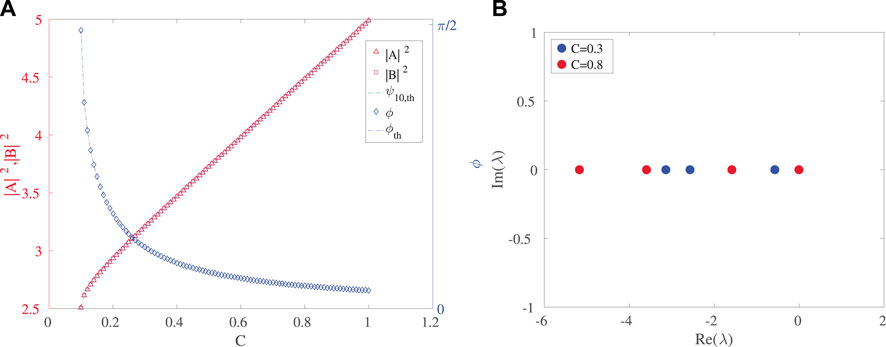
FIGURE 1. (A) Amplitude and phase of steady state symmetric solutions from the upper symmetric branch. (B) Spectral plane (Re(λ),Im(λ)) representation of the eigenvalues λ for C = 0.3 and C = 0.8. Other parameter values are γ = 1.0, δ = 0.1, g₁ = 0.3, g₂ = 0.4 and $\tilde{g}=0.5$. In the left panel, the left axis corresponds to amplitudes, while the right to phases, while the subscript “th” corresponds to the theoretical prediction and the symbols correspond to numerical results.

FIGURE 2

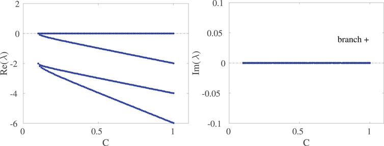
FIGURE 2. Dependence of the real and imaginary parts of the eigenvalues of steady state symmetric solutions from the upper (+) branch. The other parameter values remain as in the caption of Figure 1.

Figure 2 shows the real and imaginary parts of the eigenvalues as a function of C. Given that the largest value of the real part is zero, this upper branch is spectrally stable. That is, all the relevant eigendirections are associated with decay, aside from a neutral one (associated with an overall phase freedom). Recall that this is a non-conservative system, hence the relevant eigenvalues have to be in the left-half of the spectral plane (or on the imaginary axis thereof) for stability, as is the case for this branch. Indeed, we will see below that this is the only spectrally stable branch of this nonlinear anti-$\mathcal{PT}$-symmetric dimer.

In Figures 3, 4 we illustrate the corresponding results for the “negative sign” solution in Eq. 11, i.e., the hereafter termed lower branch. This time the amplitude decreases with increasing C, and the phase difference increases from just over π/2 to π. The continuation was started a little above C = δ; for C = δ we would expect both solutions to have ϕ = π/2. It is relevant to also note that the branches of Figures 1–3 coincide at the critical point of C = δ at which the relevant SN bifurcation arises with the upper branch corresponding to the node, while the lower one to the saddle. In accordance with this picture the spectra show again a purely real set of eigenvalues and in Figure 4 with one of them being positive and hence corroborating the instability of the saddle (−) symmetric configuration of the lower branch.

FIGURE 3

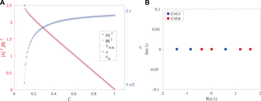
FIGURE 3. (A) Amplitude and phase of steady state symmetric solutions from the lower branch. (B) Spectral plane representation of eigenvalues for C = 0.3 and C = 0.8. The other parameter values are the same as in Figure 1.

FIGURE 4

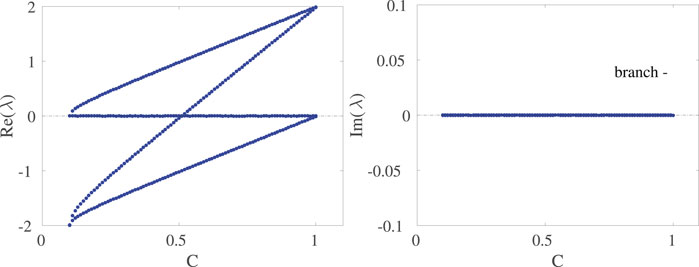
FIGURE 4. Linear spectra of steady state symmetric solutions from the lower branch. Importantly, in addition to the instability starting at the saddle-node bifurcation which gives rise to its existence, the solution inherits an additional instability at a bifurcation point of C = 0.51. The rest of the parameters are the same as in the previous Figures.

This is confirmed systematically also in Figure 4, where the relevant unstable eigenvalue is seen to grow from 0 beyond the bifurcation point. Interestingly, an additional unstable eigendirection arises at some intermediate value of C as well, rendering the relevant branch more unstable. We will return to the latter more elaborate bifurcation shortly. Nevertheless, for the interval of values of C considered, the former instability is always stronger (i.e., has a higher growth rate) than the latter one.

Now we turn to the results obtained for the two branches of asymmetric solutions. Here, the bifurcation picture is far more elaborate. The bifurcation diagram as a function of the parameter C is shown in Figure 5. Let us note that in this diagram the symmetric (node upper and saddle lower) branches are also shown and their SN bifurcations are shown via the green (solid) curves, while the asymmetric branches are shown with blue (dashed) lines. The main feature of the latter is that there is a 3-way collision between the 2 asymmetric branches and the lower symmetric one, close to $C_{cr}^{(1)}=0.51$. This is easily seen in the detailed (right) panel for the amplitude dependence. The upper asymmetric branch goes past a fold en route to that collision, existing as a solution up to $C_{cr}^{(2)}=0.5128$. Indeed, the latter point is associated with a SN bifurcation corresponding to the termination (in terms of values of C) of the upper asymmetric branch. That is, the relevant branch does not exist for higher C values. Interestingly, the algebraic picture is somewhat more complicated in that when solving Eq. 22, the upper branch goes past the turning point of $C_{cr}^{(2)}$ and upon turning around collides with the lower branch $C_{cr}^{(1)}$. Nevertheless, this is, in a sense, an “artifact” of the closed form formulae of the analytical solutions of Eq. 22. Observing the curves in the bifurcation diagram of Figure 5, one can see that the “inner” curves (the ones closer to the green line before $C_{cr}^{(1)}=0.51$ at this critical point) collide between them and therefore become instantaneously symmetric before smoothly continuing en route to the collision with the “outer” (top and bottom) curves at $C_{cr}^{(2)}=0.5128$. That is to say, the former critical point signals a transcritical bifurcation, between the asymmetric and the symmetric branch, while the latter critical point signals a SN bifurcation leading to the termination of asymmetric branches.

FIGURE 5

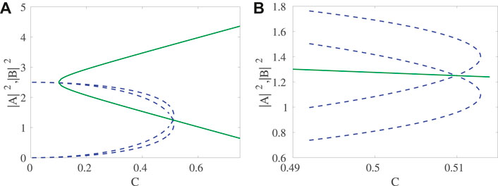
FIGURE 5. Bifurcation diagram as a function of (control) parameter C. (A) amplitudes |A|², |B|²; (B) zoom in for the region where bifurcations occur. We do not show here the results for ϕ and ξ, although the same bifurcation features can be observed therein. The solid (green) lines pertain to the symmetric branches of solutions, while the dashed (blue) ones to the asymmetric branches.

Indeed, this picture is corroborated by the relevant eigenvalue plots. Figure 6 illustrates some prototypical examples of the spectral plane of the upper and lower asymmetric solutions. Both of them bear a complex eigenvalue pair (i.e., are associated with an oscillatory instability featuring both growth and oscillation, as we will also see below). However, in the case of the upper branch this instability is persistent up to C ≈ 0.430, while in the lower branch, it splits into two real eigenvalues earlier (parametrically), i.e., for C ≈ 0.287. Notice, accordingly, the difference for the red points of C = 0.4 in the right panel of Figure 6.

FIGURE 6

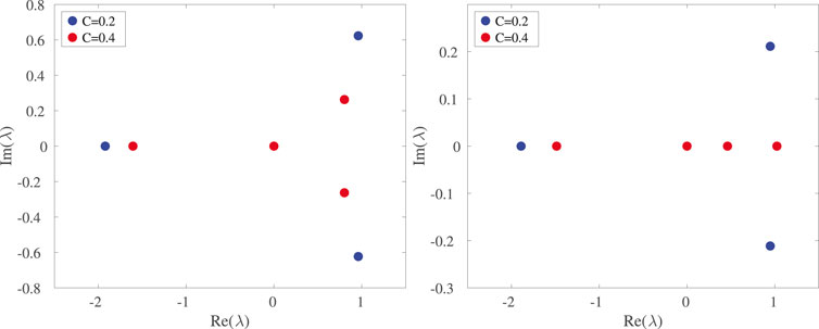
FIGURE 6. (A,B) Spectral plane representation of eigenvalues for C = 0.2 and C = 0.4 for the upper (left panel) and lower (right panel) asymmetric branches. The rest of the parameters are the same as in the previous figures.

The conversion of these complex pairs into real ones is also manifest explicitly in the top panels of the detailed Figure 7, which constitutes a central set of our numerical findings. Indeed, the top right panel shows how the complex pairs collide at the above critical points, thereafter splitting into two real eigenvalues for the respective branches, as shown in the top left panel of Figure 7. The left panel, admittedly, becomes rather complicated as we approach the critical points $C_{cr}^{(1)}$ and $C_{cr}^{(2)}$ although a collision with the green (lower symmetric) branch is apparent. To that effect, we provide further details in the middle and bottom row panels of this Figure, where the detail of each of the relevant eigenvalues is shown in the vicinity of $C_{cr}^{(1)}$ and $C_{cr}^{(2)}$, i.e., close to the transcritical and the SN bifurcation points, respectively. The “collision” of the asymmetric lower and symmetric branch is evident in these three panels at $C_{cr}^{(1)}$. Especially telling within the right panel of the middle row is the exchange of stability between the symmetric (lower) green branch and the asymmetric branch. Notice that both branches already bear a positive real eigenvalue (hence are unstable). However, the asymmetric branch has a second eigenvalue crossing from positive to negative, while the symmetric one goes in the opposite direction, with the two exchanging their stability in the aforementioned transcritical bifurcation event. Lastly, the asymmetric branch terminates at $C_{cr}^{(2)}$ through a SN bifurcation featured in the middle right panel through two eigenvalues colliding at 0. We believe that this description offers a comprehensive understanding of the bifurcation phenomenology present in the system.

FIGURE 7

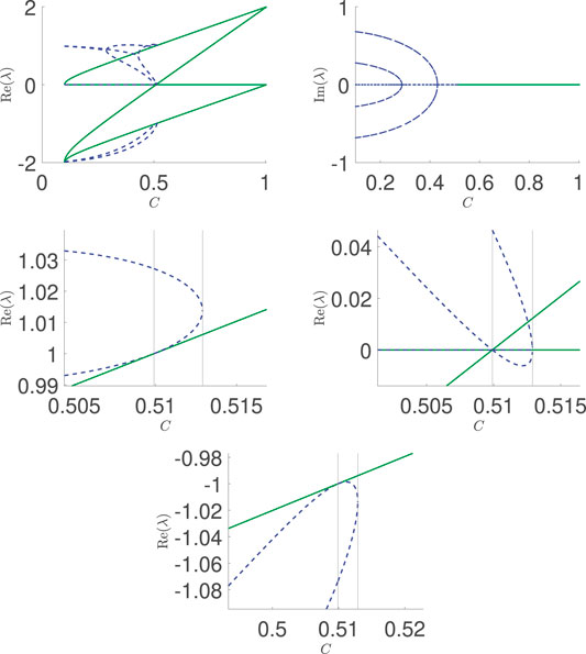
FIGURE 7. Eigenvalues of the asymmetric (and lower symmetric) branches as a function of (control) parameter C. Top left: real part; top right: imaginary part. The second and third row show details of the individual eigenvalues in the vicinity of the bifurcation points $C_{cr}^{(1)}=0.51$ (transcritical) and $C_{cr}^{(2)}=0.5128$ (SN), marked by thin black lines. Once again green (solid) lines are used for the lower symmetric branch, while dashed (blue) ones for the asymmetric branches. See the text for further discussion.

5.1 Dynamics

Guided by the stability results we evolved initial conditions of both branches and both types of solutions for C values that should illustrate some of the principal features of the stability diagrams picture. In the case of the symmetric, upper branch we verified that initiating the dynamics along this branch yields a perfectly stable dynamical evolution, even upon perturbation of the branch (results not shown for brevity). On the other hand, the initial conditions belonging to the lower symmetric branch evolve towards the upper branch, as may be expected, given that for both C = 0.3 and C = 0.7 it has an eigenvalue with a positive real part and the only stable solution of the system is the upper symmetric one. This is shown in the top panels of Figure 8.

FIGURE 8

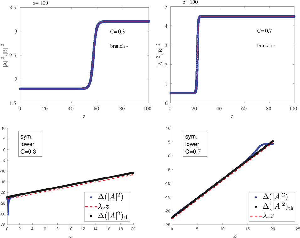
FIGURE 8. Evolution of symmetric steady state solutions from the lower branch in linear (top) and semilog (bottom) scale. The left panels are for C = 0.30 and right ones for C = 0.70. Other parameter values as in previous figures. It is clear (from the top panels) that the evolution tends to the stable symmetric (upper branch) structures. In the bottom panels, the difference of the amplitude from the steady state amplitude is shown, numerically (blue dots), and semi-analytically via the prediction of the linear stability analysis (black dots with subscript th). The growth of the exponential instability (linear in the semilog plot) based on the dominant eigenvalue is shown by the red dashed line. See also the discussion in the text.

To illustrate the relevant instability more clearly (and its connection with the spectral picture that we have previously obtained), we perturb the initial condition (steady state) with the eigenvector corresponding to the eigenvalue with the largest real part, in order to accelerate the decay and to check if the evolution corresponds indeed to the growth at a rate associated with the real part of the eigenvalue, λ_r,max (the maximal positive real eigenvalue). We present these results for the lower branch, both for C = 0.30 and for C = 0.70 in the lower panel of Figure 8. We plot the semilog of the variation in power relative to the steady state (subscript ss) solution, $\log \left(|A(z){|}^2-|A_{ss}{|}^2\right)$. As evidenced in the figure, the growth slope matches very accurately the real part of the (most unstable) eigenvalue, confirming the results of our spectral analysis.

Now let us look at the dynamics of the asymmetric solutions, both for the upper and lower branch, illustrated in Figures 9, 10, respectively. As predicted by linear stability, in both cases it is perceivable that the initial state evolves towards a symmetric state, and from the final amplitude it is the upper symmetric state, i.e., the only linearly stable configuration available in the system. This is shown in the linear scale plots of the top panels. On the other hand, we also present the semilog plots of the evolution of the departure from initial steady state. In this case we also represent the theoretical curve for the prediction for the evolution of the perturbation along the eigenvector with largest real part; this curve is denoted $\mathrm{\Delta }{(|A{|}^2)}_{\text{th}}$. Similar to the (lower branch) symmetric case, the plot of Δ(|A|²) = log(|A(z)|² − |A_ss|²) in Figures 9, 10 shows a relation to the eigenvalue, as the slope of the tangent to the curve. However, in this case, the relevant eigenvalues are complex, hence there is not only a growth associated with the real part of the eigenvalues, but also an oscillation associated with the imaginary part of the pertinent eigenvalue. This oscillation is clearly evident in the bottom panel of both figures, and it indeed matches the expected one on the basis of the imaginary part of the eigenvalue. This definitively corroborates the spectral results of our stability analysis. Recall, however, from Figure 6 that the lower asymmetric branch has a purely real instability for C = 0.4 (while it has a complex pair for C = 0.2). This is also corroborated by the results of Figure 10, by comparing the exponential growth of the former case (right panels) with the oscillatory one of the latter case (left panels).

FIGURE 9

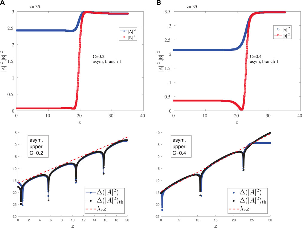
FIGURE 9. Evolution of steady state solutions from the asymmetric upper branch (A) C = 0.2 (B) C = 0.4. The amplitudes of the top panel evolve towards the symmetric values of the upper symmetric (stable) branch in the top panels. The bottom panels show the growth process in semilog scale corroborating not only the real part involving the growth (dashed red line), but also the imaginary part associated with the oscillation (cf. the theoretical curve in black vs. the numerical results in blue).

FIGURE 10

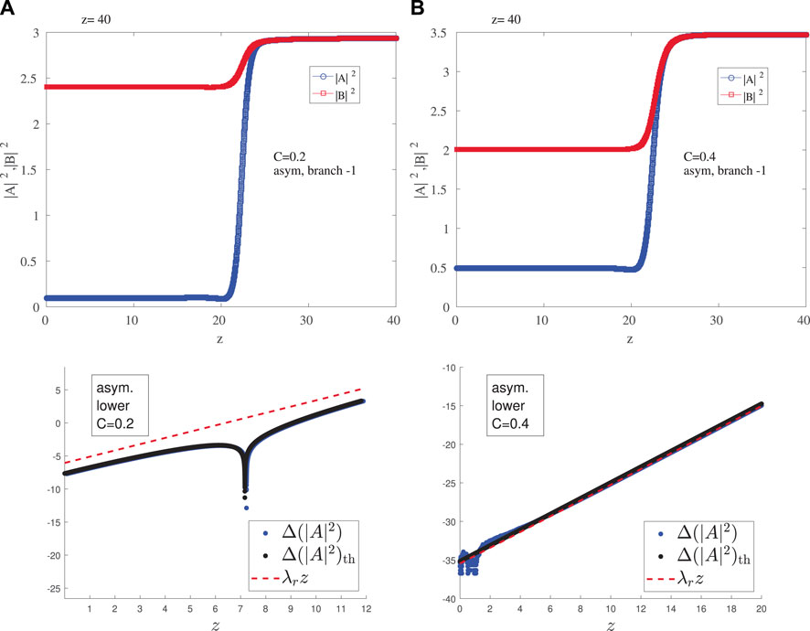
FIGURE 10. Evolution of steady state solutions from the asymmetric lower branch (A) C = 0.2 (B) C = 0.4. See text for other parameter values. The figure is similar to Figure 9, however for this branch the case of C = 0.2 has a complex pair, while that of C = 0.4 possesses only real eigenvalues; cf. Figure 6.

6 Conclusions and Future Work

In the present work, we have explored a nonlinear variant of the anti-$\mathcal{PT}$ symmetric dimer problem. The linear version of this setup has already been explored in a variety of settings, including optical waveguides [23, 24, 31], coupled electrical circuit resonators [26] and atomic vapour cells [25]. Some of these works have already proposed variants of the relevant settings that would involve nonlinearity [25], while for others we argued about the fact that nonlinearity inclusion would be natural on the basis of the nature of the response of such systems at larger amplitudes. We have explored the most prototypical nonlinear dimer setting and were able, given the few-degrees-of-freedom nature of the setting, to obtain solutions analytically for the stationary states of the system. We found, in particular, two symmetric solutions arising via a saddle-node bifurcation and also identified two asymmetric solutions which are involved in a transcritical bifurcation with the lower symmetric branch, as well as in a saddle-node bifurcation leading to the termination of the asymmetric solutions. Out of these four solution branches, only one was found to be spectrally stable and indeed was identified as a generic attractor of the dynamics of the system, even when starting from the unstable symmetric or asymmetric solutions. Our spectral analysis was straightforwardly corroborated via direct numerical simulations of the evolution dynamics which showed the growth along the predicted unstable eigendirections of unstable stationary states with the appropriate rates, and the eventual approach to the sole dynamical attractor of this system, namely the stable (upper) symmetric branch.

Naturally, these results pave the way for numerous further studies of anti-$\mathcal{PT}$ symmetric systems along a similar vein to what was done in the $\mathcal{PT}$-symmetric case [20–22]. In particular, one can examine so-called anti-$\mathcal{PT}$ symmetric oligomers ($\mathcal{PT}$-symmetric ones were explored, e.g., in [12, 17, 18]), as well as lattices of such elements (again, corresponding $\mathcal{PT}$-symmetric explorations could be found in [34, 35]).

Given that the bifurcation picture for the anti-$\mathcal{PT}$ -symmetric dimer is far more complex (and involving multiple bifurcations), as shown herein, in comparison to the corresponding $\mathcal{PT}$-symmetric dimer, it is expected that the situation with anti-$\mathcal{PT}$-symmetric oligomers (trimer, quadrimer, etc.) will be significantly more complex than the regular $\mathcal{PT}$-symmetric ones considered earlier and summarized, e.g., in [20–22]. This is a topic particularly relevant for future studies, and the results/methods proposed herein as well as the differences between the $\mathcal{PT}$ and anti-$\mathcal{PT}$ systems for the dimer could be a useful guide towards such efforts in the near future. These extensions can be considered not only in one- but also in higher dimensions, with the latter implying a different coupling between the nodes constituting the oligomer. Furthermore, here, we have concerned ourselves with cubic Kerr-type nonlinearities, yet some of the above settings seem to be well-suited for different types of nonlinear terms, including four-wave-mixing ones [25], with the latter being another topic worthwhile of further study. Such considerations are currently in progress and will be reported in future publications.

Data Availability Statement

The raw data supporting the conclusion of this article will be made available by the authors, without undue reservation.

Author Contributions

AR: Data curation, Investigation, Software, Validation, Visualization, Writing—original draft; RR: Data curation, Investigation, Software, Validation, Visualization, Writing—original draft; VK: Conceptualization, Methodology, Investigation, Writing—review and editing; AS: Conceptualization, Methodology, Investigation, Writing—review and editing. PK: Conceptualization, Methodology, Investigation, Validation, Supervision, Writing—original draft.

Funding

AR acknowledges financial support from FCT-Portugal through Grant No. UIDB/04650/2020. This material is based upon work supported by the US National Science Foundation under Grants No. PHY-2110030 and DMS-1809074 (PK). VK acknowledges financial support from the Portuguese Foundation for Science and Technology (FCT) under Contract no. UIDB/00618/2020. The work of AS at Los Alamos National Laboratory was carried out under the auspices of the U.S. DOE and NNSA under Contract No. DEAC52-06NA25396 and supported by U.S. DOE.

Conflict of Interest

The authors declare that the research was conducted in the absence of any commercial or financial relationships that could be construed as a potential conflict of interest.

Publisher’s Note

All claims expressed in this article are solely those of the authors and do not necessarily represent those of their affiliated organizations, or those of the publisher, the editors and the reviewers. Any product that may be evaluated in this article, or claim that may be made by its manufacturer, is not guaranteed or endorsed by the publisher.

References

1. Bender CM, Boettcher S. Real Spectra in Non-hermitian Hamiltonians Having PT Symmetry. Phys Rev Lett (1998) 80:5243–6. doi:10.1103/physrevlett.80.5243

CrossRef Full Text | Google Scholar

2. Bender CM, Brody DC, Jones HF. Complex Extension of Quantum Mechanics. Phys Rev Lett (2002) 89:270401. doi:10.1103/physrevlett.89.270401

PubMed Abstract | CrossRef Full Text | Google Scholar

3. Rüter CE, Makris KG, El-Ganainy R, Christodoulides DN, Segev M, Kip D. Observation of Parity-Time Symmetry in Optics. Nat Phys (2010) 6:192–5. doi:10.1038/nphys1515

CrossRef Full Text | Google Scholar

4. Peng B, Özdemir ŞK, Lei F, Monifi F, Gianfreda M, Long GL, et al. Parity-Time-Symmetric Whispering-Gallery Microcavities. Nat Phys (2014) 10:394–8. doi:10.1038/nphys2927

CrossRef Full Text | Google Scholar

5. Peng B, Özdemir ŞK, Rotter S, Yilmaz H, Liertzer M, Monifi F, et al. Loss-Induced Suppression and Revival of Lasing. Science (2014) 346:328–32. doi:10.1126/science.1258004

PubMed Abstract | CrossRef Full Text | Google Scholar

6. Wimmer M, Regensburger A, Miri M-A, Bersch C, Christodoulides DN, Peschel U. Observation of Optical Solitons in $PT$-Symmetric Lattices. Nat Commun (2015) 6:7782. doi:10.1038/ncomms8782

PubMed Abstract | CrossRef Full Text | Google Scholar

7. Schindler J, Li A, Zheng MC, Ellis FM, Kottos T. Experimental Study of Active LRC Circuits with PT Symmetries. Phys Rev A (2011) 84:040101. doi:10.1103/physreva.84.040101

CrossRef Full Text | Google Scholar

8. Schindler J, Lin Z, Lee JM, Ramezani H, Ellis FM, Kottos T. $PT$-Symmetric Electronics. J Phys A: Math Theor (2012) 45:444029. doi:10.1088/1751-8113/45/44/444029

CrossRef Full Text | Google Scholar

9. Bender N, Factor S, Bodyfelt JD, Ramezani H, Christodoulides DN, Ellis FM, et al. Observation of Asymmetric Transport in Structures with Active Nonlinearities. Phys Rev Lett (2013) 110:234101. doi:10.1103/physrevlett.110.234101

PubMed Abstract | CrossRef Full Text | Google Scholar

10. Bender CM, Berntson BK, Parker D, Samuel E. Observation of PT Phase Transition in a Simple Mechanical System. Am J Phys (2013) 81:173–9. doi:10.1119/1.4789549

CrossRef Full Text | Google Scholar

11. Ramezani H, Kottos T, El-Ganainy R, Christodoulides DN. Unidirectional Nonlinear $PT$-Symmetric Optical Structures. Phys Rev A (2010) 82:043803. doi:10.1103/physreva.82.043803

CrossRef Full Text | Google Scholar

12. Li K, Kevrekidis PG. $PT$-Symmetric Oligomers: Analytical Solutions, Linear Stability, and Nonlinear Dynamics. Phys Rev E (2011) 83:066608. doi:10.1103/physreve.83.066608

PubMed Abstract | CrossRef Full Text | Google Scholar

13. Rodrigues AS, Li K, Achilleos V, Kevrekidis PG, Frantzeskakis DJ, Bender CM. $PT$-Symmetric Double-Well Potentials Revisited: Bifurcations, Stability and Dynamics. Rom Rep Phys (2013) 65:5.

Google Scholar

14. Sukhorukov AA, Xu Z, Kivshar YS. Nonlinear Suppression of Time Reversals in PT-Symmetric Optical Couplers. Phys Rev A (2010) 82:043818. doi:10.1103/physreva.82.043818

CrossRef Full Text | Google Scholar

15. Xu H, Kevrekidis PG, Saxena A. Generalized Dimers and Their Stokes-Variable Dynamics. J Phys A: Math Theor (2015) 48:055101. doi:10.1088/1751-8113/48/5/055101

CrossRef Full Text | Google Scholar

16. Barashenkov IV, Pelinovsky DE, Dubard P. Dimer with Gain and Loss: Integrability and $PT$-Symmetry Restoration. J Phys A: Math Theor (2015) 48:325201. doi:10.1088/1751-8113/48/32/325201

CrossRef Full Text | Google Scholar

17. Li K, Kevrekidis PG, Malomed BA, Günther U. Nonlinear $PT$-Symmetric Plaquettes. J Phys A: Math Theor (2012) 45:444021. doi:10.1088/1751-8113/45/44/444021

CrossRef Full Text | Google Scholar

18. Zezyulin DA, Konotop VV. Nonlinear Modes in Finite-Dimensional PT-Symmetric Systems. Phys Rev Lett (2012) 108:213906. doi:10.1103/physrevlett.108.213906

PubMed Abstract | CrossRef Full Text | Google Scholar

19. Gupta SK, Deka JP, Sarma AK. Nonlinear Parity-Time Symmetric Closed-Form Optical Quadrimer Waveguides: Attractor Perspective. Eur Phys J D (2015) 69:199. doi:10.1140/epjd/e2015-60034-7

CrossRef Full Text | Google Scholar

20. Suchkov SV, Sukhorukov AA, Huang J, Dmitriev SV, Lee C, Kivshar YS. Nonlinear Switching and Solitons in PT‐Symmetric Photonic Systems. Laser Photon Rev (2016) 10:177–213. doi:10.1002/lpor.201500227

CrossRef Full Text | Google Scholar

21. Konotop VV, Yang J, Zezyulin DA. Nonlinear Waves in $PT$-Symmetric Systems. Rev Mod Phys (2016) 88:035002. doi:10.1103/revmodphys.88.035002

CrossRef Full Text | Google Scholar

22. Christodoulides D, Yang J. Parity-Time Symmetry and its Applications. Singapore: Springer Nature (2018).

Google Scholar

23. Ge L, Türeci HE. Antisymmetric $PT$-Photonic Structures with Balanced Positive- and Negative-Index Materials. Phys Rev A (2013) 88:053810. doi:10.1103/physreva.88.053810

CrossRef Full Text | Google Scholar

24. Yang F, Liu Y-C, You L. Anti $PT$-Symmetry in Dissipatively Coupled Optical Systems. Phys Rev A (2017) 96:053845. doi:10.1103/physreva.96.053845

CrossRef Full Text | Google Scholar

25. Peng P, Cao W, Shen C, Qu W, Wen J, Jiang L, et al. Anti-Parity-Time Symmetry with Flying Atoms. Nat Phys (2016) 12:1139–45. doi:10.1038/nphys3842

CrossRef Full Text | Google Scholar

26. Choi Y, Hahn C, Yoon JW, Song SH. Observation of an Anti-PT-Symmetric Exceptional point and Energy-Difference Conserving Dynamics in Electrical Circuit Resonators. Nat Commun (2018) 9:2182. doi:10.1038/s41467-018-04690-y

PubMed Abstract | CrossRef Full Text | Google Scholar

27. Cen J, Saxena A. Anti $PT$-Symmetric Qubit: Decoherence and Entanglement Entropy. Phys Rev A (2022) 105:022404. doi:10.1103/physreva.105.022404

CrossRef Full Text | Google Scholar

28. Konotop VV, Zezyulin DA. Odd-Time Reversal PT Symmetry Induced by an Anti-PT-Symmetric Medium. Phys Rev Lett (2018) 120:123902. doi:10.1103/physrevlett.120.123902

PubMed Abstract | CrossRef Full Text | Google Scholar

29. Hang C, Zezyulin DA, Huang G, Konotop VV. Nonlinear Topological Edge States in a Non-Hermitian Array of Optical Waveguides Embedded in an Atomic Gas. Phys Rev A (2021) 103:L040202. doi:10.1103/physreva.103.l040202

CrossRef Full Text | Google Scholar

30. Li Q, Zhang C-J, Cheng Z-D, Liu W-Z, Wang J-F, Yan F-F, et al. Experimental Simulation of Anti-Parity-Time Symmetric Lorentz Dynamics. Optica (2019) 6:67. doi:10.1364/optica.6.000067

CrossRef Full Text | Google Scholar

31. Ge L, Wang W. In: PG Kevrekidis, J Cuevas-Maraver, and A Saxena, editors. Emerging Frontiers in Nonlinear Science. Cham: Springer International Publishing (2020).

Google Scholar

32. Remoissenet M. Waves Called Solitons. Berlin: Springer-Verlag (1993).

Google Scholar

33. Alexeeva NV, Barashenkov IV, Rayanov K, Flach S. Actively Coupled Optical Waveguides. Phys Rev A (2014) 89:013848. doi:10.1103/physreva.89.013848

CrossRef Full Text | Google Scholar

34. Kevrekidis PG, Pelinovsky DE, Tyugin DY. Nonlinear Dynamics in PT-Symmetric Lattices. J Phys A: Math Theor (2013) 46:365201. doi:10.1088/1751-8113/46/36/365201

CrossRef Full Text | Google Scholar

35. Kevrekidis PG, Pelinovsky DE, Tyugin D. Nonlinear Stationary States in PT-Symmetric Lattices. SIAM J Appl Dyn Syst (2013) 12:1210–36. doi:10.1137/130912694

CrossRef Full Text | Google Scholar