A Ubiquitous Collective Tragedy in Transport

1 Introduction

Despite the possibility of new technical solutions being developed to reduce the impact of an ever-increasing population on our climate, there is still a need for radical social transformation to ensure sustainability. Systems formed by unregulated and disorganised individuals often fail due to their competitive, over-exploitation of a shared resource or the inadvertent costs that each person puts on society, leading to a collective tragedy. The tragedy of the commons can be described as a situation in which the members of a group act solely in their self-interest, trying to maximise their own outcome or benefit, but resulting in the unintended consequence of the deterioration of a wider social outcome [1, 2]. This type of tragedy has been observed in nature, for example, in territorial conflicts between animals, plant competition for light and even high virulence in parasites [3]. In social terms, aspects such as pollution, climate change, or the super rich’s wealth concentration can all be posed in terms of a tragedy, where individual action tends to pollute more and concentrate more wealth [4].

Road traffic can also be thought of as a tragedy [5]. For example, increasing road capacity in response to congested conditions can make congestion even worse since some people switch from some other mode of transport to using a car [6, 7]. Also, it has been noted that selfish routing considerably increases the time lost to congestion [8]. Moreover, it has recently been shown that a collective decision could lead to the worst-case scenario in mode choice, whereby people choose to drive, as it is their fastest method, but this takes the city to the highest average commuting time as well as increasing pollution [9]. If everyone minimises their commuting time, this could result in maximum congestion for everyone. Individual action might lead to a tragedy where the outcomes are far from sustainable cities.

People often choose their transport mode taking many factors into account, including cost, the risk involved, accessibility, levels of comfort and other personal preferences, but the time of a journey is often the key factor, especially for daily commutes [6, 10–18]. People tend to choose the fastest method and, in many cases, commuting by car is faster than travelling by public transport, cycling or walking. However, car drivers impose themselves on the traffic, that is, they increase the commuting time of others and the whole city. And a similar effect happens for other transport modes, where more users impose costs on others, although the congestion effects are smaller compared to the congestion caused by drivers. Perhaps cyclists struggle to find a parking spot with too many cyclists, or walking down a busy street is slowed down by other pedestrians. It has been argued that public transport might undergo a virtuous cycle, where more users will induce the operator to increase their service frequency, decreasing waiting times and hence attracting even more users [19–22]. There is, however, a limit to how virtuous the cycle of public transport might be. Metro lines have a limit to the number of trains they can accommodate, so their capacity cannot expand beyond a certain limit. Access time is a large proportion of the door-to-door travel time for public transport [6] which tends to increase with more users. Stations have finite space. Cities around the world experience a saturated public transport during rush hour with queues for buying a ticket, longer alighting times, the need to let some services go, which are full, or having to travel in uncomfortable conditions [23–25].

Besides the congestion on the roads, there are other negative impacts that cars put on cities, such as the need for more infrastructure and an increase in the demand for parking space, pollution related to both the production and combustion of fuel, to name but a few [26]. Cities do not have enough road space for everyone who wishes to travel by car [27]. However, road users do not usually take into account the costs they inflict on others [28, 29]. Cities are facing a severe challenge to remain sustainable, and Metropolitan councils make great efforts to promote walking, cycling, and the use of public transport rather than driving [11, 30–34]. However, the system has memory in terms of the built environment. Many cities have invested considerable funds to construct car infrastructure, leading to an expansion of urban sprawl. This spending also means that there is a lack of budget to fund alternative projects, so decreasing the chances that a person will ever use public or other modes of transport [35, 36], making it very difficult to change commuting behaviour [37].

The traffic in a city and the number of users of a transportation mode are the results of the decisions made by millions of people every day. If we regard individuals as being rational, in the sense that their choices aim to minimise their commuting time (or cost) [38–41], then the resulting traffic and modal share are the consequences of these decisions [11, 42]. However, the commuting choice of a person necessarily impacts the rest of the travellers. Transport supply, given by the capacities of the roads, transit system, bicycle lanes and pavement, etc., is fixed for relatively long periods. Furthermore, there is competition between modal shares since they share parts of the urban space. This is mainly noticed by the increase in the travel time that extra users impose on the rest of the travellers, for example, in the reduction of comfort that an additional transit user implies for the rest of the passengers in a bus, or the reduction of safety that an extra motorist imposes on pedestrians, cyclists and other motorists. This implies that an individual’s choice of transportation mode depends on the choices of the rest of the travellers, through the cost that they induce on each of the travel modes.

There is a complex feedback between the choices that travellers make and the state of the transportation network, as travellers seek to minimise their commuting time, but the outcome depends on the choices of all other travellers. Furthermore, traffic, seen as a game, is a non-cooperative system, so people only care about their own commuting time. We say that a system is in equilibrium when no “player” (user or commuter) can further minimise their commuting time by unilaterally changing their transportation mode, and if on the contrary, they change it, then they experience a higher commuting time [43–45]. Thus, an equilibrium is observed when the commuting time for all used transport modes is the same [28, 46, 47]. In idealised scenarios, such as laboratory decision experiments, it has been found that equilibrium is reached after repeated choices of participants [48, 49].

If the choice of the mode of transportation depends solely on the perceived length of commuting time incurred by the decision-maker (without considering the cost induced to the rest of the travellers), then the equilibrium will not match the social optimum [50]. Thus, it is often regarded as selfish behaviour. This means that the social cost at equilibrium might be greater than the minimum social cost. Therefore, we are in a tragic situation, in which the efficiency of a system degrades due to selfish behaviour [51, 52]. The decrease in social efficiency of a system is often referred to as the price of anarchy [53], defined as a quantitative measure between the worst possible equilibrium and the social optimum. In the context of route choice, the price of anarchy has been estimated to be up to 33%, meaning that drivers may spend up to one third more of their time in congestion by not behaving cooperatively [54–56].

Here, we model the collective evolution of a modal share in a city, where some individuals switch between distinct modes, favouring faster methods of transport [9, 11]. Selecting the modal share is conceived as an iterative, multiplayer non-cooperative game [57]. A collective dynamical system is considered, where faster methods become more popular. Assuming a constant baseline commuting time and an increasing linear function for the induced times for travel of each mode of transport, we show that a unique equilibrium exists and that it forms an attractor node in the system, meaning that the city will eventually reach that equilibrium for all initial internal conditions (where all modes begin with at least one user). We then construct the city “trajectories,” that is, the sequence of changes in modal shares over time. We classify a modal share as “tragic” if the average commuting time of the city increases with time at some stage in the trajectory. Except for one scenario, where all baselines and direct costs are equal, there are always tragic trajectories. It is possible to find a modal share where users switching to a faster mode of transportation results in a slower system overall. The set of modal shares where trajectories are tragic is not empty, and indeed there may be a substantial tragic region. Even when all switches minimise the individual commuting time, a city might become slower as a result. Further, we show that a novel transport method might become popular if its baseline commuting time is small, but the collective outcome of introducing a novel mode might be tragic if the direct costs are high (so, the novel mode becomes less efficient) and if it has high induced costs (so, it makes other modes less efficient as well). Thus, we show that some novel technology might create a costly and undesired collective system.

2 Results

2.1 Changing Between Transport Modes

Commuting is, in general, not an enjoyable activity [58] and each journey has some degree of “undesirability” [6, 46]. This undesirability, or cost, varies from person to person and across transport methods [59]. For example, waiting time is particularly important in public transport since users view it as more burdensome than the same amount of time spent travelling [60]. Here, we assume that any undesirability of a journey can be measured, compared across users and expressed as the minutes that the journey takes.

Every person in a city elects a mode of transport from a pool of κ transport modes. Consider a city with N (fixed) individuals who, at time t, choose to commute using a particular mode of transportation. Let x_i(t) be the number of users of mode i at time t, with i = 1, 2, … , κ. Since everyone picks a mode of transportation, then we only consider points inside the simplex X_N = {x | ∑_ix_i = N}. We assume that the level-of-service of a mode of transportation can be measured in travel time and, thus, all costs can be expressed in commuting minutes of an average journey for each transport mode [9]. The commuting time of each transport mode is divided into three components: 1) a baseline commuting time, which represents the free-flow travel time, i.e., the commuting time as if the city were “empty,” and two variable costs, representing the additional time due to congestion, that depend on 2) the number of users in the same mode of transportation and 3) the number of users in the other modes. If the modal share, i.e., the distribution of users over different modes at time t, is given by the vector x(t) = (x₁(t), x₂(t), …, x_κ(t)), then the cost of using mode i can be expressed in minutes as

$C_i\left(\mathbf{x}\right)=B_i+D_i\left(\mathbf{x}\right)+I_i\left(\mathbf{x}\right),(1)$

where B_i is a constant baseline commuting time for mode i, the function D_i is the direct cost that users of i impose to the users on the same mode i, and I_i are the indirect costs imposed by the users of other transport modes. In general, D_i ≥ 0 and, if the rate of change of D_i with respect to x is denoted by $D_i^{\prime }$, then we assume that $D_i^{\prime }\ge 0$ so that costs are non-negative and do not decrease with more users. Similarly with I_i, so more users of any other mode impose higher indirect costs.

The induced and direct costs are not linear and a variety of functions have been proposed to link travel times and traffic flow [61–63]. For example, the Bureau of Public Roads function was developed by fitting speeds on freeways and it captures a steep increase in travel times with high levels of traffic [63–65]. At a city level, measuring travel time is more complicated. Speed rises with distance from the city centre [6] but also, it has been suggested that the average modal journey time per day and per person has remained constant for decades [59], perhaps due to a polycentric transition of cities [66]. However, although we observe a process that is non-linear at a microscopic level, we assume linear costs at a macroscopic level to simplify our model. Assuming that the induced costs functions are linear, we can express the commuting time for all transport modes as

$\mathbf{C}\left(\mathbf{x}\right)=\mathbf{B}+\mathcal{M}\mathbf{x},(2)$

where C(x) is the commuting time vector (a function), B are the fixed baseline commuting times and $\mathcal{M}$ is a matrix with the arranged marginal costs (with the direct costs on the diagonal).

In general, more car users imply a higher commuting time for driving, even if that means fewer cyclists or walkers, and similarly for other modes of transport. Thus, we assume that each entry of $\mathcal{M}$ are non-negative, and in general, the direct costs are higher than the induced costs of other modes, so the elements in the diagonal will be the largest values of each row.

We assume that there is some modal share for all transport modes for which the commuting time is lower than other transport modes. That is, if there are enough walkers, cyclists and drivers, then using public transport becomes faster. With enough drivers and public transport users, then walking is faster and so on. Under such conditions, no commuting mode is dominant, i.e., no transportation mode is faster than the others for all modal shares x. Rather, for some modal shares, different transport modes compete with others. If everyone uses a car, it will be the worst (slowest) commuting method. The same applies to public transport, walking and cycling. If everyone uses one transport method, it will be the slowest option due to the imposed costs. Also, there exists an internal point, where the number of users of all transport modes is greater than zero, x°, such that C_i(x°) = C_j(x°), for all pairs i ≠ j, with i, j = 1, 2, … , κ, meaning that there is some internal point for which all commuting methods take the same travel time.

For modal share x, the average commuting time of a trip is given by μ(x) = (1/N)x^⊤C(x), i.e., the commuting time of each mode weighted by its share of users. We can write the average commuting time function as

$\mu \left(\mathbf{x}\right)=\frac{1}{N}\left[{\mathbf{x}}^{\top }\mathbf{B}+{\mathbf{x}}^{\top }\mathcal{M}\mathbf{x}\right].(3)$

The function μ(x) is a paraboloid. It has higher values (commuting times) in $\mu (N,0,\dots ,0)=B_1+{\mathcal{M}}_{11}N$, which is a local maximum (and similarly for μ(0, N, … , 0), and for other modes of transport μ(0, 0, … , N, 0, … , 0)). Thus, there is some modal share, x^*, for which the average commuting time is minimum. That is, μ(x) has some global minimum, μ^* = μ(x^*) for modal share x^*.

2.2 A Dynamical System for Modal Share

Shorter travel times is one of the key factors that make a transport mode more attractive [10, 11, 15, 16, 67]. People often try different commuting options, particularly if others manage to commute faster using a different mode [9]. If cycling, for example, is much faster than using a car, then some drivers might try to commute by bicycle and then make it a habit. Similarly, if the public transport is too slow, people might try other methods and choose a faster option. Users switching becomes a dynamic process at a collective level. More people attracted by the benefits of cycling means higher direct costs, less cycling space, and so slower times for cyclists and fewer costs for drivers or public transport users. More car drivers mean more congestion, and more public transport users lead to more delays, queues, etc. Choosing a transport mode can be thought of as an iterative, multiplayer, evolutionary and non-cooperative game [68, 69]. The strategies are the mode of transportation that each person chooses each day, and their outcome is the commuting time. At each iteration, here taken to be a day, some players switch between the distinct transport alternatives to achieve a faster commute. Users switching between methods alter the modal distribution and the commuting time for all users as a result. A common way in which such types of evolutionary games are modelled is through the so-called replicator equation. The core aspect of the model is that users copy better strategies [70].

Each traveller (or player) chooses their transport method (or strategy) and experiences some commuting time (obtains a payoff, or some “gain” according to the strategy). This results in a dynamical process, where the rate of change of a modal share is given by

$\dot{{\mathbf{x}}_i}=\rho {\mathbf{x}}_i\left(\mu \left(\mathbf{x}\right)-{\mathbf{C}}_i\right),(4)$

where ρ > 0 is a speed parameter, so people switch commuting methods on some time scale. The overdot represents differentiation with respect to time, t. Here, μ(x) − C_i is the difference between the average commuting time and the commuting time for mode i, so that the commuting method i becomes more popular $(\dot{x_i}>0)$ when it is faster than the average.

Equation 4 defines a dynamical behaviour that is frequently used to study the adaptation and co-evolution of biological populations [71–73] possessing some important properties. Firstly, the set X_N = {x | ∑_ix_i = N} is invariant under the dynamics, meaning that a trajectory which begins in X_N, never leaves it [70]. The corners of the set X_N, which are x_i = N and x_j = N for j ≠ i, are fixed points of Equation 4 which might also be termed as an equilibrium. There might also be a fixed point on the edges, where C_i = C_j = μ for any two modes, i and j and x_k = 0 for the others, and there might be a fully internal fixed point x°, where C_i = μ for all modes. Such an internal fixed point, if it exists, forms a Nash equilibrium in the dynamics [74] so that no user wants to change their commuting mode, and if they do, their commuting time is longer (so they or someone else takes the city back to its equilibrium). The corners are not necessarily a Nash equilibrium. Although the corners (or some points along the edge) might form an equilibrium, it is generally unstable to small perturbations. Considering discrete units of time (days, for example) gives a first-order difference equation [75].

2.3 An Equilibrium of Modal Share

A unique internal equilibrium exists (with x_i > 0 for all i = 1, 2, … , κ) if there is a point in X_N such that C_i(x) = C_j(x) for every pair i ≠ j. It is possible to see that, from an arbitrary start, the dynamics will converge to the fixed point x°, hence it becomes asymptotically stable.

For some baseline commuting time B, a cost matrix $\mathcal{M}$ and some initial conditions, x₀, the number of users of each transport mode evolves whilst some are attracted by faster commuting methods. Figure 1 shows plots based on three modes of transport. In the long run, the commuting time of all transport modes converges to the same value if and when an equilibrium is reached.

FIGURE 1

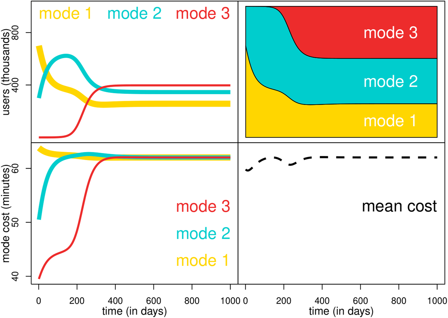
FIGURE 1. Modal share (vertical axis) versus time measured in some dimensionless scale, marked as “days,” so it is a slow process compared to the commutes (horizontal axis) for N = 1, 000, 000 individuals, and some initial distribution, considering three transport modes. The top panels indicates the number of users and their frequency. The bottom panels is the commuting time in minutes for each transport mode and the mean commuting time experienced by all users.

Eventually, users converge to some equilibrium x°, which has the same commuting time for all transport modes (Figure 2). In general, regardless of the initial distribution, all trajectories converge to some equilibrium distribution, although it could be a cyclic behaviour depending on the parameters. With a small value of ρ > 0, the process takes all internal trajectories to some consensual distribution [9]. The rate of convergence depends on the values of ρ, where smaller values take a longer time.

FIGURE 2

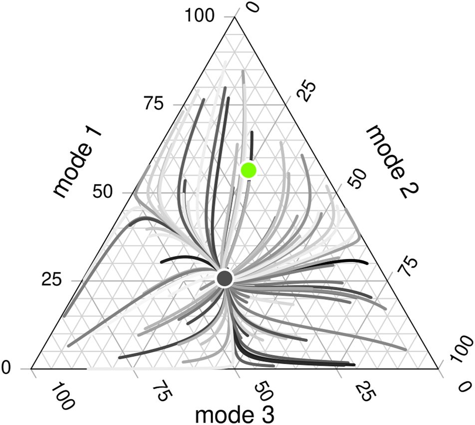
FIGURE 2. Each point in the triangle represents the distribution of users among the three modes of transport. The triangle representation is such that at any point inside the simplex X_N, the number of users of all modes represents the total population. For some point inside the triangle, the amount of users of mode 1 can be identified by following a horizontal line from the left axis. For mode 2, a diagonal line to the lower-left, and for mode 3, a diagonal line to the upper-left. The corners represent modal shares where all users use the same transport system. There is a commuting time associated with each transport mode and an average commuting time for each point. Different trajectories of the modal-share dynamics are observed as curves with different (randomly picked) colours across the simplex. Each curve starts at some randomly picked distribution, and eventually, all curves converge to the same point (the black disc), which is the attractor node and the Nash equilibrium for the dynamics, x°. From all modal shares, there is one configuration which has the lowest average commuting times (the green disc), x^⋆.

If there is a modal share for which each method has the lowest commuting time, that is, if all commuting methods are desirable for some modal share and have the worst commuting time if everyone uses them, then an internal equilibrium exists. See the Methods 4.2 for the details.

2.4 Social Trajectories

The replicator equation is based on the principle that faster commuting methods become more popular since individuals switch to reduce their commuting time. For some initial conditions, x₀, the system produces a trajectory in the space of transport modes X_N. As people switch commuting methods, the collective modal share changes accordingly. Therefore, a trajectory is defined for x(t) as t increases. Also, as time passes, and users switch between commuting methods, the corresponding commuting time for each transport mode changes and the mean commuting time also changes. Combining Equations 4, 3 gives the evolution of the mean commuting time with respect to time

$\frac{d\mu }{dt}=\frac{\rho }{N}\left[B^{\top }+{\mathbf{x}}^{\top }\left(\mathcal{M}+{\mathcal{M}}^{\top }\right)\right]\dot{\mathbf{x}}.(5)$

For different initial conditions x₀, the observed trajectories $\mathbf{x}{(t)}_{{\mathbf{x}}_0}$ and the mean commuting time curve ${\mu }_{{\mathbf{x}}_0}(t)$ are different, although for any internal initial conditions, trajectories will converge to the fixed point x°. Therefore, all mean commuting time curves ${\mu }_{{\mathbf{x}}_0}(t)$ eventually have the same final value μ_x°.

The mean commuting time μ_x varies according to the distribution of users of different transport modes (Figure 3). Equation 3 is a paraboloid in X_N, a function with a single minimum point that increases in all directions. With different values of B and $\mathcal{M}$, the shape of the second-degree polynomial changes and the location of the minimum average commuting time x^* also changes. It is possible to find a point in X_N where the average commuting time is minimum. See the Methods 4.2 for the details.

FIGURE 3

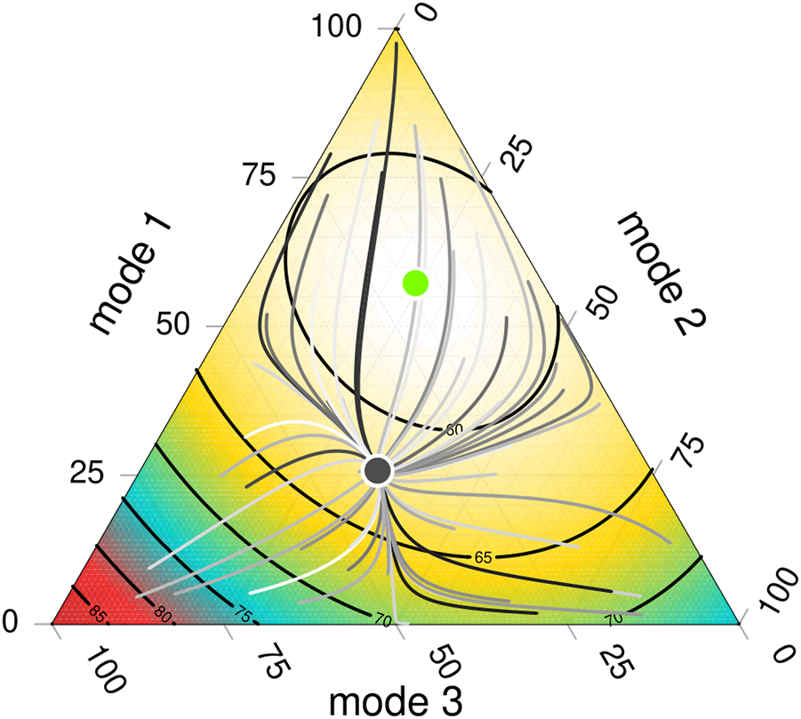
FIGURE 3. The mean commuting time function μ_x gives the weighted time for each transport mode, considering the number of users that experience such commuting times. With linear costs, the function is a second-degree polynomial, with some minimum mean cost which might be inside X_N. Three transport mode options are simultaneously plotted. The black curves marked with numbers 60, 65, 70, and so on, correspond to a contour curve of the commuting time function, where the average commuting times are 60 min, 65 min, etc. The attractor node is the dark disc, and the optimum distribution is the green disc.

The mean commuting time curve ${\mu }_{{\mathbf{x}}_0}(t)$ is a continuous function for t ≥ 0 since it is a trajectory over the domain of a second-degree polynomial. It begins at x₀ and, as time evolves, the trajectory converges to x°.

2.5 Tragedy of the Commons

Each time a person switches from one commuting method to another, they reduce their travelling time. However, as a result of that switching, the average commuting time changes, and it might increase. This scenario happens when higher induced costs imposed on other users compensate for the personal gain from the switching. For example, if a person decides to drive instead of walking, they might save some time by doing this, but the payoff is only for the individual and creates even more traffic for those who already drive. An individual gain becomes a collective loss.

The city’s transport evolves as visualised by trajectories x(t) formed by people trying to decrease their commuting time, although the collective result does not always reduce the mean commuting time. To account for this, here the region where trajectories increase the average commuting times is called tragic. When a city is in a tragic area, the individual action of switching between methods for a faster commute results in a slower collective system, with higher commuting times on average. In the case of only two transport modes, it was observed that the equilibrium, where everyone has minimised their own commuting time, might be reached at a point with the highest mean commuting time for society [9], forming a transport paradox. Here, with the replicator dynamics, it is observed that some trajectories are such that $\dot{\mu }>0$, meaning that the average commuting time increases. For any modal share x, we say that it is tragic if

$\frac{d\mu }{dt}{|}_{\mathbf{x}}>0,(6)$

and we call x to be rewarding if the derivative is not positive. A trajectory might switch between being tragic and rewarding as it moves and evolves in X_N.

In general x° ≠ x^*, so the system will converge to a non-optimum distribution. There is only one scenario where the equilibrium is optimum. If the baseline commuting time is the same for all methods, the direct costs are equal, and the induced costs are the same for all cross mode users, then the stable point is also the minimum mean commuting time. This scenario means that only if the commuting times can be simplified as C_i(x_i) = η + ωx_i, with the same η and ω for all transport methods, then the stable point is optimum. Furthermore, the optimum distribution is x° = x^* = (N/κ, N/κ, … , N/κ) so all methods have the same number of users. See the Methods 4.3 for the details.

Unless x° = x^* (so the equilibrium is the optimum modal share distribution), the modal share of a city converges to a sub-optimum point, where the commuting time for all users is the same but the mean commuting time is higher than the optimum. We can consider the trajectory that begins at the optimum point x^* but eventually converges to x°. It forms a continuous function ${\mu }_{{\mathbf{x}}^{\star }}(t)$ that begins with a lower mean commuting time, but increases for some interval with t > 0. Therefore, except for a unique set of parameters (where x° = x^*), there is always at least one trajectory that begins in the optimum and increases its commuting time as the steps evolve. The tragedy is almost inevitable.

Depending on the initial conditions and the baseline and costs of the transport modes, the system might have many trajectories where average commuting times increase during some periods. Also, some trajectories might switch between being tragic and not being tragic as time evolves (Figure 4).

FIGURE 4

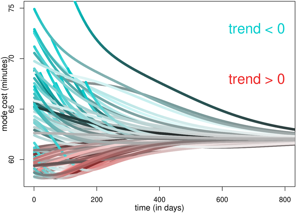
FIGURE 4. Mean commuting time in minutes (vertical axis) for different initial conditions ${\mu }_{{\mathbf{x}}^0}(t)$ as time evolves (horizontal axis) measured in some dimensionless time scale, marked as “days”. All initial conditions converge to the same average commuting time (approximately 62 min). Distinct curves are identified by their shade. When a trajectory increases its commuting time, it is shaded in red, and when it is decreasing its commuting time, it is coloured in blue. Some of the trajectories have, at some point, lower commuting time, but they have some tragic regions where the average commuting time is increasing.

The optimum point x^* might be relatively close to the equilibrium point x°, in which case the price of anarchy is limited. However, the distance between both points might be large, meaning that a city might converge to a modal share that is far from the optimum (Figure 5).

FIGURE 5

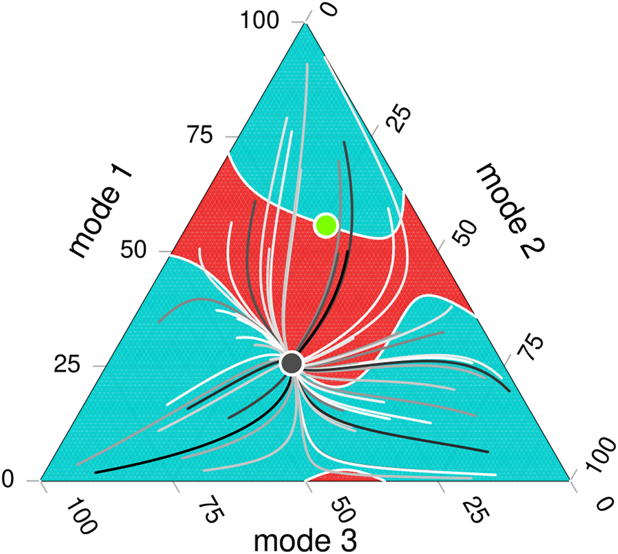
FIGURE 5. Visualisation of the dynamics of the transport system for three different modes showing values of $\frac{d\mu }{dt}$ and some trajectories which converge to the Nash equilibrium of the system. The dark disc is the equilibrium point x°, and the green disc is the minimum commuting time x^⋆. Values where $\frac{d\mu }{dt}<0$ are coloured in blue, such that the dynamics reduce the average commuting times of the city as the dynamic evolves. The red region corresponds to values where $\frac{d\mu }{dt}>0$ in X_N. The red region thus represents the tragedy, where each person is minimising their commuting time but increasing the average. Fifty trajectories with distinct initial conditions are coloured in grey. When a trajectory passes through a red region, it increases its average commuting time.

With different baseline commuting time B and induced and direct costs $\mathcal{M}$, the trajectories are distinct and form different regions with tragedy (Figure 6).

FIGURE 6

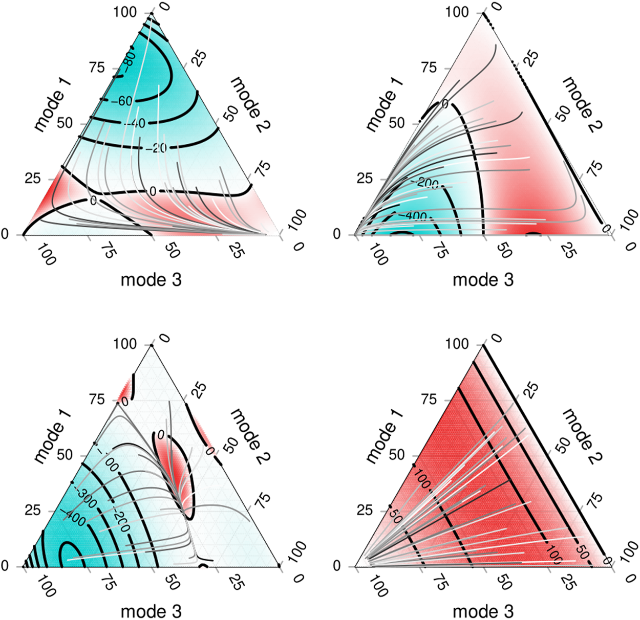
FIGURE 6. Visualisation of the dynamics of the transport system, considering three modes of transport. Each figure shows the result considering different values of $\mathcal{M}$ and of B. The blue areas correspond to trajectories that improve the average commuting time under the replicator dynamics. The red areas correspond to trajectories in the dynamics where individuals change to reduce their commuting time but increase the average commuting time.

The emergent tragedy of the commons can be thought of as the result of a multi-person prisoner’s dilemma [76] where each player picks their best strategy, reducing the collective gain. Playing the iterative game and allowing some players to switch their strategy between one round and the next, our results show that the distribution of users per strategy will converge to some equilibrium, but also, that the collective dilemma imposes a high burden on society. An individual gain results in a collective loss.

2.6 Introducing a New Transport Method and a New Tragedy in the City

Introducing a new technology to a society, even if it offers some gain at first, rather oddly might result in higher commuting times. This result appears to imply that a community would be better if that new technology never existed. For example, contrary to some expectations, it was observed that the introduction of ride-hailing services to compete with more socially desirable modes of transportation, saw trips carried out that otherwise would have been made by public transport or walking [77–80], as well as extra vehicle miles, travelled before each pick-up [81], contributing to growing road congestion and pollution. If the new technology is attractive since it has a small baseline commuting time, then as this becomes more popular, it will impose a high burden on others, and the novel method might be tragic. Eventually, given the right conditions, most people will be attracted by the novel technology, but the collective result is that everyone has to pay the subsequent high induced and direct costs. Thus, a novel commuting transport might be attractive, but it could have a tragic outcome.

The borders of the simplex X_N enable us to compare a system with and without a particular transport mode. Within the replicator dynamics, the borders are invariant, meaning that a trajectory which begins on the border (with some transport mode x_j(0) = 0) never leaves it (so x_j(t) = 0 for all t ≥ 0). We compare the modal share and the average commuting time between two systems with equal commuting times, one with an initial condition of x_j(0) = 0, and one with x_j(0) = θ, with θ > 0 small (Figure 7). After a few days, the mean commuting time might be much lower when the novel method does not exist x_j(0) = 0, than with the new technology. This scenario happens when the new transport mode j is attractive (with a small baseline commuting time), becomes popular (so x_j(τ) becomes large for some τ > 0) and, more importantly, has high induced costs imposed on other transport modes and on the same mode. People are attracted to use that novel mode j due to its lower commuting times, but each user switching imposes a cost on other modes and other users.

FIGURE 7

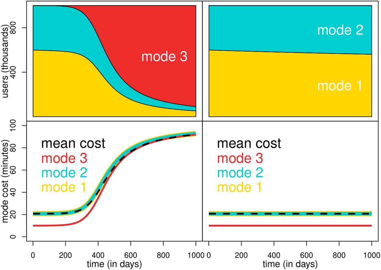
FIGURE 7. Modal share (top) and commuting time in minutes (bottom) as the dynamical system evolves in some dimensionless units, marked as “days”. The top left panel has a small (positive) initial number of users for mode 3. The right panel has zero initial users for mode 3, resembling the scenario where that mode will never exist. The baseline commuting time of mode 3 is below the observed commuting time for modes 1 and 2, so the red line has a lower cost than the initial condition. As more users are attracted by the faster mode 3, this mode becomes slower, but also, other modes experience higher induced costs. Only if all users pick mode 3, the commuting time of all modes is the same (thus becoming an equilibrium). Otherwise, the commuting time is always lower for mode 3. The average commuting time (dashed line) increases when mode 3 attracts more users. With these parameters, regardless of the initial internal conditions, the long-term distribution is that everyone chooses mode 3. However, when x₃(t) = 0 (right panel), the system converges to a separate equilibrium, where the long-term mean commuting time is significantly lower.

The scenario where most users are tempted by a “fast” commuting mode that imposes high direct and indirect costs on others (left panel of Figure 7) might create trajectories that are mostly tragic (bottom right panel of Figure 6). The imposed costs compensate whatever gain that switching individuals might have, so the mean commuting time increases after switching. Under these conditions, the city will converge to most users in mode 3, experiencing high commuting times (on average, 100 min) against the scenario where the commuting method remains unknown (right panel of Figure 7), where the average commuting times remain close to 20 min.

Novel modal shares might alter the equilibrium, although it takes time for the replicator dynamics to fully adhere them into the system. For example, a city with N = 1, 000, 000 inhabitants, with x₁(0) = 1, with x₂(0) = 400, 000 and x₃(0) = 599, 999, the equilibrium between only two modes is reached quickly and for many steps, the number of x₁ remains almost negligible (Figure 7). After a significant time, x₁ is “a hidden gem” since it has a lower commuting time (since almost nobody knows about it) and remains fast but unpopular. Eventually, x₁ becomes a popular strategy and then even a dominant modal share, reducing the size of x₂ and x₃. With any x₁(0) > 0 small, the modal share eventually attracts most people. However, if x₁(0) = 0, the equilibrium would remain on the boundary, with x₁(t) = 0 for all t ≥ 0.

3 Discussion

Our model is a simplified system (game) of users (players) that choose a commuting method (strategy) and experience some travel time (reward or cost). Detecting precisely the baseline and induced costs of a system with varying conditions, such as rain, snow, a massive event or a road accident, is an impossible task. Also, the costs that users of different transport modes impose on others are not only experienced only by an increasing commuting time, but they should include other aspects such as the use of space in a city, transport emissions, the pollution created when manufacturing cars, noise, and even the risk of suffering an accident. Also, the costs experienced due to congestion do not increase linearly with more users. Rather, each transport mode might have a different saturation point, after which users experience a steep increase in travel times [63–65]. Therefore, our model should be thought of as a simplified description of a city, its mobility and the different scenarios that might exist. A fixed baseline and linear cost functions are a simple mechanism to model the dynamics of switching between different transport modes, define trajectories and detect if a modal share is tragic, meaning that people will decrease their travel time, but this will increase the average commuting time. Other models considering urban density [35] and the distance between residence and employment have also been considered to reduce the burden of cars in cities [35, 36, 82].

Many social dilemmas might create a tragedy formed by the discrepancy between individual and collective utility, for example, regarding pollution, hoarding, and more. In our transport model, an equilibrium exists in the collective modal share, but the average commuting time is almost always higher than an efficient distribution. Therefore, a tragedy almost always exists. The tragedy goes beyond commuting times. Longer commuting times mean less productivity and less leisure time, more pollution and a collective demand for even more budget and space in cities. Thus, there is a need to understand the emergence of a tragedy and find ways to reduce its social burden.

Cities evolve depending on the ever-changing baseline time and the induced and direct costs for each commuting method. A new bike lane, an additional bus station or reducing the parking spaces in some neighbourhoods will change the conditions of the system, taking the city to a newly formed equilibrium. The city will slowly move through trajectories and, in many cases, increase the average commuting time due to individual action.

There are numerous ways in which the price of the tragedy can be contained or reduced, for instance, through cooperation, reputation [83], or creating institutions for collective action [4]. In terms of transport, many aspects promote a sustainable commute, including road pricing [37, 84] and more travel options beyond cars, such as safer cycle lanes, accessible and efficient public transport and paths which encourage people to walk [85] will reduce the tragic outcome of a car-dominated city [18]. Also, new routing strategies that aim to reduce the social cost by considering negative externalities are being studied [86, 87]. However, as long as driving is perceived as a better and faster commuting option than using the public transport, many people will eventually drive [88]. Thus, efforts to promote a sustainable mobility should focus on improving public transport and the walking and cycling experience in cities [47].

The car is a transport method with a small baseline commuting time. It might be perceived as comfortable and fast, so cars might be an attractive mode of commuting in many cities. However, it has high induced and direct costs. Cars require too much road infrastructure for moving and for parking, imposing an inefficient and costly use of space. Cars lower the available space for public transport, put cyclists at risk and reduce space for pedestrians. In some US cities, such as Atlanta, more than 90% of the daily journeys of commuters are by car, so the city has evolved, creating more space for cars and less room for anything else. We see that cars have imposed an enormous cost on cycling, public transport, or walking, making it very difficult not to depend on a vehicle for individual mobility. A new technology introduced, as seen when cars were introduced a few decades ago, or more recently with the start of shared services, might result in an actual increase in the miles travelled and the commuting times [81].

Individualistic behaviour might lead us to a tragedy where the outcomes are far from sustainable cities. Hence, reducing the discrepancy between the modal share in equilibrium and the social optimum must be central in sustainable policies for transportation.

3.1 How to Implement This Model in a Real-Case Scenario?

Changing commuting behaviour is not easy [37]. Two elements are needed to detect the tragedy of transport in a city: first, we need to understand the reasons why people drive and second, also understanding the attitudes of those who do not drive. Using origin-destination surveys that capture details about the journeys and attitudes, it is possible to uncover current and future trends for mobility in a city. Different socioeconomic groups make travel mode decisions based on various factors [89]. For example, a study showed that nearly one in five people in Mexico City would use a car if they could pay for it [88, 90]. Although the Metro System in Mexico City has nearly five million passengers per day, a considerable part of the public transport users in the city is made up of captive riders who do not have an alternative mode of travel [20]. However, it is likely that many people will shift to driving as soon as they can afford it.

All transport modes have some degree of undesirability [46] and although we have used time units to quantify this factor, understanding the main reasons for choosing a commuting method is critical for reducing the size of the tragedy. Many people might avoid public transport if it is perceived as unsafe, unreliable, uncomfortable or inaccessible [91], including pedestrian safety [92], neighbourhood amenities [93] and the urban form [94].

4 Methods

4.1 Existence of an Internal Equilibrium

Without loss of generality, considering only κ = 3 commuting options, for method i, the commuting time is higher when all users choose that mode. To see this, let x = (x, y, z). We can write the commuting time as

$C_i\left(x,y,z\right)=B_i+\alpha x+\beta y+\gamma z\text{,\hspace{0.17em}with}i=\mathrm{1,2}\text{and\hspace{0.17em}}3\text{,}(7)$

where x + y + z = N, and where α, β and γ are parameters. For x = N we get that C_i(N, 0, 0) = B_i + αN, but, if x = N − r, it means r users with a different method, so C_i(N − r, s, r − s) = B_i + α(N − r) + βs + γ(r − s), thus, the commuting time is reduced in r units of α and increases in either βs and γ(r − s), for some s ∈ [0, r]. Let δ = max(β, γ) < α be the largest induced cost. Then,

$C_i\left(N,\mathrm{0,0}\right)=B_i+\alpha N(8)$

$>B_i+\alpha \left(N-r\right)+\delta s+\delta \left(r-s\right)(9)$

$\ge B_i+\alpha \left(N-r\right)+\beta s+\gamma \left(r-s\right)=C_i\left(N-r,s,r-s\right).(10)$

Therefore, when everyone uses method i, its commuting time C_i(N, 0, 0) is higher than the commuting time of other modes.

Assuming that for all transport modes, there is some modal share for which the commuting time is lower than other transport modes, means that all transport modes are the slowest and the fastest method for different shares. Consider only two transport modes. Their commuting time surface C₁ and C₂ (a plane from the simplex X₃ to R⁺) intersects on a non-empty line, that is, a set U_1,2 for which the commuting time of both transport modes are equal. The set U_1,2 divides the simplex into two parts, one for which mode 1 has a higher commuting time (which contains the corner of S₃ where all journeys are via mode 1) and one where mode 2 has a higher commuting time (which contains the corner of S₃ where all journeys are on mode 2). Since U_1,2 divides the simplex into two parts, it intersects the edge where no one uses mode 3 into two parts, so that the corresponding corners of S₃ are slower for each transport mode. For modes 2 and 3, there is also a set U_2,3 which also divides X₃ into two parts as well that intersects the edge where nobody uses transport 1. We will show that U_1,2 and U_2,3 intersect at some point by contradiction. Suppose they do not intersect. This means that U_2,3 is fully contained either in the set where mode 1 is slower or fully contained in the set where mode 2 is slower. Suppose it is fully contained in the set where mode 2 is slower. This means that the simplex can be divided into three regions: one in which mode 2 is slower than both methods (the region which contains the corner of X₃ where all journeys are on transport 2), one in which mode 1 is faster than the other two methods (and contains the corner where all journeys are on mode 3) and one in which mode 3 is faster than the other two methods (and contains the corner where all journeys are on mode 1). This means that X₃ is divided into three parts, where mode 2 is slower than one or both of the distinct transport modes, which is a contradiction since it is assumed that mode 2 is faster than the other modes for some modal share. Similarly, if we suppose that U_2,3 is fully contained where mode 1 is slower. Then we divide the space X₃ into three regions where mode 1 is always slower than one or both of the other methods, which is also a contradiction. Therefore, there exists an internal equilibrium.

Thus, what we have shown is that, with linear costs and a fixed baseline, all modal shares are desirable when they have zero users and the worst option when everyone uses them., and also, that a unique internal equilibrium exists. Therefore, we can also ensure that all trajectories with an internal initial condition, will converge to that equilibrium.

4.2 Finding the Minimum Mean Commuting Time

Let f(r, s) = rC₁(r, s, N − r − s) + sC₂(r, s, N − r − s) + (N − r − s)C₃(r, s, N − r − s) be the total commuting time of the modal share (r, s, N − r − s) for some 0 ≤ r + s ≤ N. The function f can then be expressed as

$f\left(r,s\right)=D{r}^2+Ers+F{s}^2+Gr+Hs+I,(11)$

where

$D=M_{11}-M_{13}-M_{31}+M_{33}(12)$

$E=M_{12}-M_{13}+M_{21}-M_{23}-M_{31}-M_{32}+2M_{33}(13)$

$F=M_{22}-M_{23}-M_{32}+M_{33}(14)$

$G=B_1-B_3+N{M}_{13}+N{M}_{31}-2N{M}_{33}(15)$

$H=B_2-B_3+N{M}_{23}+N{M}_{32}-2N{M}_{33}\text{,\hspace{0.17em}and}(16)$

$I=N{B}_3+N^2{M}_{33}.(17)$

Evaluating f(N, 0) = N²M₁₁ + NB₁ and similarly, for f(0, N) = N²M₂₂ + NB₂, gives the total commuting time for N users of the first and second commuting methods. The expression f(0, 0) = N²M₃₃ + NB₃ gives the total commuting time when the third method has N users. The function f is a quadratic polynomial that has three local maximum values in the corners of its domain 0 ≤ r + s ≤ N and therefore, there exists a point (r^*, s^*) that minimises the values of f.

The gradient of f gives

$\nabla f\left(r,s\right)=\left(\frac{\partial f}{\partial r},\frac{\partial f}{\partial s}\right)=\left(2Dr+Es+G,Er+2Fs+H\right),(18)$

and by setting the values equal to (0, 0) we get that $r^{*}=\frac{2FG-EH}{E^2-4DF}\text{,\hspace{0.17em}and\hspace{0.17em}}{s}^{*}=\frac{2DH-EG}{E^2-4DF}$. Therefore, we can compute N − r^* − s^* and obtain the optimum modal share, (r^*, s^*, N − r^* − s^*).

4.3 A Stable Equilibrium

Using the same function f(r, s) as introduced before, we know that the system is in equilibrium if C₁(r, s, N − r − s) = C₂(r, s, N − r − s) = C₃(r, s, N − r − s) from which we get that r° = (WY − VZ)/(UY − VX) and s° = (WX − UZ)/(VX − UY), where the coefficients are

$U=M_{11}-M_{13}-M_{21}+M_{23}(19)$

$V=M_{12}-M_{13}-M_{22}+M_{23}(20)$

$W=B_2-B_1+N{M}_{23}-N{M}_{13}(21)$

$X=M_{11}-M_{13}-M_{31}+M_{33}(22)$

$Y=M_{12}-M_{13}-M_{32}+M_{33}\text{,\hspace{0.17em}and}(23)$

$Z=B_3-B_1+N{M}_{33}-N{M}_{13}.(24)$

From these two equations for (r°, s°, N − r° − s°) the conditions for an equilibrium point in the modal share can now be found. In general, r° ≠ r^* and s° ≠ s^* meaning that the modal share with minimum mean commuting time is not the modal share observed at equilibrium. Under certain conditions, however, it is possible that r° = r^* and s° = s^*. In terms of the induced costs, there is one case, where M₁₂ = M₁₃ = M₂₁ = M₂₃ = M₃₁ = M₃₂, in terms of the direct costs, M₁₁ = M₂₂ = M₃₃ and the baseline commuting time B₁ = B₂ = B₃. Such a scenario happens when all transport modes have the same baseline commuting time and the same induced and direct costs with respect to the other modes. Since P₁ + P₂ + P₃ = N, then the commuting time for some transport mode can be expressed as $C_i(P_i)=B_i^0+m{P}_i$, where the commuting time only depends on the number of users of the chosen method of transport, $B_i^0$ considers all induced costs and the gradient m is the difference between the direct and induced costs. In such a case, the matrix $\mathcal{M}$ in Eq. 2 is diagonal. The equilibrium from the system x° = (r°, s°, N − r° − s°) and the optimum modal share, x^* = (r^*, s^*, N − r^* − s^*) are the same. Moreover, the optimum and stable equilibrium is reached with a modal share corresponding to (N/3, N/3, N/3), meaning that all transport modes attract the same number of users. Except for this scenario, we observe that (r°, s°, N − r° − s°) ≠ (r^*, s^*, N − r^* − s^*), meaning that the stable point in the replicator dynamics is not the system optimum.

Data Availability Statement

The original contributions presented in the study are included in the article. Further inquiries can be directed to the corresponding author.

Author Contributions

RPC designed the study. RPC and HGR analysed the results. All authors wrote the manuscript.

Funding

This project received financial support from the PEAK Urban programme, funded by UKRI’s Global Challenge Research Fund, grant no. ref.: PES/P011055/1. The research was funded by the Austrian Federal Ministry for Climate Action, Environment, Energy, Mobility, Innovation and Technology under grant number 2021-0.664.668 and also from the PEAK Urban programme, funded by UKRI's Global Challenge Research Fund, grant no. ref.: PES/P011055/1.

Conflict of Interest

The authors declare that the research was conducted in the absence of any commercial or financial relationships that could be construed as a potential conflict of interest.

Publisher’s Note

All claims expressed in this article are solely those of the authors and do not necessarily represent those of their affiliated organizations, or those of the publisher, the editors and the reviewers. Any product that may be evaluated in this article, or claim that may be made by its manufacturer, is not guaranteed or endorsed by the publisher.

References

1. Lloyd WF. Two Lectures on the Checks to Population. Oxford, UK: JH Parker (1833).

Google Scholar

2. Hardin G. The Tragedy of the Commons. Science (1968) 162(3859):1243–8. doi:10.1126/science.162.3859.1243

PubMed Abstract | CrossRef Full Text | Google Scholar

3. Rankin DJ, Bargum K, Kokko H. The Tragedy of the Commons in Evolutionary Biology. Trends Ecol Evol (2007) 22:643–51. doi:10.1016/j.tree.2007.07.009

PubMed Abstract | CrossRef Full Text | Google Scholar

4. Ostrom E. Governing the Commons: The Evolution of Institutions for Collective Action. Cambridge, UK: Cambridge University Press (1990).

Google Scholar

5. Couclelis H. From Sustainable Transportation to Sustainable Accessibility: Can We Avoid a New Tragedy of the Commons? In: Information, Place, and Cyberspace. Berlin, Germany: Springer (2000). p. 341–56. doi:10.1007/978-3-662-04027-0_20

CrossRef Full Text | Google Scholar

6. Mogridge MJ. The Self-Defeating Nature of Urban Road Capacity Policy. Transport Policy (1997) 4:5–23. doi:10.1016/s0967-070x(96)00030-3

CrossRef Full Text | Google Scholar

7. Duranton G, Turner MA. The Fundamental Law of Road Congestion: Evidence from US Cities. Am Econ Rev (2011) 101:2616–52. doi:10.1257/aer.101.6.2616

CrossRef Full Text | Google Scholar

8. Çolak S, Lima A, González MC. Understanding Congested Travel in Urban Areas. Nat Commun (2016) 7:10793–8. doi:10.1038/ncomms10793

PubMed Abstract | CrossRef Full Text | Google Scholar

9. Prieto Curiel R, González Ramírez H, Quiñones Domínguez M, Orjuela Mendoza JP. A Paradox of Traffic and Extra Cars in a City as a Collective Behaviour. R Soc Open Sci (2021) 8:201808. doi:10.1098/rsos.201808

PubMed Abstract | CrossRef Full Text | Google Scholar

10. De Vos J, Mokhtarian PL, Schwanen T, Van Acker V, Witlox F. Travel Mode Choice and Travel Satisfaction: Bridging the gap between Decision Utility and Experienced Utility. Transportation (2016) 43:771–96. doi:10.1007/s11116-015-9619-9

CrossRef Full Text | Google Scholar

11. Liao Y, Gil J, Pereira RHM, Yeh S, Verendel V. Disparities in Travel Times between Car and Transit: Spatiotemporal Patterns in Cities. Sci Rep (2020) 10:4056–12. doi:10.1038/s41598-020-61077-0

PubMed Abstract | CrossRef Full Text | Google Scholar

12. Beirão G, Cabral JS. Understanding Attitudes towards Public Transport and Private Car: A Qualitative Study. Transport Policy (2007) 14:478–89. doi:10.1016/j.tranpol.2007.04.009

CrossRef Full Text | Google Scholar

13. van Exel NJA, Rietveld P. Perceptions of Public Transport Travel Time and Their Effect on Choice-Sets Among Car Drivers. J Transport Land Use (2010) 2:75–86. doi:10.5198/jtlu.v2i3.15

CrossRef Full Text | Google Scholar

14. Farber S, Fu L. Dynamic Public Transit Accessibility Using Travel Time Cubes: Comparing the Effects of Infrastructure (Dis) Investments over Time. In: Computers, Environment and Urban Systems. London, UK: Elsevier, 62 (2017). p. 30–40.

CrossRef Full Text | Google Scholar

15. Eriksson L, Friman M, Gärling T. Stated Reasons for Reducing Work-Commute by Car. In: Transportation Research Part F: Traffic Psychology and Behaviour. London, UK: Elsevier, 11 (2008). p. 427–33. doi:10.1016/j.trf.2008.04.001

CrossRef Full Text | Google Scholar

16. Redman L, Friman M, Gärling T, Hartig T. Quality Attributes of Public Transport that Attract Car Users: A Research Review. Transport Policy (2013) 25:119–27. doi:10.1016/j.tranpol.2012.11.005

CrossRef Full Text | Google Scholar

17. Schäfer AW. Long-term Trends in Domestic US Passenger Travel: the Past 110 Years and the Next 90. Transportation (2017) 44:293–310. doi:10.1007/s11116-015-9638-6

CrossRef Full Text | Google Scholar

18. Zhou J. Sustainable Commute in a Car-Dominant City: Factors Affecting Alternative Mode Choices Among University Students. In: Transportation Research Part A: Policy and Practice. London, UK: Elsevier, 46 (2012). p. 1013–29. doi:10.1016/j.tra.2012.04.001

CrossRef Full Text | Google Scholar

19. Mohring H. Optimization and Scale Economies in Urban Bus Transportation. Am Econ Rev (1972) 62:591–604.

Google Scholar

20. Bar-Yosef A, Martens K, Benenson I. A Model of the Vicious Cycle of a Bus Line. In: Transportation Research Part B: Methodological. London, UK: Elsevier, 54 (2013). p. 37–50. doi:10.1016/j.trb.2013.03.010

CrossRef Full Text | Google Scholar

21. Levinson DM, Krizek KJ. Planning for Place and Plexus: Metropolitan Land Use and Transport. New York, USA: Routledge (2007).

Google Scholar

22. Reinhold T. More Passengers and Reduced Costs—The Optimization of the Berlin Public Transport Network. J Public Transportation (2008) 11:4. doi:10.5038/2375-0901.11.3.4

CrossRef Full Text | Google Scholar

23. Katz D, Rahman MM. Levels of Overcrowding in Bus System of Dhaka, Bangladesh. Transportation Res Rec (2010) 2143:85–91. doi:10.3141/2143-11

CrossRef Full Text | Google Scholar

24. Varghese V, Adhvaryu B. Measuring Overcrowding in Ahmedabad Buses: Costs and Policy Implications. Transportation Res Proced (2016) 17:145–54. doi:10.1016/j.trpro.2016.11.070

CrossRef Full Text | Google Scholar

25. Samson BPV, Aldanese IV CR, Chan DMC, San Pascual JJS, Sido MVAP. Crowd Dynamics and Control in High-Volume Metro Rail Stations. Proced Comput Sci (2017) 108:195–204. doi:10.1016/j.procs.2017.05.097

CrossRef Full Text | Google Scholar

26. Banister D. Cities, Mobility and Climate Change. J Transport Geogr (2011) 19:1538–46. doi:10.1016/j.jtrangeo.2011.03.009

CrossRef Full Text | Google Scholar

27. Smeed RJ. The Traffic Problem in Towns. Town Plann Rev (1964) 35:133–58. doi:10.3828/tpr.35.2.n482755235577655

CrossRef Full Text | Google Scholar

28. Maerivoet S, De Moor B. Transportation Planning and Traffic Flow Models. Ithaca, USA: ArXiv (2005). arXiv preprint physics/0507127.

Google Scholar

29. Pigou AC. The Economics of Welfare. London: Palgrave Macmillan (1920).

Google Scholar

30. Brand C, Dons E, Anaya-Boig E, Avila-Palencia I, Clark A, de Nazelle A, et al. The Climate Change Mitigation Effects of Daily Active Travel in Cities. Transportation Res D: Transport Environ (2021) 93:102764. doi:10.1016/j.trd.2021.102764

CrossRef Full Text | Google Scholar

31. Saunders LE, Green JM, Petticrew MP, Steinbach R, Roberts H. What Are the Health Benefits of Active Travel? A Systematic Review of Trials and Cohort Studies. PLoS One (2013) 8:e69912. doi:10.1371/journal.pone.0069912

PubMed Abstract | CrossRef Full Text | Google Scholar

32. Keall MD, Shaw C, Chapman R, Howden-Chapman P. Reductions in Carbon Dioxide Emissions from an Intervention to Promote Cycling and Walking: A Case Study from New Zealand. In: Transportation Research Part D: Transport and Environment. London, UK: Elsevier, 65 (2018). p. 687–96. doi:10.1016/j.trd.2018.10.004

CrossRef Full Text | Google Scholar

33. Petrunoff N, Rissel C, Wen LM, Martin J. Carrots and Sticks vs Carrots: Comparing Approaches to Workplace Travel Plans Using Disincentives for Driving and Incentives for Active Travel. J Transport Health (2015) 2:563–7. doi:10.1016/j.jth.2015.06.007

CrossRef Full Text | Google Scholar

34. Schafer A, Victor DG. The Future Mobility of the World Population. Transportation Res A: Pol Pract (2000) 34:171–205. doi:10.1016/s0965-8564(98)00071-8

CrossRef Full Text | Google Scholar

35. Newman PG, Kenworthy JR. Cities and Automobile Dependence: An International Sourcebook. VT United States: Gower Publishing, Brookfield (1989).

Google Scholar

36. Verbavatz V, Barthelemy M. Critical Factors for Mitigating Car Traffic in Cities. PLoS One (2019) 14:e0219559. doi:10.1371/journal.pone.0219559

PubMed Abstract | CrossRef Full Text | Google Scholar

37. Kristal AS, Whillans AV. What We Can Learn from Five Naturalistic Field Experiments that Failed to Shift Commuter Behaviour. Nat Hum Behav (2020) 4:169–76. doi:10.1038/s41562-019-0795-z

PubMed Abstract | CrossRef Full Text | Google Scholar

38. Neumann JV, Morgenstern O. Theory of Games and Economic Behavior. Princeton, USA: Princeton University Press (1944).

Google Scholar

39. Marschak J. Binary Choice Constraints on Random Utility Indicators. New Haven, USA: Cowles Foundation for Research in Economics, Yale University (1959). Cowles Foundation Discussion Papers 74.

Google Scholar

40. McFadden D. Conditional Logit Analysis of Qualitative Choice Behavior. In: P Zarembka, editor. Frontiers of Econometrics. (Berkeley, USA: Berkeley University Press) (1972).

Google Scholar

41. McFadden D, Train K. Mixed MNL Models for Discrete Response. J Appl Econ (2000) 15:447–70. doi:10.1002/1099-1255(200009/10)15:5<447::aid-jae570>3.0.co;2-1

CrossRef Full Text | Google Scholar

42. Al-Widyan F, Kirchner N, Zeibots M. An Empirically Verified Passenger Route Selection Model Based on the Principle of Least Effort for Monitoring and Predicting Passenger Walking Paths through Congested Rail Station Environments. In: Australasian Transport Research Forum 2015 Proceedings. Australia: Australasian Transport Research Forum Incorporated (2015). p. 1–12.

Google Scholar

43. Wardrop JG. Road Paper. Some Theoretical Aspects of Road Traffic Research. Proc Inst Civil Eng (1952) 1:325–62. doi:10.1680/ipeds.1952.11259

CrossRef Full Text | Google Scholar

44. Daganzo CF, Sheffi Y. On Stochastic Models of Traffic Assignment. Transportation Sci (1977) 11:253–74. doi:10.1287/trsc.11.3.253

CrossRef Full Text | Google Scholar

45. Mahmassani HS, Chang G-L. On Boundedly Rational User Equilibrium in Transportation Systems. Transportation Sci (1987) 21:89–99. doi:10.1287/trsc.21.2.89

CrossRef Full Text | Google Scholar

46. Downs A. The Law of Peak-Hour Expressway Congestion. Traffic Q (1962) 16.

Google Scholar

47. Thomson JM. Great Cities and Their Traffic. Middlesex, UK: Penguin Books (1978).

Google Scholar

48. Selten R, Chmura T, Pitz T, Kube S, Schreckenberg M. Commuters Route Choice Behaviour. Games Econ Behav (2007) 58:394–406. doi:10.1016/j.geb.2006.03.012

CrossRef Full Text | Google Scholar

49. Rapoport A, Kugler T, Dugar S, Gisches EJ. Braess Paradox in the Laboratory: Experimental Study of Route Choice in Traffic Networks with Asymmetric Costs. New York, USA: Springer (2008).

Google Scholar

50. Sheffi Y. Urban Transportation Networks. Englewood Cliffs, USA: Prentice-Hall (1985). p. 415. doi:10.1016/0191-2607(86)90023-3

CrossRef Full Text | Google Scholar

51. Correa JR, Schulz AS, Stier-Moses NE. On the Inefficiency of Equilibria in Congestion Games. In: International Conference on Integer Programming and Combinatorial Optimization. Berlin, Germany: Springer (2005). p. 167–81. doi:10.1007/11496915_13

CrossRef Full Text | Google Scholar

52. Roughgarden T. Selfish Routing and the price of Anarchy, 174. USA, Cambridge): MIT Press (2005).

Google Scholar

53. Koutsoupias E, Papadimitriou C. Worst-case Equilibria. In: Annual Symposium on Theoretical Aspects of Computer Science. Berlin, Germany: Springer (1999). p. 404–13. doi:10.1007/3-540-49116-3_38

CrossRef Full Text | Google Scholar

54. Roughgarden T, Tardos É. How Bad Is Selfish Routing? J Acm (2002) 49:236–59. doi:10.1145/506147.506153

CrossRef Full Text | Google Scholar

55. Youn H, Gastner MT, Jeong H. Price of Anarchy in Transportation Networks: Efficiency and Optimality Control. Phys Rev Lett (2008) 101. doi:10.1103/physrevlett.101.128701

PubMed Abstract | CrossRef Full Text | Google Scholar

56. Roughgarden T. Compact Cities Sustainable Urban Forms for Developing Countries. Cambridge, MA: MIT Press (2006).

Google Scholar

57. Cohen JE. Cooperation and Self-Interest: Pareto-Inefficiency of Nash Equilibria in Finite Random Games. Proc Natl Acad Sci U.S.A (1998) 95:9724–31. doi:10.1073/pnas.95.17.9724

PubMed Abstract | CrossRef Full Text | Google Scholar

58. Krueger AB, Kahneman D, Schkade D, Schwarz N, Stone AA. National Time Accounting: The Currency of Life. In: Measuring the Subjective Well-Being of Nations: National Accounts of Time Use and Well-Being. Chicago, USA: University of Chicago Press (2009). p. 9–86.

Google Scholar

59. Kölbl R, Helbing D. Energy Laws in Human Travel Behaviour. New J Phys (2003) 5:48. doi:10.1088/1367-2630/5/1/348

CrossRef Full Text | Google Scholar

60. Ceder A. Public Transit Planning and Operation: Modeling, Practice and Behavior. Florida, USA: CRC Press (2016).

Google Scholar

61. Branston D. Link Capacity Functions: A Review. Transportation Res (1976) 10:223–36. doi:10.1016/0041-1647(76)90055-1

CrossRef Full Text | Google Scholar

62. Rose G, Taylor MAP, Tisato P. Estimating Travel Time Functions for Urban Roads: Options and Issues. Transportation Plann Techn (1989) 14:63–82. doi:10.1080/03081068908717414

CrossRef Full Text | Google Scholar

63. Davis GA, Xiong H. Access to Destinations: Travel Time Estimation on Arterials (2007). Report 3, Access to Destination Studies. Minnesota, USA: Minnesota Department of Transportation.

Google Scholar

64. Guessous Y, Aron M, Bhouri N, Cohen S. Estimating Travel Time Distribution under Different Traffic Conditions. Transportation Res Proced (2014) 3:339–48. doi:10.1016/j.trpro.2014.10.014

CrossRef Full Text | Google Scholar

65. Maerivoet S, De Moor B. Traffic Flow Theory (2005). arXiv preprint physics/0507126. Ithaca, USA: ArXiv.

Google Scholar

66. Louf R, Barthelemy M. Modeling the Polycentric Transition of Cities. Phys Rev Lett (2013) 111:198702. doi:10.1103/physrevlett.111.198702

PubMed Abstract | CrossRef Full Text | Google Scholar

67. Ewing R, Cervero R. Travel and the Built Environment. J Am Plann Assoc (2010) 76:265–94. doi:10.1080/01944361003766766

CrossRef Full Text | Google Scholar

68. Taylor PD, Jonker LB. Evolutionary Stable Strategies and Game Dynamics. Math Biosciences (1978) 40:145–56. doi:10.1016/0025-5564(78)90077-9

CrossRef Full Text | Google Scholar

69. Hofbauer J, Sigmund K. Evolutionary Game Dynamics. Bull Amer Math Soc (2003) 40:479–519. doi:10.1090/s0273-0979-03-00988-1

CrossRef Full Text | Google Scholar

70. Ohtsuki H, Nowak MA. The Replicator Equation on Graphs. J Theor Biol (2006) 243:86–97. doi:10.1016/j.jtbi.2006.06.004

PubMed Abstract | CrossRef Full Text | Google Scholar

71. Hofbauer J, Schuster P, Sigmund K. A Note on Evolutionary Stable Strategies and Game Dynamics. J Theor Biol (1979) 81:609–12. doi:10.1016/0022-5193(79)90058-4

PubMed Abstract | CrossRef Full Text | Google Scholar

72. Maynard Smith J. Evolution and the Theory of Games. Cambridge, UK: Cambridge University Press (1982).

Google Scholar

73. Nowak MA, Sigmund K. Evolutionary Dynamics of Biological Games. Science (2004) 303:793–9. doi:10.1126/science.1093411

PubMed Abstract | CrossRef Full Text | Google Scholar

74. Nash JF. Equilibrium Points in N -person Games. Proc Natl Acad Sci U.S.A (1950) 36:48–9. doi:10.1073/pnas.36.1.48

PubMed Abstract | CrossRef Full Text | Google Scholar

75. May RM. Simple Mathematical Models with Very Complicated Dynamics. In: The Theory of Chaotic Attractors. New York, USA: Springer (2004). p. 85–93. doi:10.1007/978-0-387-21830-4_7

CrossRef Full Text | Google Scholar

76. Gardiner SM. The Real Tragedy of the Commons. Philos Public Aff (2001) 30:387–416. doi:10.1111/j.1088-4963.2001.00387.x

PubMed Abstract | CrossRef Full Text | Google Scholar

77. Erhardt GD, Roy S, Cooper D, Sana B, Chen M, Castiglione J. Do transportation Network Companies Decrease or Increase Congestion? Sci Adv (2019) 5:eaau2670. doi:10.1126/sciadv.aau2670

PubMed Abstract | CrossRef Full Text | Google Scholar

78. Lavieri PS, Bhat CR. Investigating Objective and Subjective Factors Influencing the Adoption, Frequency, and Characteristics of Ride-Hailing Trips. Transportation Res C: Emerging Tech (2019) 105:100–25. doi:10.1016/j.trc.2019.05.037

CrossRef Full Text | Google Scholar

79. Rayle L, Dai D, Chan N, Cervero R, Shaheen S. Just a Better Taxi? a Survey-Based Comparison of Taxis, Transit, and Ridesourcing Services in San Francisco. Transport Policy (2016) 45:168–78. doi:10.1016/j.tranpol.2015.10.004

CrossRef Full Text | Google Scholar

80. Clewlow RR, Mishra GS. Disruptive Transportation: The Adoption, Utilization, and Impacts of Ride-Hailing in the United States. UC Davis: Institute of Transportation Studies (2017). Tech. rep.

Google Scholar

81. Schaller B. Can Sharing a Ride Make for Less Traffic? Evidence from Uber and Lyft and Implications for Cities. Transport Policy (2021) 102:1–10. doi:10.1016/j.tranpol.2020.12.015

CrossRef Full Text | Google Scholar

82. Fujita M, Ogawa H. Multiple Equilibria and Structural Transition of Non-monocentric Urban Configurations. Reg Sci Urban Econ (1982) 12:161–96. doi:10.1016/0166-0462(82)90031-x

CrossRef Full Text | Google Scholar

83. Milinski M, Semmann D, Krambeck H-J. Reputation Helps Solve the 'Tragedy of the Commons'. Nature (2002) 415:424–6. doi:10.1038/415424a

PubMed Abstract | CrossRef Full Text | Google Scholar

84. Dieplinger M, Fürst E. The Acceptability of Road Pricing: Evidence from Two Studies in Vienna and Four Other European Cities. Transport Policy (2014) 36:10–8. doi:10.1016/j.tranpol.2014.06.012

CrossRef Full Text | Google Scholar

85. Quastel N, Moos M, Lynch N. Sustainability-as-density and the Return of the Social: The Case of Vancouver, British Columbia. Urban Geogr (2012) 33:1055–84. doi:10.2747/0272-3638.33.7.1055

CrossRef Full Text | Google Scholar

86. van Essen M, Thomas T, van Berkum E, Chorus C. Travelers' Compliance with Social Routing Advice: Evidence from SP and RP Experiments. Transportation (2020) 47:1047–70. doi:10.1007/s11116-018-9934-z

CrossRef Full Text | Google Scholar

87. Mariotte G, Leclercq L, Gonzalez Ramirez H, Krug J, Bécarie C. Assessing Traveler Compliance with the Social Optimum: A Stated Preference Study. Trav Behav Soc (2021) 23:177–91. doi:10.1016/j.tbs.2020.12.005

CrossRef Full Text | Google Scholar

88. Suárez Lastra M, Galindo Pérez C, Reyes García V. Cómo nos movemos en la Ciudad de México. Mexico City, Mexico: Instituo de Investigaciones Jurídicas, UNAM (2019).

Google Scholar

89. Boarnet MG, Crane R. Travel by Design: The Influence of Urban Form on Travel. Oxford, UK: Oxford University Press on Demand (2001).

Google Scholar

90. Suárez Lastra M, Delgado Campos GJ. Entre mi casa y mi destino: movilidad y transporte en México: Encuesta Nacional de Movilidad y Transporte. Mexico City, Mexico: Universidad Nacional Autónoma de México, Instituto de Investigaciones Jurídicas (2015).

Google Scholar

91. Gascon M, Marquet O, Gràcia-Lavedan E, Ambròs A, Götschi T, Nazelle Ad., et al. What Explains Public Transport Use? Evidence from Seven European Cities. Transport Policy (2020) 99:362–74. doi:10.1016/j.tranpol.2020.08.009

CrossRef Full Text | Google Scholar

92. Koschinsky J, Talen E, Alfonzo M, Lee S. How Walkable Is Walker's paradise? In: Environment and Planning B: Urban Analytics and City Science. Los Angeles, USA: SAGE Journals, 44 (2017). p. 343–63. doi:10.1177/0265813515625641

CrossRef Full Text | Google Scholar

93. Elldér E. What Kind of Compact Development Makes People Drive Less? the “Ds of the Built Environment” versus Neighborhood Amenities. J Plann Educ Res (2020) 40:432–46. doi:10.1177/0739456x18774120

CrossRef Full Text | Google Scholar

94. Stevens MR. Does Compact Development Make People Drive Less? J Am Plann Assoc (2017) 83:7–18. doi:10.1080/01944363.2016.1240044

CrossRef Full Text | Google Scholar