Observations of ion upflow and 630.0 nm emission during pulsating aurora

1 Introduction

In this study, we present observations from All Sky Imagers (ASI) located at Poker Flat, AK alongside data from the Poker Flat Incoherent Scatter Radar (PFISR) from 5 February 2017 to demonstrate that pulsating aurora drive ionospheric pressure gradients, which can lead to ion upflow. The data show an association between the precipitating electrons associated with Type II ion upflow (∼ hundreds of eV) and pulsating aurora (∼ tens to hundreds of keV), and are similar to those reported in Liang et al. [1]. Furthermore, auroral red-line emission was also observed during this event. This is a new result, which suggests that ion upflow (and possibly ion outflow) can occur in different contexts than previously thought.

1.1 Pulsating aurora

Pulsating aurora is a commonly observed phenomenon Jones et al. ([2] reported 74 pulsating aurora events out of 119 days of optical data, and Partamies et al. [3] reported agreement to such an occurrence rate). This phenomenon is associated with the breakup and recovery stages of geomagnetic substorms, hence is typically observed shortly after magnetic midnight [4–6].

Pulsating aurora appears as spatially distinct regions (e.g. “patches”) of periodically varying brightness. Although these “pulsation” periods typically range from 2 to 20 s [7], the period of pulsation can vary in time (within the same event), or vary in space (across the same structure), with individual patches often pulsating out of phase with each other [8]. A typical pulsating auroral event lasts for ∼ 1.5 h [3, 9] from beginning to end, though longer events have also been reported (e.g. 7 h [3] and 15 h [2]).

Pulsating aurora often appears, cast against a steady-state, non-varying background of diffuse aurora (associated with 2–3 keV plasmasheet electrons), which represents a significant flux of energy into the ionosphere [10]. However, Brown et al. [11] demonstrated that pulsating aurora occurs at lower altitudes (82–105 km) than diffuse aurora (118–375 km), by using a triangulation method (see also Royrvik and Davis [7]). This difference in occurrence altitude is attributed to there being two separate populations of precipitating electrons driving the two different auroral phenomenon, with the higher energy population (resulting from interactions with chorus waves near the magnetic equator that scatter electrons into the loss cone [12]) driving the pulsating aurora. In this way, pulsating aurora serves as an ionospheric signature of high energy (∼ tens to hundreds of keV) electron precipitation [3, 11, 13].

Observations of pulsating aurora are most commonly reported in the 557.7 nm (green-line) and 427.8 nm (blue-line), wavelengths, which are sensitive to high energy electron precipitation. Less commonly observed is 630.0 nm (red-line) emission (produced during the transition of atomic oxygen from the first excited state to the ground state [14, 15]), which is driven by soft electron precipitation (∼ hundreds of eV) [16–18]. Depending on the modulation of the driving soft electron precipitation, the resulting red-line aurora may be observed to be pulsating or steady-state [17].

The difference between the frequency with which green-line and blue-line vs red-line auroral emissions are observed is likely due to the fact that the high energy electron precipitation that drives the pulsation deposits its energy at lower altitudes (82–105 km) where the particle density is greater. It is worth noting that red-line aurorae have been observed between 150 and 400 km, but not below 150 km since atmospheric quenching ultimately suppresses red-line emission below this threshold [16, 19].

In contrast, black aurora is the distinct lack of auroral emission, sometimes appearing as narrow regions embedded within or adjacent to pulsating auroral patches [7]. Further, black aurora has been observed between pulsating patches with different periods of pulsation, with the black aurora forming a “boundary” that appears to separate the patches [20]. Although the mechanisms that produce black aurora are yet unknown, several theories have been put forth to explain the phenomenon. It has been suggested that black aurora denote localized suppression of pitch angle scattering [21], or the relaxation of enhanced plasma pressure near the inner plasma sheet boundary [22]. It has also been suggested that black aurora indicate regions of ionospheric return currents within auroral forms [23]. The internal structure of black aurora and its relation to pulsating auroral morphology are also yet unknown.

Ultimately, pulsating aurora is a commonly occurring phenomenon that can operate for several hours at a time [24]. Despite this, few studies have investigated the ability of pulsating aurora to drive density scale-height increases in the ionosphere-thermosphere system.

1.2 Ion outflow

Before continuing, we feel that it is necessary to discuss the phenomenon of ion outflow, which is crucial to understanding this event. Ion outflow is the two-step process through which ions in the F-region ionosphere (150–800 km) gain energies sufficient to escape Earth’s gravitational field. Observations of ion upflow have typically been made in the dayside cusp [25–28], and less often in the nightside auroral zone. Fernandes et al. [29] have reported observations of upflow velocities of several hundred m/s on the nightside at F region altitudes from the MICA sounding rocket measurements. The observed ion upflow was attributed to ambipolar electric fields, though they did not rule out the frictional heating effect. Further, Ren et al. [30] conducted a statistical survey of PFISR ion upflow observations using data from 2011 to 2013, and found that ion upflow is about twice as likely to occur at the location of PFISR between 23:00 to 03:00 MLT than at the minimum occurrence rate in the noon sector.

In the first stage of this process, called upflow, ions are lifted along magnetic field lines from ∼ 100–250 km to 500 and 600 km or higher on the dayside and ∼ 400 km or higher on the nightside [30]. In the second stage in this process, called outflow, interactions with broadband extremely low frequency (BBELF) and/or very low frequency (VLF) waves at these altitudes are required to further energize upflowing particles to achieve escaping velocity. In the absence of this additional energization, upflowing particles may return to lower altitudes, resulting in downflow.

There are two known drivers of the upflow process: Type I (Joule Heating) and Type II (soft electron precipitation) [28, 31, 32]. Type I ion outflow results from ionospheric convection, which delivers heat to background ions, causing them to expand upward adiabatically. Type II ion outflow results from precipitating electrons (∼ 10–100 eV) colliding with and heating background electrons. This expanding electron gas produces a density gradient, which creates a separation of charge, resulting in an ambipolar (e.g. parallel) electric field that then accelerates ions to higher altitudes [33]. Interestingly, a hybrid of Type I and Type II ion upflow may occur in regions of discrete auroral dynamics [34, 35].

Ultimately, ion outflow facilitates the transfer of ionospheric particles into the magnetosphere, which “mass loads” the magnetosphere [31]. The process of mass loading affects plasma dynamics throughout the magnetosphere, increasing the collision rates among constituent particles [36, 37], increasing the response time of magnetic field lines, decreasing the magnetic reconnection energy transfer rate [38], and contributing to the ring current during storm times [39]. Additionally, mass loading modifies the spectral content of field line resonances [40–44], and modifies the spectral content of electromagnetic ion cyclotron waves [45–47].

2 Instrumentation

ASI, filtered for 557.7 and 630.0 nm, were run throughout the night (of 5 February 2017), while the PFISR experiment “TopsideUpflow2” was run from 12:00 to 16:00 UT. The TopsideUpflow2 observing mode consists of seven beams as shown in Figure 1, configured to provide very good statistics in the F-region and topside ionosphere.

FIGURE 1

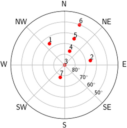
FIGURE 1. The orientation of PFISR’s 7-beam TopsideUpflow2 observing mode (in geographic coordinates). Note that Poker Flat has a magnetic declination of 16°. Beams 1 and 2 are pointed northwest and northeast respectively to allow for estimation of vector velocities. Beams 3 through 7 fan out in a plane of constant magnetic longitude. Beam 7 is oriented along the local magnetic field line (towards magnetic zenith).

In this configuration, pulses are sent out along Beams 3 through 7 three times as often as pulses in Beams 1 and 2 to optimize the statistical aspect of the data. Additionally, TopsideUpflow2 uses three frequency channels, with data from all three averaged together to improve statistics. Each outgoing pulse transmits a pair of 330 μs (corresponding to 49.5 km) pulses on two out of the three channels while the third channel collects noise samples. The pulses are 7 ms apart, yielding an effective duty cycle of 9.4%. This mode gives 50.42 independent estimates of the autocorrelation function (ACF) per second for the beams in the fan. The lag profile arrays are gated into ACFs at 24.75 km range gates, the ACFs are averaged over 5 min of data, and nonlinear least-squares fitting is used to fit the ACFs for electron number density (N_e), electron temperature (T_e), and line-of-sight velocity (v_i). It is worth noting that this observing mode was optimized for making measurements of Type II ion upflow, and hence, did not make measurements of ion temperature (T_i).

The 557.7 nm ASI data was provided by NASA Goddard Space Flight Center (GSFC) using an imager that was part of the Multi-Spectral Observatory of Sensitive EMCCD (MOOSE), installed at Poker Flat. These Andor iXon DU-888 EMCCD (Electron Multiplying Charge Coupled Device) imagers use a 1024 × 1024-pixel chip, with internal binning capabilities that allow for tradeoffs between temporal and spatial resolution. For the observations presented here, MOOSE’s imager was operating with an all-sky (180° field of view (FOV)) lens and a 557.7 nm narrowband filter (e.g. 2 nm full-width half maximum (FWHM)) bandpass. The CCD was cooled to −70 °C to reduce thermal noise and was set to 2 × 2 binning, resulting in a 512 × 512 image at 3.3 frames per second (300 ms exposure time).

The 630.0 nm data comes from a digital, EMCCD-based ASI at Poker Flat, filtered for oxygen red-line (630.0 nm), green-line (557.7 nm), and blue-line (427.8 nm) emissions. The three filters are cycled on a 12.5 s cadence. Filter bandpasses are approximately 2 nm [48].

3 Observations

The seven PFISR beams used in this study are oriented as follows. Beams 1 and 2 are pointed northwest and northeast respectively to allow for the estimation of vector velocity components. Beams 3 (vertical direction) through 7 form a “fan” within a plane of constant magnetic longitude. Beam 7 is oriented along the local magnetic field line (i.e. pointed towards magnetic zenith), making it the primary beam for observing ion upflow velocities. Beams 3, 4, 5, and 6 are intended to provide additional coverage of the ionosphere and nominally provide upflow information to support beam 7. However, as Beams 3, 4, 5, and 6 are oblique to the local magnetic field, they alone cannot determine whether or not upflow has occurred.

Figure 2 displays line-of-sight velocity data for each PFISR beam, while Figure 3 displays electron number density measurements from Beam 7. In both figures, warm colors indicate positive velocities (away from the radar) and density enhancements, while cool colors indicate negative velocities (towards the radar) and density diminutions. Above roughly 400 km the ion line-of-sight velocity data (see Figure 2) appear “speckled.” This effect results from the lower densities present in higher altitude regions. It is worth noting that, while statistics for an individual measurement can still be valid, it is prudent to interpret these plots with the understanding that several adjacent spatio-temporal bins should be demonstrating the same behavior before a valid conclusion can be drawn.

FIGURE 2

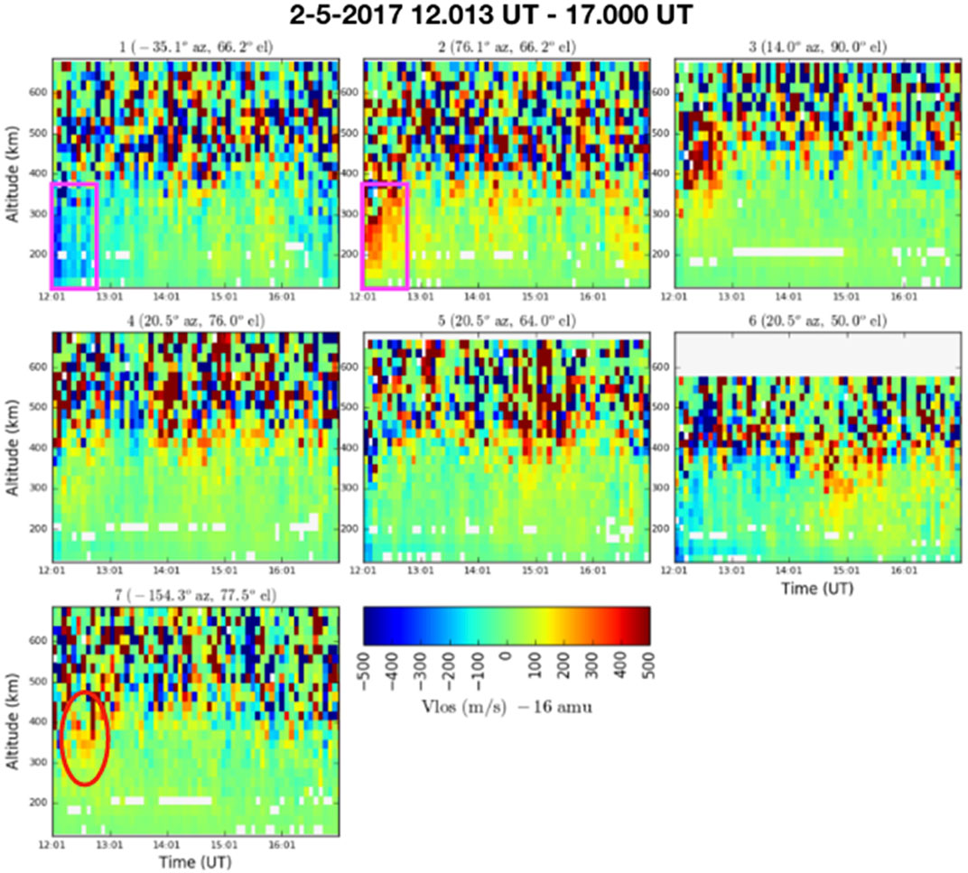
FIGURE 2. Line-of-sight velocity data for each of the seven PFISR beams. Positive values denote ion motion away from the beam, while negative values denote ion motion toward the beam. A single column within the plot represents a 5 min integration period. The vertical axis displays the height resolution of the radar pulse. The red circle indicates the ion upflow signature observed in Beam 7, while the magenta boxes highlight the convection signature present in Beams 1 and 2.

FIGURE 3

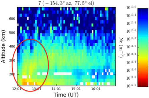
FIGURE 3. Electron number density recorded by PFISR. The red circle highlights a “plume” of ionization which is seen rising from lower altitudes close to the start of the pulsating aurora.

From 12:00 to 12:30 UT, Beams 1 and 2 recorded ion velocities corresponding to an eastward flow between ∼ 100–400 km altitude (shown in the first two panels of Figure 2, which correspond to Beams 1 and 2 respectively). The magenta boxes in Figure 2 highlight the negative velocity (towards the radar) observed by Beam 1, and the positive velocity (away from the radar) observed by Beam 2 until about 12:30 UT. This observation is not too surprising, as such flows are expected post-midnight after PFISR rotates past the Harang discontinuity [49].

The red circle in Figure 2 highlights the ion upflow signature from Beam 7 (Up-B direction), present from 12:00 to 13:00 UT, starting from 300 km, becoming stronger and increasing in altitude towards 400 km by the end of the interval. While a few temporally and spatially constrained bins show velocity enhancements in the ion data from 12:00 to 12:30 UT, the upflow signature becomes more apparent from 12:30 UT onward. Additionally, v_i enhancements are present in Beams 3 (near the same UT) and later in the evening in Beams 4, 5 and 6. However, as Beams 4, 5 and 6 are not oriented directly along the field line, it is not possible to accurately determine whether these are also signatures of upflow.

Diffuse aurora was observed earlier in the evening, followed by the pulsating aurora at ∼ 12:20 UT. Around this time, PFISR began to detect enhancements in N_e, shown in Figure 3. These enhancements appear as a “plume” of ionization (denoted by the red circle) which rose out of the E-region (90–150 km) of the ionosphere. This feature is consistent with the expanding electron gas (that in turn produces the ambipolar electric field associated with) Type II ion upflow. Alternatively, this feature may result from high energy electrons associated with pulsating aurora causing secondary ionization (see Section 5).

Examples of the associated 630.0 and 557.7 nm auroral emissions are shown in Figure 4. Within each frame, north is up, east is right, and the magnetic zenith corresponds to the region denoted by the white, dotted box (see the first frame of the second row for reference). The location of the magnetic zenith is the same in all of the frames. Pulsating aurora becomes visible predominantly in the green-line at ∼ 12:20 UT, about 10–15 min before ion upflow is observed (∼ 12:30 UT onward). Figure 4 shows the progression of the aurora beginning with the earliest onset of pulsating aurora, followed by the establishment, brightening, the breaking apart of, fading, and disappearance of the red-line structure.

FIGURE 4

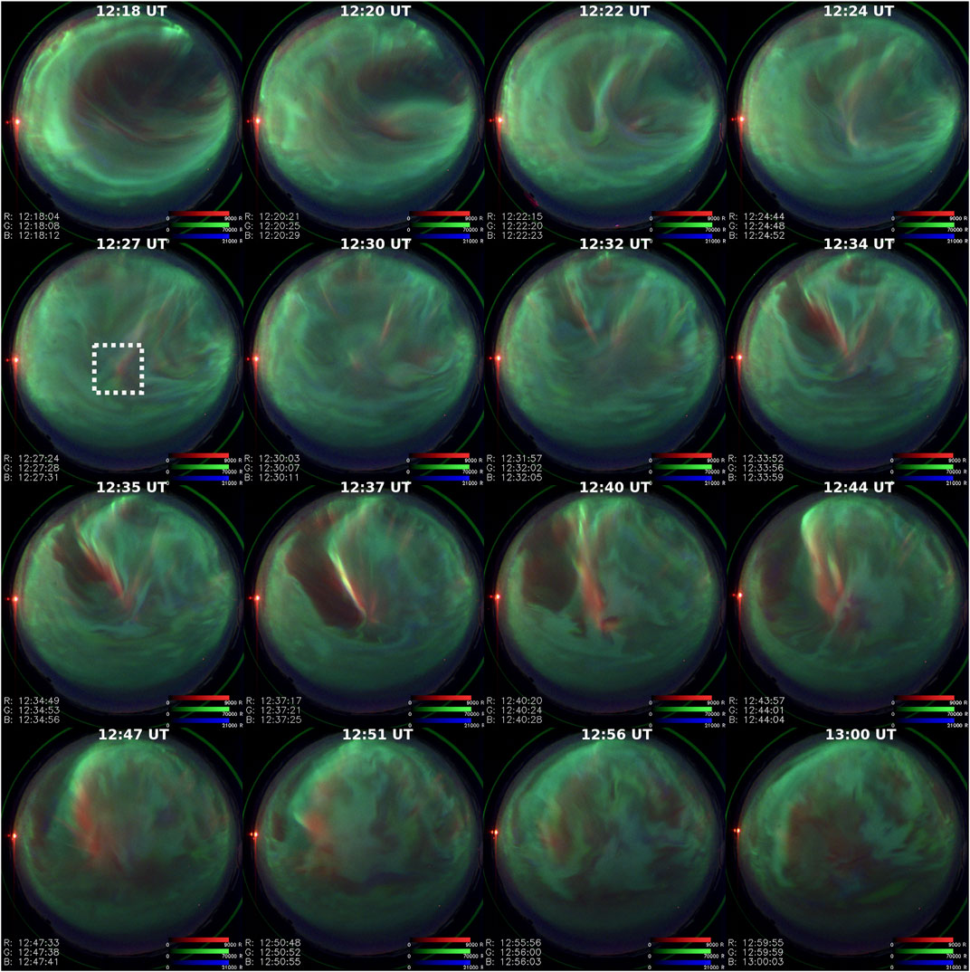
FIGURE 4. Composite (red, green, blue) All Sky Imager frames from the Poker Flat EMCCD. Selected images are not regularly sampled from available data but are meant to depict the evolution of the aurora during the event. In all frames, North is up and East is right. The white, dotted square indicates the location of magnetic zenith (center of the square), which is the same in all frames.

Small, dim red-line features can be seen in the composite images in Figure 4 from 12:20 UT onward. The most notable feature is the sudden appearance of a red-line arc which forms on the boundary of a large region of black aurora. This feature is first apparent in the 12:32 UT frame in Figure 4; though, a weak red-line structure is visible in approximately the same location in the 12:20 UT frame. From ∼ 12:34 to 12:37 UT, the region of black aurora expands to the southwest (towards magnetic zenith). During this, the red-line emission increases in intensity and moves with the black aurora, extending outward from roughly magnetic zenith and stretching northward. At ∼ 12:40 UT, the red-line arc appears to break apart into smaller structures and pulsating patch structures move into the region of black aurora from the south. Bright, green-line features appear to be co-located with the red-line arc. As the black aurora “retreats” westward and eventually disappears or becomes non-distinct, the intensity of the red-line emission diminishes, the arc becomes diffuse, and by the last frame in Figure 4, it is gone.

4 Analysis

Figure 5 shows the pulsating aurora from this event as a time series of the emission brightness. Pulsations are seen as periodic enhancements in the brightness in the 557.7 nm emission-line (shown in green). Figure 5 also includes T_e, N_e, and v_i from Beam 7 as separate panels. In each panel, the data has been averaged over altitude for each time interval. Note that the line-of-sight ion velocities measured by Beam 7 are measurements of ion upflow and downflow, since Beam 7 is oriented along the local magnetic field line. The onset of the red-line enhancement (∼ 12:37 UT; see Figure 4) coincides with the highest magnitude T_e recorded by PFISR in the magnetic zenith look direction during the hour of UT 12, the largest v_i enhancement, and a local minimum in N_e. As T_e decreases, so too does the enhancement in v_i. Concurrently, N_e recovers from the local minimum. These behaviors occur simultaneously with the movement of the red-line enhancement westward (i.e. away from magnetic zenith). It is worth noting that the local peak in red-line emission overlaps with the largest upflow feature. This could be merely coincidental, since the look directions for red-line observations and ion upflow are not common volume. This can be seen by comparing the orientation of Beam 7, which is pointed toward magnetic zenith, to the white box in Figure 4 (also denoting the position of magnetic zenith). There could be a causal relationship between the ion upflow and red-line emission, but it is impossible to say definitively from the optical and radar results alone.

FIGURE 5

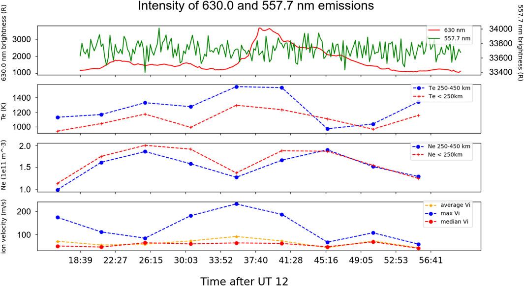
FIGURE 5. Intensity of the 630.0 (red-line) and 557.7 nm (green-line) emission shown together with their respective scales (first panel). The camera pixels used for this time series are an average of the 50 × 50 pixel square indicated in Figure 4. Parameters from PFISR Beam 7 are displayed in the subsequent panels for comparison. In each of these panels, the data has been averaged over altitude for each time interval. Electron temperature is shown in the second panel, with the blue line displaying the average between 250 and 450 km and the red-line the average below 250 km. The third panel shows the same averages for the electron density. The bottom panel shows the ion upflow velocities represented three ways: the maximum value (blue line) the average value (yellow line) and the median value (red line) all within the region between 250 and 450 km.

The first panel of Figure 5 shows the average intensity of the 630.0 and 557.7 nm emission lines, averaged over the 50 × 50 pixel square denoted by the white, dotted box in Figure 4 to obtain the average brightness of the pulsating aurora at magnetic zenith. The second panel shows the T_e averaged in two regions; from 250 to 450 km and below 250 km, while the third panel shows the N_e averages for the same two regions. The fourth panel shows three representations of the v_i in the first region (from 250 to 450 km), as the maximum (blue), average (yellow), and median (red). These three different methods of representation are utilized in order to adequately characterize the velocity enhancement. The overall agreement in the shape of the three lines demonstrates that the behavior is most likely a real feature as opposed to an artifact of averaging, for example. Further, it is worth noting that the maximum v_i shown here appear to be much higher than the mean and median v_i. However, the fact that the mean is higher than median suggests that some subset of the ion population is being accelerated much more efficiently than the whole. This could plausibly be explained by the ambipolar field lifting the top of the ion population at higher altitudes, causing the ions below to then experience a reduced charge separation/ambipolar field.

Electron precipitation is a known driver of both ion upflow and pulsating aurora, though, the energy scales of the electron precipitation in each case are quite different. Nevertheless, the soft electron precipitation that drives Type II ion upflow (i.e. ∼ hundreds of eV), establishes an ambipolar electric field that lifts ions upward [33]. Such an ambipolar electric field was indeed estimated during this event alongside pulsating aurora, and its altitude profile is calculated and shown in Figure 6. This field is calculated as the electron pressure gradient, as defined by Eq. (1), in which N_e is the electron number density, T_e the electron temperature, e the elementary charge, and k_B is Boltzmann’s constant.

$E_{\Vert }=\frac{-1}{e{N}_e}{\nabla }_{\Vert }\left(N_e{k}_B{T}_e\right)=\frac{-k_B}{e}\left[\nabla T_e+T_e\frac{\nabla N_e}{N_e}\right](1)$

FIGURE 6

FIGURE 6. Relevant parameters are shown here for the times indicated (UT). From left to right: electron temperature, electron density, ambipolar electric field, field aligned potential, and ion line-of-sight velocity, with the altitude of the measurement indicated by the y-axis. Data are from the PFISR Beam 7, which is oriented along the local magnetic field line. In panel, the data has been averaged over altitude for each time interval.

The electric potential along the magnetic field line can be calculated as the integral of this ambipolar electric field. This calculation has been performed for each 5 min integration bin of PFISR (Beam 7) data. Figure 6 shows four selected times beginning at 12:36, 12:41, 12:51, and 13:01 UT respectively. The evolution of the ambipolar electric field, (field-aligned) electric potential, and quantities used to derive these values (including the electron temperature, electron number density, and line-of-sight velocity) are shown in the five panels of Figure 6.

The data presented are error filtered to remove points where the measurement error in T_e > 1000 K or ion line-of-sight velocity $>$ 800 m/s, thus eliminating data points where the statistics were too low to achieve acceptable fits to the parameters. The PFISR data beginning at 13:01 UT are displayed preferentially to those at 12:56 UT because this error filtering removes most data above 350 km for the 12:56 UT time integration. The ambipolar field and potentials shown in Figure 6 have been selected to demonstrate the conditions at the start, in the middle, and at the end of this enhanced upflow event.

Figures 5, 6 show a drop in the electric potential at 300 km and upward. The 12:41 UT line (yellow) in the fourth panel of Figure 6 shows the highest magnitude of this potential, reaching a peak of ∼ 0.4 V–roughly twice the potential of the 12:36 UT (blue) and 13:01 UT (red) lines, and coincident with the bulk of the v_i enhancement below 400 km. As is evident in comparing Figures 5, 6, the period of time with the highest v_i signature is not coincident with the with strongest potential drop, though, this offset could in part be an effect of the 5 minute time integration.

Further, we do not expect to observe the maximum ion velocity occurring at the same time and/or location as the maximum value of the ambipolar electric field due to the expected time and space delays between the two parameters. This is due to the fact that the ion velocity is the integral of the acceleration over the history of the flux tube in its convecting frame, which is not the stationary frame of the radar observation in Beam 7.

Quantitatively speaking, in the absence of collisional drag, an electric field of ∼ ± 2.5 × 10^–6 V/m, with a gravitational acceleration of 9.21 m/s² at 200 km altitude would produce a net upwards acceleration on O⁺ ions of ∼ 5.8 m/s². At this acceleration, it would take ∼ 34.5 s to accelerate an O⁺ ion from rest to 200 m/s. If the horizontal velocities are on the order of 500 m/s, then in ∼ 34.5 s, the flux tube would move ∼ 17.2 km horizontally. For comparison, the radar beam is only approximately 5 km wide at 250 km altitude. The inability to fully reconstruct complete flux tube histories in their convecting frames is a longstanding difficulty with the interpretation of ion upflow data from radars.

It is worth noting that the ambipolar electric field strength calculated here (∼ ± 2.5 × 10^–6 V/m) is consistent with the estimated 10^–6 V/m value predicted by Li et al. [50] (and references therein). Meanwhile, the ion upflow velocities that we observe here (∼ ± 250 m/s) are consistent with those observed by Loranc et al. [51] (100–250 m/s between 216 and 400 km), and by Fernandes et al. [29]; and references therein (up to 300 m/s below 325 km on the nightside). Further, the high-altitude (upper F region ionosphere) electron temperatures estimated here (∼ 1000 K), are consistent with the ∼ 500–1000 K electron temperatures reported by Liang et al. [52], during similar transits of pulsating aurora over PFISR.

5 Discussion

The cause of the red-line emission enhancement and associated soft electron precipitation for this case is unknown. On one hand, Alfvén waves are often considered to be a local driver of soft electron precipitation Chaston et al. ([53]; Chaston and Seki [54] and references therein). On the other hand, discrete auroral arcs, such as this red-line feature, are typically associated with potential structures that lead to higher energy electron precipitation; i.e. a non-local source. Perhaps there is another mechanism at play in this case.

Neutral upwelling is a possible source of the observed red-line emission as the chemical red-line production is essentially proportional to the product between the ion and neutral densities. Granted, this mechanism is likely insufficient to account for a 2000 R increase in emission intensity.

Evans et al. [55] presented data from the NOAA 6 satellite and subsequent analysis which demonstrated a consistent, low energy tail in electron spectra in the region of pulsating aurora that they attributed to “backscattered” (also called “secondary”) electrons caused by the “primary” population of high energy electron precipitation in the opposite hemisphere. Recently, Khazanov et al. [56] demonstrated through the use of optical data that such a population of secondary electrons may undergo bounce motion, “subsequently contributing to the total precipitating electron flux in any given hemisphere.” They confirm these results with predictions of the SuperThermal Electron Transport (STET) model, which predicts for such a scenario that 15–40% of the energy flux gets reflected back up for the primary precipitating electrons with energies of 5 keV [57].

The sudden increase in red-line emission (∼ 12:37 to 12:41 UT) implies that there is a localized, lower energy broadband portion of the precipitating electron spectra on the boundary of the black aurora and diffuse/pulsating auroral regions driving the red-line emission. Indeed, the secondary electrons which contribute to the low energy portion of the electron spectrum associated with pulsating aurora [55], appear as periodic, small increases in brightness (i.e. pulsations) in camera data [58]. However, it is unlikely that such secondary electrons produce the sudden, localized increase in red-line emission observed here, as their associated pulsations are not the dominant feature present in the optical data.

Fujii et al. [59] suggested that pulsating aurora is driven by electrons that flow along field-aligned currents (FAC) within a pair of oppositely directed current sheets (producing an ionospheric return current). Fritz et al. [20] observed black aurora acting as a boundary between different pulsating structures, which could be a physically similar process to that outlined by Marklund et al. [23]. If this is indeed the case, then we would expect to see the 630.0 nm red-line enhancement on the boundary between oppositely directed currents, represented by the regions of pulsating aurora and black aurora respectively. In Figure 4, we do indeed see the red-line enhancement manifest on the boundary of the pulsating aurora and black aurora, but are unable to determine whether these two types of aurora necessarily represent oppositely directed currents. It is worth noting that Liang et al. [18] reported observations of a red-line arc within the transition region between an upward-directed FAC and a downward-directed FAC, which could be a similar process to the red-line emission we see here.

Chaston et al. [54] present model results of an ionospheric current sheet. In the scenarios explored, it is shown that the time evolution of the current sheet is governed by Kelvin-Helmholtz and tearing instabilities with transverse FAC gradients. Of particular interest in their modeled scenarios, is the generation of inertial, field-aligned Alfvén waves that flow between oppositely-directed currents. Since Alfvén waves are thought to drive the soft electron precipitation responsible for the red-line emission seen in the ASI camera data, this scenario is consistent with the interpretation of pulsating aurora and black aurora as representing oppositely directed current sheets (between which the red-line emission occurs).

Another possibility is as follows. The electron density must increase in the topside ionosphere (see Section 1.2), for Type II ion upflow to occur. Since the ion upflow observed in this case occurs in the vicinity of pulsating aurora, this increased high-altitude electron density creates a density gradient between the regions of pulsating aurora and black aurora. This in turn may facilitate the breakdown of large-scale Alfvén waves into small-scale inertial Alfvén waves through the process described in Lysak and Song [60]. This mechanism may explain the time delay between the observed ion upflow and red-line emission.

Brambles et al. [61] present a scaling law that relates Poynting (energy) flux and ion outflow (O⁺ flux). It is unclear whether this relationship necessarily indicates a relationship between Alfvén waves and the wave-particle-interactions at high altitudes (which would drive the conversion from ion upflow to ion outflow), or a relationship between Alfvén waves and low-altitude acceleration of ion upflow, or both. It is possible that Alfvén wave excitation contributes to ion upflow if it represents a sufficiently large Poynting flux into the ionosphere. It is unclear, however, whether Alfvén waves are responsible for both the red-line emission and ion upflow observed for this event since the ion upflow signature establishes ∼ 15–20 min prior to the onset of the red-line enhancement (see Figures 4, 5). Then again, the peak in the upflowing ion velocity coincides with the beginning of the red-line enhancement, suggesting a correlation between the two phenomena. The relationship between these two features is currently unclear. It is possible that the bulk upward motion of ions (e.g. ion upflow) contributes to an enhanced ion density at greater scale heights. This in turn would afford a higher recombination rate which would result in the enhanced 630.0 nm emission.

In theory, we could test this hypothesis (that the enhanced red-line emission is driven by recombination) by calculating the expected volume emission rate from the PFISR electron density and MSIS neutral density. However, the particle densities observed during this event may well be insufficient to explain the red line intensities by chemistry alone. Such an analysis is beyond the scope of this study.

6 Summary

The timeline of events reported here is summarized as follows:

1) Diffuse aurora is present in the region before the aurora begins to pulsate at ∼ 12:20 UT. The onset of pulsation is followed by an increase in electron temperature and electron number density (at low altitudes), as shown in Figures 3, 5. The rising “plume” of ionization indicated by the red circle in Figure 3 is likely a signature of Type II ion upflow, which requires an expanding electron gas to create the ambipolar electric field necessary to accelerate ions to higher altitudes.

2) At ∼ 12:30 UT, the line-of-sight ion velocities (Beams 1 and 2, oblique to the local magnetic field) indicate a decrease in the eastward convection signature, while the ion upflow velocities (from Beam 7, oriented along the local magnetic field) increase following pulsation onset. The upflow signature is shown in Figure 2, while the corresponding average (yellow), maximum (blue), and median (red) ion upflow velocities are calculated and shown in Figure 5.

3) Electron pressure gradients establish an ambipolar electric field, calculated and shown in Figure 6. These gradients may be driven by secondary electrons and/or low levels of soft electron precipitation (as evinced by the weak red-line intensity seen in Figure 4 prior to ∼ 12:34 UT).

4) The line-of-sight ion velocities and electron temperature increase to their maximum values while the electron number density up to 450 km decreases to a local minimum (∼ 12:37 UT), as shown in Figure 5. This behavior is consistent with the expansion of electron gas (that produces the charge separation necessary for the establishment of the ambipolar electric field), moving from low altitudes to higher altitudes.

5) Between ∼ 12:37 and 12:40 UT, the intensity of the red-line structure increases abruptly (see Figures 4, 5). The red-line structure then proceeds to follow the boundary of the black aurora region westward.

6) Pulsating aurora drifts into the larger region of black aurora as the black aurora moves westward. The bright structure along the boundary begins to fade and then break apart (between ∼ 12:37 and 12:40 UT).

7) Finally, the red-line enhancement exits the region of magnetic zenith (∼ 12:51 UT), fades, and then disappears from view (∼ 13:00 UT).

We have presented a dataset which demonstrates a localized ion upflow event in conjunction with a localized increase in red-line emission. These events occur after pulsating aurora has existed in the region for ∼ 20–25 min, during which time, eastward convection has diminished. The PFISR data indicate that, during the period of pulsating aurora, T_e and N_e increase and an ambipolar electric field is established.

The largest magnitude ion upflow signature coincides with an abrupt increase in the 630.0 nm emission line. This red-line emission appears as part of a discrete auroral arc on the boundary between a large region of black aurora and pulsating aurora. As the arc drifts westward, it appears to break up and the pulsating aurora drifts into the region of black aurora.

The source of this increase in the red-line emission is currently unknown, but possible drivers are presented and discussed. Electron precipitation associated with Alfvénic aurora is a more likely driver than electron backscatter; which would result in rapidly varying fluctuations in the camera data that we simply do not observe here [58].

Kelvin-Helmholtz, tearing, and Rayleigh-Taylor instabilities have also been proposed as possible drivers of red-line emission [54]. Kelvin-Helmholtz and tearing instabilities are associated with sheared edges and/or vortical formations. From the available camera data, however, there are no clear signs of sheared edges or vortical structures associated with the red-line enhancement (see Figure 4). Rayleigh-Taylor instabilities are a possible driver, though, the camera resolution makes it impossible to definitely determine whether we see the vortical structures associated with Rayleigh-Taylor instabilities in the optical data. Comparisons between ASI observations (e.g. remote) of pulsating aurora and satellite or rocket observations (e.g. in-situ) may be useful in determining the energy and pitch-angle distributions for the low energy electron populations, which the 630.0 nm auroral emission suggest are present.

The sudden appearance of the red-line arc which follows the boundary of black aurora and pulsating aurora regions is an unusual phenomenon that warrants further examination. Further statistical studies should be conducted to investigate the generating mechanism, providing clues to open questions; i.e. Is the topology of the (red-line) arc always N-S aligned? Does it always coincide with ion upflow? Does it happen when convection signatures are present in ISR data? Is the intensity of the arc correlated with the strength of the oppositely-directed currents thought to form the boundary between black aurora and pulsating aurora? Further studies are needed to understand events such as this one.

Data availability statement

The datasets presented in this study can be found in online repositories. The names of the repository/repositories and accession number(s) can be found below: https://data.amisr.com/database/61/experiment/20170205.001/3/ and http://optics.gi.alaska.edu/realtime/data/MPEG/PKR_DASC_256/2017/. These data are publicly available and do not require accession numbers or passwords.

Author contributions

The general experiment concept design and preliminary analysis of results was conducted by BF. Subsequent data analysis, and initial drafting of this manuscript was performed by DK under the guidance of ML Parts of this manuscript have previously appeared in DK's PhD graduate thesis. NG has been involved with the science discussions related to this manuscript since its early stages, and has reworked the majority of the text into its current form under the guidance of ML Figure 1 was provided by NG and is based on the TopsideUpflow2 overview plot created by created by RV, publicly available on the Advanced Modular Incoherent Scatter Radar database (URL: https://data.amisr.com/database/61/experiment/20170205.001/3/). Figures 2 and 3 were provided by RV. Figure 4 was created by DK, using composite all-sky imager data provided by DH (available at: http://optics.gi.alaska.edu/realtime/data/MPEG/PKR_DASC_256/2017/). Figures 5 and 6 were provided by DK.

Funding

This work is supported at the University of New Hampshire by NASA grants 80NSSC18K0965, NNX17A138G, NNX13AJ94G, and NNH20ZDA001N-FINESST. This material is based upon work supported by the Poker Flat Incoherent Scatter Radar which is a major facility funded by the National Science Foundation through cooperative agreement AGS-1840962 to SRI International. BF is supported by the Office of Naval Research.

Acknowledgments

Data analysis and initial drafting of this manuscript was performed by DK under the guidance of ML. Parts of this manuscript have previously appeared in [60], as part of DK‘s PhD graduate thesis. NG would like to thank the undergraduate and graduate student researchers, faculty, and staff of the Magnetosphere-Ionosphere Research Laboratory at the University of New Hampshire for their input and scientific expertise. Further, we would like to thank all of our friends, colleagues, and collaborators at each of their respective institutions for their ongoing support and guidance. The process of conducting research is seldom a straightforward one even during the best of times. Although the COVID-19 pandemic has presented us all with many challenges, the grace and resilience with which our friends and colleagues continue to adapt and persevere despite these difficult circumstances is admirable.

Conflict of interest

The authors declare that the research was conducted in the absence of any commercial or financial relationships that could be construed as a potential conflict of interest.

Publisher’s note

All claims expressed in this article are solely those of the authors and do not necessarily represent those of their affiliated organizations, or those of the publisher, the editors and the reviewers. Any product that may be evaluated in this article, or claim that may be made by its manufacturer, is not guaranteed or endorsed by the publisher.

Supplementary material

The Supplementary Material for this article can be found online at: https://www.frontiersin.org/articles/10.3389/fphy.2022.997229/full#supplementary-material

Supplementary Video S1 | Composite (red, green, blue) All Sky Imager footage from the Poker Flat EMCCD, for the February 5th, 2017 event described in this manuscript. Individual frames from this video were selected to demonstrate the evolution of the pulsating aurora, black aurora, and red-line feature shown in Figure 4.

References

1. Liang J, Yang B, Donovan E, Burchill J, Knudsen D. Ionospheric electron heating associated with pulsating auroras: A swarm survey and model simulation. J Geophys Res Space Phys (2017) 122:8781–807. doi:10.1002/2017JA024127

CrossRef Full Text | Google Scholar

2. Jones SL, Lessard MR, Rychert K, Spanswick E, Donovan E, Jaynes AN. Persistent, widespread pulsating aurora: A case study. JGR Space Phys (2013) 118:2998–3006. doi:10.1002/jgra.50301

CrossRef Full Text | Google Scholar

3. Partamies N, Whiter D, Kadokura A, Kauristie K, Nesse Tyssøy H, Massetti S, et al. Occurrence and average behavior of pulsating aurora. J Geophys Res Space Phys (2017) 122:5606–18. doi:10.1002/2017JA024039

CrossRef Full Text | Google Scholar

4. Akasofu S.∼I. Polar and Magnetosphere Substorms (1968) 11. Springer Dordrecht. doi:10.1007/978-94-010-3461-6

CrossRef Full Text | Google Scholar

5. Duthie DD, Scourfield MWJ. Aurorae and closed magnetic field lines. J Atmos Terrestrial Phys (1977) 39:1429–34. doi:10.1016/0021-9169(77)90099-X

CrossRef Full Text | Google Scholar

6. Oguti T, Kokubun S, Hayashi K, Tsuruda K, Machida S, Kitamura T, et al. Statistics of pulsating auroras on the basis of all-sky TV data from five stations. I. Occurrence frequency. Can J Phys (1981) 59:1150–7. doi:10.1139/p81-152

CrossRef Full Text | Google Scholar

7. Royrvik O, Davis TN. Pulsating aurora: Local and global morphology. J Geophys Res (1977) 82:4720–40. doi:10.1029/JA082i029p04720

CrossRef Full Text | Google Scholar

8. Humberset BK, Gjerloev JW, Samara M, Michell RG, Mann IR. Temporal characteristics and energy deposition of pulsating auroral patches. J Geophys Res Space Phys (2016) 121:7087–107. doi:10.1002/2016JA022921

CrossRef Full Text | Google Scholar

9. Jones SL, Lessard MR, Rychert K, Spanswick E, Donovan E. Large-scale aspects and temporal evolution of pulsating aurora. J Geophys Res (2011) 116. doi:10.1029/2010JA015840

CrossRef Full Text | Google Scholar

10. Newell PT, Sotirelis T, Wing S. Diffuse, monoenergetic, and broadband aurora: The global precipitation budget. J Geophys Res (2009) 114. doi:10.1029/2009JA014326

CrossRef Full Text | Google Scholar

11. Brown NB, Davis TN, Hallinan TJ, Stenbaek-Nielsen HC. Altitude of pulsating aurora determined by a new instrumental technique. Geophys Res Lett (1976) 3:403–4. doi:10.1029/GL003i007p00403

CrossRef Full Text | Google Scholar

12. Kasahara S, Miyoshi Y, Yokota S, Mitani T, Kasahara Y, Matsuda S, et al. Pulsating aurora from electron scattering by chorus waves. Nature (2018) 554:337–40. doi:10.1038/nature25505

PubMed Abstract | CrossRef Full Text | Google Scholar

13. Miyoshi Y, Oyama S, Saito S, Kurita S, Fujiwara H, Kataoka R, et al. Energetic electron precipitation associated with pulsating aurora: EISCAT and van allen probe observations. J Geophys Res Space Phys (2015) 120:2754–66. doi:10.1002/2014JA020690

CrossRef Full Text | Google Scholar

14. Solomon SC, Hays PB, Abreu VJ. The auroral 6300 Å emission: Observations and modeling. J Geophys Res (1988) 93:9867–82. doi:10.1029/JA093iA09p09867

CrossRef Full Text | Google Scholar

15. Link R, Cogger LL. A reexamination of the o i 6300-Å nightglow. J Geophys Res (1988) 93:9883–92. doi:10.1029/JA093iA09p09883

CrossRef Full Text | Google Scholar

16. Eather RH. Short-period auroral pulsations in λ 6300 O_I. J Geophys Res (1896) 74:4998–5004. doi:10.1029/JA074i021p04998

CrossRef Full Text | Google Scholar

17. Liang J, Donovan E, Jackel B, Spanswick E, Gillies M. On the 630 nm red-line pulsating aurora: Red-line Emission Geospace Observatory observations and model simulations. J Geophys Res Space Phys (2016) 121:7988–8012. doi:10.1002/2016JA022901

CrossRef Full Text | Google Scholar

18. Liang J, Shen Y, Knudsen D, Spanswick E, Burchill J, Donovan E. e-pop and red line optical observations of alfvénic auroras. J Geophys Res Space Phys (2019) 124:4672–96. doi:10.1029/2019JA026679

CrossRef Full Text | Google Scholar

19. Gillies MD, Knudsen D, Donovan E, Jackel B, Gillies R, Spanswick E. Identifying the 630 nm auroral arc emission height: A comparison of the triangulation, fac profile, and electron density methods. J Geophys Res Space Phys (2017) 122:8181–97. doi:10.1002/2016JA023758

CrossRef Full Text | Google Scholar

20. Fritz BA, Lessard MR, Blandin MJ, Fernandes PA. Structure of black aurora associated with pulsating aurora. JGR Space Phys (2015) 120:10096–106. doi:10.1002/2015JA021397

CrossRef Full Text | Google Scholar

21. Peticolas LM, Hallinan TJ, Stenbaek-Nielsen HC, Bonnell JW, Carlson CW. A study of black aurora from aircraft-based optical observations and plasma measurements on FAST. J Geophys Res (2002) 107:SMP 30-1–SMP 30-11. doi:10.1029/2001JA900157

CrossRef Full Text | Google Scholar

22. Sakaguchi K, Shiokawa K, Donovan E, Nakajima A, Hiraki Y, Trondsen T, et al. Periodic black auroral patches at the dawnside dipolarization front during a substorm. J Geophys Res (2011) 116. doi:10.1029/2010JA015957

CrossRef Full Text | Google Scholar

23. Marklund G, Karlsson T, Clemmons J. On low-altitude particle acceleration and intense electric fields and their relationship to black aurora. J Geophys Res (1997) 102:17509–22. doi:10.1029/97JA00334

CrossRef Full Text | Google Scholar

24. Nishimura Y, Lessard MR, Katoh Y, Miyoshi Y, Grono E, Partamies N, et al. Diffuse and pulsating aurora. Space Sci Rev (2020) 216:4. doi:10.1007/s11214-019-0629-3

CrossRef Full Text | Google Scholar

25. Chen SH, Boardsen SA, Fung SF, Green JL, Kessel RL, Tan LC, et al. Exterior and interior polar cusps: Observations from Hawkeye. J Geophys Res (1997) 102:11335–47. doi:10.1029/97JA00743

CrossRef Full Text | Google Scholar

26. Chen J, Fritz TA, Sheldon RB, Spence HE, Spjeldvik WN, Fennell JF, et al. Cusp energetic particle events: Implications for a major acceleration region of the magnetosphere. J Geophys Res (1998) 103:69–78. doi:10.1029/97JA02246

CrossRef Full Text | Google Scholar

27. Liu H, Ma SY, Schlegel K. Diurnal, seasonal, and geomagnetic variations of large field-aligned ion upflows in the high-latitude ionospheric F region. J Geophys Res (2001) 106:24651–61. doi:10.1029/2001JA900047

CrossRef Full Text | Google Scholar

28. Ogawa Y, Buchert SC, Fujii R, Nozawa S, van Eyken AP. Characteristics of ion upflow and downflow observed with the European incoherent scatter svalbard radar. J Geophys Res (2009) 114. doi:10.1029/2008JA013817

CrossRef Full Text | Google Scholar

29. Fernandes PA, Lynch KA, Zettergren M, Hampton DL, Bekkeng TA, Cohen IJ, et al. Measuring the seeds of ion outflow: Auroral sounding rocket observations of low-altitude ion heating and circulation. JGR Space Phys (2016) 121:1587–607. doi:10.1002/2015JA021536

CrossRef Full Text | Google Scholar

30. Ren J, Zou S, Lu J, Giertych N, Chen Y, Varney RH, et al. Statistical study of ion upflow and downflow observed by PFISR. JGR Space Phys (2020) 125:e2020JA028179. doi:10.1029/2020JA028179

CrossRef Full Text | Google Scholar

31. Yau AW, André M. Sources of ion outflow in the high latitude ionosphere. Space Sci Rev (1997) 80:1–25. doi:10.1023/A:1004947203046

CrossRef Full Text | Google Scholar

32. Wahlund JE, Opgenoorth HJ, Haggstrom I, Winser KJ, Jones GOL. EISCAT observations of topside ionospheric ion outflows during auroral activity: Revisited. J Geophys Res (1992) 97:3019–37. doi:10.1029/91JA02438

CrossRef Full Text | Google Scholar

33. Strangeway RJ, Ergun RE, Su YJ, Carlson CW, Elphic RC. Factors controlling ionospheric outflows as observed at intermediate altitudes. J Geophys Res (2005) 110:A03221. doi:10.1029/2004JA010829

CrossRef Full Text | Google Scholar

34. Skjæveland A, Moen J, Carlson HC. On the relationship between flux transfer events, temperature enhancements, and ion upflow events in the cusp ionosphere. J Geophys Res (2011) 116. doi:10.1029/2011JA016480

CrossRef Full Text | Google Scholar

35. Skjæveland A, Moen J, Carlson HC. Which cusp upflow events can possibly turn into outflows? J Geophys Res Space Phys (2014) 119:6876–90. doi:10.1002/2013JA019495

CrossRef Full Text | Google Scholar

36. Dubinin E, Lundin R. Mass-loading near mars. Adv Space Res (1995) 16:75–9. doi:10.1016/0273-1177(95)00211-V

CrossRef Full Text | Google Scholar

37. Sandhu JK, Yeoman TK, Rae IJ, Fear RC, Dandouras I. The dependence of magnetospheric plasma mass loading on geomagnetic activity using Cluster. J Geophys Res Space Phys (2017) 122:9371–95. doi:10.1002/2017JA024171

CrossRef Full Text | Google Scholar

38. Winglee RM, Chua D, Brittnacher M, Parks GK, Lu G. Global impact of ionospheric outflows on the dynamics of the magnetosphere and cross-polar cap potential. J Geophys Res (2002) 107:1237. doi:10.1029/2001JA000214

CrossRef Full Text | Google Scholar

39. Yau AW, Howarth A, Peterson WK, Abe T. Transport of thermal-energy ionospheric oxygen (O⁺) ions between the ionosphere and the plasma sheet and ring current at quiet times preceding magnetic storms. J Geophys Res (2012) 117:A07215. doi:10.1029/2012JA017803

CrossRef Full Text | Google Scholar

40. Denton RE, Takahashi K, Thomsen MF, Borovsky JE, Singer HJ, Wang Y, et al. Evolution of mass density and O+ concentration at geostationary orbit during storm and quiet events. JGR Space Phys (2014) 119:6417–31. doi:10.1002/2014JA019888

CrossRef Full Text | Google Scholar

41. Denton RE, Thomsen MF, Takahashi K, Anderson RR, Singer HJ. Solar cycle dependence of bulk ion composition at geosynchronous orbit. J Geophys Res (2011) 116:A03212. doi:10.1029/2010JA016027

CrossRef Full Text | Google Scholar

42. Takahashi K, Denton RE, Singer HJ. Solar cycle variation of geosynchronous plasma mass density derived from the frequency of standing Alfvén waves. J Geophys Res (2010) 115:A07207. doi:10.1029/2009JA015243

CrossRef Full Text | Google Scholar

43. Berube D, Moldwin MB, Ahn M. Computing magnetospheric mass density from field line resonances in a realistic magnetic field geometry. J Geophys Res (2006) 111:A08206. doi:10.1029/2005JA011450

CrossRef Full Text | Google Scholar

44. Fraser BJ, Horwitz JL, Slavin JA, Dent ZC, Mann IR. Heavy ion mass loading of the geomagnetic field near the plasmapause and ULF wave implications. Geophys Res Lett (2005) 32:L04102. doi:10.1029/2004GL021315

CrossRef Full Text | Google Scholar

45. Lessard MR, Lindgren EA, Engebretson MJ, Weaver C. Solar cycle dependence of ion cyclotron wave frequencies. J Geophys Res Space Phys (2015) 120:4711–8. doi:10.1002/2014JA020791

CrossRef Full Text | Google Scholar

46. Denton RE, Jordanova VK, Fraser BJ. Effect of spatial density variation and O+ concentration on the growth and evolution of electromagnetic ion cyclotron waves. JGR Space Phys (2014) 119:8372–95. doi:10.1002/2014JA020384

CrossRef Full Text | Google Scholar

47. Lee DH, Johnson JR, Kim K, Kim KS. Effects of heavy ions on ULF wave resonances near the equatorial region. J Geophys Res (2008) 113:A11212. doi:10.1029/2008JA013088

CrossRef Full Text | Google Scholar

48. Lynch KA, Hampton DL, Zettergren M, Bekkeng TA, Conde M, Fernandes PA, et al. MICA sounding rocket observations of conductivity-gradient-generated auroral ionospheric responses: Small-scale structure with large-scale drivers. JGR Space Phys (2015) 120:9661–82. doi:10.1002/2014JA020860

CrossRef Full Text | Google Scholar

49. Kamide Y, Vickrey JF. Variability of the Harang discontinuity as observed by the Chatanika radar and the IMS Alaska magnetometer chain. Geophys Res Lett (1983) 10:159–62. doi:10.1029/GL010i002p00159

CrossRef Full Text | Google Scholar

50. Li K, Haaland S, Wei Y. A new concept to measure the ambipolar electric field driving ionospheric outflow. J Geophys Res Space Phys (2021) 126:e2020JA028409. doi:10.1029/2020JA028409

CrossRef Full Text | Google Scholar

51. Loranc M, Hanson WB, Heelis RA, St-Maurice JP. A morphological study of vertical ionospheric flows in the high-latitude F region. J Geophys Res (1991) 96:3627. doi:10.1029/90JA02242

CrossRef Full Text | Google Scholar

52. Liang J, Donovan E, Reimer A, Hampton D, Zou S, Varney R. Ionospheric electron heating associated with pulsating Auroras: Joint optical and PFISR observations. J. Geophys. Res. Space Phys. (2018) 123 (5), 4430–4456. doi:10.1029/2017JA025138

CrossRef Full Text | Google Scholar

53. Chaston CC, Carlson CW, Peria WJ, Ergun RE, McFadden JP. FAST observations of inertial alfven waves in the dayside aurora. Geophys Res Lett (2001) 26:647–50. doi:10.1029/1998GL900246

CrossRef Full Text | Google Scholar

54. Chaston CC, Seki K. Small-scale auroral current sheet structuring. J Geophys Res (2010) 115. doi:10.1029/2010JA015536

CrossRef Full Text | Google Scholar

55. Evans DS, Davidson GT, Voss HD, Imhof WL, Mobilia J, Chiu YT. Interpretation of electron spectra in morningside pulsating aurorae. J Geophys Res (1987) 92:12295–306. doi:10.1029/JA092iA11p12295

CrossRef Full Text | Google Scholar

56. Khazanov GV, Sibeck DG, Zesta E. Is diffuse aurora driven from above or below? Geophys Res Lett (2017) 44:641–7. doi:10.1002/2016GL072063

CrossRef Full Text | Google Scholar

57. Khazanov GV, Glocer A, Himwich EW. Magnetosphere-ionosphere energy interchange in the electron diffuse aurora. J Geophys Res Space Phys (2014) 119:171–84. doi:10.1002/2013JA019325

CrossRef Full Text | Google Scholar

58. Samara M, Michell RG, Khazanov GV. First optical observations of interhemispheric electron reflections within pulsating aurora. Geophys Res Lett (2017) 44:2618–23. doi:10.1002/2017gl072794

CrossRef Full Text | Google Scholar

59. Fujii R, Oguti T, Yamamoto T. Relationships between pulsating auroras and field-aligned electric currents, 36. National Institute Polar ResearchMemoirs (1985)

Google Scholar

60. Lysak RL, Song Y. Propagation of kinetic Alfvén waves in the ionospheric Alfvén resonator in the presence of density cavities. Geophys. Res. Lett. (2008) 35 (20). doi:10.1029/2008GL035728

CrossRef Full Text | Google Scholar

61. Brambles OJ, Lotko W, Zhang B, Wiltberger M, Lyon J, Strangeway RJ. Magnetosphere sawtooth oscillations induced by ionospheric outflow. Science (2011) 332:1183–6. doi:10.1126/science.1202869

PubMed Abstract | CrossRef Full Text | Google Scholar