 Malcolm J. Morrison
 A. Claire Gahagan
- Ottawa Research and Development Centre, Agriculture and Agri-Food Canada, Ottawa, ON, Canada
Future crop varieties must be higher yielding, stress resilient and climate agile to feed a larger population, and overcome the effects of climate change. This will only be achieved by a fusion of plant breeding with multiple “omic” sciences. Field-based, proximal phenomics assesses plant growth and responses to stress and agronomic treatments, in a given environment, over time and requires instruments capable of capturing data, quickly and reliably. We designed the PlotCam following the concepts of cost effective phenomics, being low-cost, light-weight (6.8 kg in total) and portable with rapid and repeatable data collection at high spatial resolution. The platform consisted of a telescoping, square carbon fiber unipod, which allowed for data collection from many heights. A folding arm held the sensor head at the nadir position over the plot, and an accelerometer in the arm ensured the sensor head was level at the time of data acquisition. A computer mounted on the unipod ran custom software for data collection. RGB images were taken with an 18 MP, WiFi controlled camera, infrared thermography data was captured with a 0.3 MP infrared camera, and canopy height measured with a 0.3 MP stereo depth camera. Incoming light and air temperature were logged with every image. New operators were quickly trained to gather reliable and repeatable data and an experienced operator could image up to 300 plots per hour. The PlotCam platform was not limited by field design or topography. Multiple identical PlotCams permitted the study of larger populations generating phenomic information useful in variety improvement. We present examples of data collected with the PlotCam over field soybean experiments to show the effectiveness of the platform.
1 Introduction
Higher yielding, stress resilient crop varieties are a necessity to feed an ever increasing population and overcome the effects of climate change [1–3]. This will only be achieved by a synergy of plant breeding with multiple “omic” sciences. While the advances in sequencing technology have made a plant genome increasingly accessible to science, our capacity to physically describe a plant’s architecture and physiology has not kept pace [3]. Phenomics assesses plant growth, in a given environment, over time [2]. High-throughput phenotyping characterizes large populations of plants rapidly and precisely to eliminate the bottleneck of linking physical traits to genomic sequences [4]. Strategically planned measurements over the course of the growing season, give a clearer representation of a plant’s response to the environment and identify critical periods of development and key physiological attributes linked to a crop’s resilience to stress and subsequent yield.
Field-based, proximal phenomics instruments are used to collect data on crop variety performance under varying environmental conditions [3]. Data collection must be rapid, repeatable, and precise to reliably capture crop changes over time. High spatial resolution is key in the identification of novel phenomic traits and the instrument should also allow the evaluation of large populations of plants (hundreds to thousands) over short intervals.
There are a wide range of field phenomic platforms used to capture image and sensor data. They can be broadly categorized into high clearance tractors [5], manual and power assisted carts [6–8], unmanned aerial vehicles [9] kites and blimps [10], track mounted scanning systems [11] and instrument packages suspended by wires (G [12]). In addition, some have developed relatively low costs systems of cameras and sensors attached to tablets, laptops or data loggers [13].
All phenomic platforms have their inherent advantages and disadvantages. For example, UAVs can image many plots in a very short period of time but can be limited by payload capacity, spatial resolution, flight time and the regulations governing their operation. Carts and high clearance tractors may require transportation infrastructure, have specific plot size requirements, can be limited by crop height, and can result in intra-plot soil compaction. Field scanalyzer systems, while providing highly detailed phenomic information, are costly, subject to high winds and lightning strikes, and being permanently mounted in the field, can lead to soil fatigue and problems with crop rotation. The choice of a phenomics platform should be governed by the crop, the trait of interest, the requirements of the experimental plot design, the expertise of the operator, and the amount of time that can be devoted to post data collection processing [14].
As the costs of sensors, cameras, computers, and electronic components has decreased and their resolution and reliability has increased, the concept of cost effective phenotyping has become more of a reality [14]. Using smaller, lightweight, portable devices may increase the number of locations where phenomics can be done and reduce the specific plot dimension requirements for many proximal platforms. When designing handheld devices, operator fatigue, and skill to choose representative regions of interest in a plot should be considered.
The science of phenomics is still in development and it is important to describe new instrumentation ideas for data collection. To that end, the objective of our manuscript was to describe the features of the PlotCam, a low cost, portable, hand-held field phenomics platform.
2 Materials and methods
2.1 PlotCam structure
The goal when designing the PlotCam was to make an instrument that could support several cameras and sensors at one time, was compact enough to fit on the back seat of a vehicle, and was easily and rapidly assembled once the operator got to the experimental location. The system needed to be light weight to minimize operator fatigue when it was carried from plot to plot. The unipod of the PlotCam, supporting the sensor arm, was constructed from two pieces of hollow, square stock carbon fiber (26 by 26 mm ID Clearwater composites, Deluth MN, United States). The top and bottom pieces, which came apart to facilitate transport, were 940 and 840 mm long, respectively (Figure 1A). The top portion of the unipod contained another piece of square, hollow carbon fiber (20 by 20 mm OD) that telescoped from the larger portion to adjust the height of the sensors. The sensor arm was a rectangular piece of carbon fiber (52 by 26 mm ID and 390 mm long) with a hinge at the joint which allowed the sensor arm to be folded back over the leg of the unipod. For ease of transport, the instrument was designed to conveniently fit into the trunk of a vehicle with the unipod disassembled into the top and bottom sections, and the sensor arm folded over the unipod leg (Figure 1B).
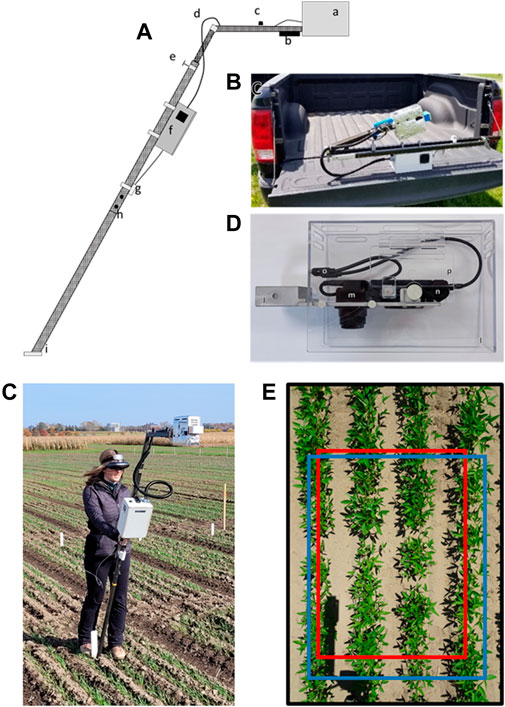
FIGURE 1. (A), Schematic of the PlotCam: a) camera head, b) depth camera, c) pyronometer, d) cabling, e) compression fitting adjustable telescopic pole, f) instrument box, g) temperature sensor, h) joint between upper and lower unipod segments, i) foot mounted at 60o; (B), image of PlotCam folded for transport; (C), Image of operator holding the camera in the field showing the headset and battery belt; (D), Camera head without heat shield covering: j) mounting bracket, k) camera mounting plate, l) plexiglass protective housing, m) infrared camera, n) visible camera, o) internal USB cables to external ports, p) access door, (E) Overlay of the fields of view of the RGB camera (black border, 255 cm × 175 cm dimensions on the ground), depth camera (blue border, 187 cm; 135 cm), and infrared camera (red border, 170 cm × 118 cm) at a PlotCam height of 184 cm.
All of the joints connecting the pieces of carbon fiber were reinforced with square stock hollow aluminum that was milled to fit snugly inside the carbon fiber of the PlotCam unipod. The foot of the unipod was constructed from a piece of flat stock aluminum connected to a piece of square stock and fixed at a 60o angle. When the sensor arm was unfolded and locked in place, and the angled foot of the unipod placed flat on the ground, the cameras were positioned at nadir over the plot (Figures 1A, C).
A short wooden picket, placed in the centre of a field plot adjacent to the range-way provided a marker for the operator to align the foot of the PlotCam, ensuring that the sample area remained consistent on a temporal basis (Figure 1C). When the aluminum foot was placed against the wooden picket and the sensor head placed at a nadir position over the plot, sensor height could be adjusted between 1.6 to 2.2 m above the plot.
To protect the cameras they were mounted in a removable camera head made from a milled piece of aluminum block that fit into the end of the rectangular carbon fiber sensor arm and was attached to a piece of flat stock aluminum (5 mm thick × 70 w × 180 L mm) with cut outs and mounting brackets that kept the cameras level with the sensor arm and in the nadir position (Figure 1D). The camera head was held to the sensor arm with a clip pin that went through the arm and the aluminum block. To shade and protect the instruments, a 3 mm thick Plexiglas housing (78 w × 180 L × 160 h mm) fit over the camera mounting plate attached with four thumb screws. The housing was covered in 5 mm thick aluminum bubble heat shield (Cool Shield, Granger, Can.). A hinged access door on the side of the housing allowed the operator access to the cameras.
2.2 Computer, cameras, and sensors
An instrument box mounted on the unipod, housed an Intel® I5 NUC computer (NUC5i5RYK, Intel, Santa Clara, CA United States), with a 524 GB solid state drive which ran Windows 10 OS and the PlotCam software (Figure 2). The computer had 4 USB ports and an HDMI port. To increase the number of USB ports, two 4-way USB hubs were connected to the computer. USB devices included a wireless handheld trackball mouse (EIGIS 2.4 G Air Mouse, China), a type-K thermocouple mounted on a USB board (Phidget 1051, Calgary, Canada), and an accelerometer (Phidget 1041). The other USB hub was used to power the 18 MP RGB camera (Sony DSC-HX90V, FOV 70o x 50o, Sony, Canada) an external USB port mounted on the outside of the instrument box, a 0.3 MP stereo depth camera (Intel RealSense D415 FOV, 69o × 42o, Intel, Santa Clara, CA, United States) and a pyranometer (Apogee SP215SS, Apogee Instruments, Logan, UT, United States) interfaced via a USB interface board (Phidget Interface Kit 2/2/2). The 0.3 MP infrared camera (ICI 9640, FOV 50o x 40o, ICI - Beaumont, TX United States) was connected to a USB port on the computer. The RGB, infrared and depth cameras were positioned in the head so that the fields of view overlapped facilitating segmentation (Figure 1E). When the height of the sensor arm was changed to accommodate different plot widths the images scaled without changing the overall relative layout.
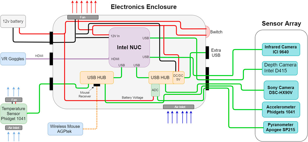
FIGURE 2. Schematic of the PlotCam instrument box.
A 12.8 V 5Ah lithium iron phosphate battery (LiFePO4, RELi3ON relionbattery.com, Rock Hill United States) carried in a utility belt by the operator powered the PlotCam (Figure 1C). An HDMI headset was used to view the computer display, interact with the custom PlotCam software as well as view a live video feed through the RGB camera. Other sensors and plot metadata were managed using the wireless mouse and an on-screen keyboard. The operator could see enough through the bottom of the headset to navigate around the field plots and place the camera in the plot with the unipod foot against the wooden picket. At 6.8 kg in total weight, the PlotCam was optimised to reduce operator fatigue.
2.3 PlotCam software
The PlotCam operating software was written in Visual Basic.net (VB, Microsoft, WA United States). We chose Visual Basic primarily because of the availability of application program interfaces (APIs) and software development kits (SDK) written for the RGB, depth and infrared (IR) cameras and the Phidget devices as well as the ease of creating a graphical user interface in VB.net. The Sony RGB “Camera Remote API” the Intel D415 depth camera (Realsense SDK 2.0) and the ICI 9640 IR camera (ICIx64 SDK) were incorporated into our software and facilitated camera control and data collection. Software development was an evolutionary process with modules added as the camera grew in sensor number and complexity.
The PlotCam software had a main graphic user interface window, two additional windows and two dialog boxes. On start-up, the main window showed connection status of the peripheral devices including; the accelerometer, the light sensor, the air temperature (AT) sensor, the battery voltage, and the zoom percentage of the RGB camera (Figure 3). Live feed was available from the AT and light sensors, the D415 depth camera, and a live video feed through the RGB camera. The operator used this information to check all of the sensor and camera status on start-up and throughout operation.
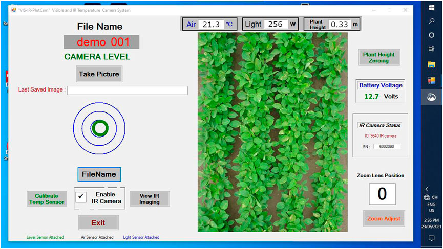
FIGURE 3. View of the main screen of the PlotCam user interface as seen through the headset worn by the operator.
The D415 depth camera initiated at start-up. The operator could set the distance to the ground over a flat surface by activating a depth camera dialog box using the “Plant Height Zeroing” button. This process was done in the lab over a flat surface, based on the width dimension of the plots used for imaging. The telephoto zoom on the Sony camera could be adjusted with the “Zoom Adjust” dialog box and the air temperature sensor was calibrated with the “Calibrate Temp Sensor” dialog box.
A check box on the main window activated the IR camera and brought up the IR camera popup reminding the operator to conduct a non-uniformity correction. To ensure the IR camera was in focus, the “View IR Imaging” button opened a window to view a live video feed, permitting manual focus of the camera as necessary.
The “FileName” button activated an onscreen keyboard window used to enter the metadata required to identify the plot details including the experiment name, day of the year, and plot number. The accelerometer, represented on the main screen by a green “bullseye” floating in blue target rings (Figure 3), was mounted in the sensor arm.
2.4 Operations
Field topology is a necessary consideration when choosing research sites for phenomics. While the integrated accelerometer and design of the PlotCam ensured the that the cameras were maintained at the nadir angle, in cases of extreme topography, such as hills, additional post-processing may be required.
To collect phenomic data on a plot, the operator placed the unipod foot in line with the wooden stake bisecting the plot (Figure 1C), used the RGB video image of the plot displayed on the HDMI headset to centre the image within the plot, and by slight adjustments of the angle of the unipod leg aligned the green circle in the middle of the blue accelerometer target (Figure 3). Once the plot was properly aligned, and the bullseye centered on the accelerometer circles, the operator clicked “Take Picture.” The software required the accelerometer to be centred prior to initiating data capture. After data capture had been initiated the Sony 18 MP RGB image was taken and stored to the camera secure data (SD) card in JPEG format, the D415 image (0.32 MP) was stored to the computer solid state drive in JPEG format, and the D415 depth and IR camera T profiles were each stored in linear arrays in a tab separated text file format. Simultaneously, air T, incoming light, the time stamp, an instantaneous estimate of average height and the camera meta data were stored to a text file along with the image name on the memory card and the plot identifiers entered by the operator. Once all of the data was stored (approximately 2 s), an audible beep informed the operator to move to the next plot. The plot number in the metadata was automatically increased by one. In the case of mistakes the operator could simply re-enter the plot identifier using the “FileName” button, retake the photo and continue.
2.5 Data management, image analysis and data processing
Naming structure was optimized within the system to limit the possibility of data being overwritten or lost. The Sony HX90V camera has limited flexibility in naming structure, so the images were named in series on the memory card. The name as stored on the memory card was obtained from the camera and written to the corresponding line of the tab-delimited text file from that image. The D415 RGB image, the depth array file, and the IR T array file were named using a letter to define the data type (V for RGB, D for depth, and I for infrared), were named using a letter prefix to define the data type (v for RGB, D for depth, and I for infrared), the name of the Sony HX90V image in the memory card, the experiment, the date and the plot number. Files from the PlotCam computer were transferred to working drives using external hard drives, while the images from the Sony RGB camera were transferred by direct USB connection. The downstream analysis of image and sensor data was done using scripts written in Python v.3.8 [15].
Plot RGB images were segmented using a multi-feature machine learning model [16], which output the vegetative cover (VC) (plant pixels/total pixels) for each image based on distinguishing crop pixels from background pixels in the image. Plot IR arrays were segmented using a script based on this algorithm. The IR arrays were overlaid on the RGB images and the non-crop T were removed from the array. The physical location of the cameras on the sensor head (Figure 1D) was such that the IR camera field of view fell within the Sony RGB image field of view to facilitate segmentation as can be seen in Figures 4A, E. The remaining canopy temperatures (CT) were saved as a CSV file that was imported into a Python script to calculate average CT. The air T (AT) was measured every time an IR T was saved. The average CT per plot were normalized by subtracting AT from each plot (CT-AT).
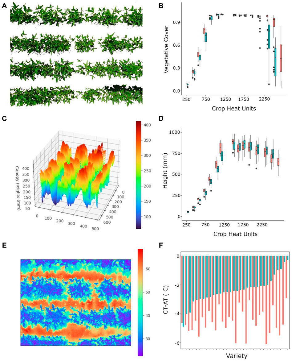
FIGURE 4. Image data types captured by the PlotCam and their corresponding output data; (A) segmented RGB image (2545 mm × 1740 mm), (B) irrigated (red) and non-irrigated (blue) vegetative cover box plots over time showing the median, 25th and 75th percentiles, and outliers from 32 soybean cultivars, (C) a colorized canopy surface height profile (1870 mm × 1440 mm, horizontal axes are pixel coordinates), (D) canopy HT over time paired box plots for irrigated and non-irrigated varieties, (E) infrared thermography colour representation of a soybean canopy (colour scale in Co, 1700 mm × 1180 mm), (F) a comparison of average canopy temperature air temperature difference (CT-AT) for irrigated (red) and non-irrigated (blue) soybean varieties sorted from non-irrigated low to high CT-AT differential.
To calculate plant height (HT) we used the methodology described in Morrison et al. [17]. Briefly, depth arrays from the D415 camera were filtered for extreme values, and to remove sensor noise from the matrix. The depths were converted into canopy HTs by subtracting the height of the D415 camera above the ground from each depth. From the canopy HT arrays we calculated the average canopy HT, the maximum HT, the averages of the maximum 1% and 5% of canopy HT of the plot, and the canopy HT variance.
2.6 Testing the PlotCam for field phenomics
The PlotCam was tested on soybean moisture stress tolerance trials at the Ottawa Research and Development Centre (75o43″W, 45o22′N), Agriculture and Agri-Food Canada (75o43″W, 45o22′N) in 2020 and 2021. In each year, the experiment screened 32 potential cultivars grown in a split-plot design with two moisture treatments and 4 replications, for a total of 256 plots. Cultivars differed between sampling years. Each plot had 4 rows of soybean spaced 40 cm apart seeded at a density of 55 plants per m2 in plots 1.6 m wide and 3 m long. Seed was inoculated with Bradyrhizobium japonicum. The different moisture treatments were natural precipitation and natural precipitation augmented with drip tape irrigation (Toro Aquatraxx Drip Tape, El Cajon, CA, United States). Seeding was done with a disc seeder equipped with a draw behind drip tape applicator that placed the drip tape 11 cm below the soil surface. An irrigation tape was placed between two soybean rows resulting in two tapes per plot. Each tape emitter delivered 1.14 L h-1 and on a per plot basis 30 min of irrigation resulted in an equivalent delivery of 2.4 mm of precipitation. Irrigation began in the early vegetative stage, was turned off during the growing season temporarily when daily precipitation exceeded 20 mm, and was turned off permanently when the seeds began to ripen. Plots were seeded on May 29 and 21 in 2020 and 2021, respectively, into Matilda sandy loam (Cryochrepts, Eutrochrepts, Hapludolls Can. classification). Pursuit herbicide (2-[4,5-dihydro-4-methyl-4-(1-methylethyl)-5-oxo-1H-imidazol-2-yl]-5-ethyl-3-pyridinecarboxylic acid) was applied pre-plant incorporated at commercial rates to control broadleaf and grass weeds and during the growing season the weeds were removed manually.
Phenomic data was collected on the soybean plots weekly from emergence until ripe when cloud cover was consistent; either complete cloud or full sun. Data was collected after solar noon to achieve the best CT-AT differential. The sensor head was set at a height of 1820 mm above the ground which resulted in a resolution of 362 pixels cm-2 for the Sony RGB camera, 11 pixels cm-2 for the D415 RGB camera, 12 canopy depth measurements cm-2 and 14 T measurements cm-2 for the Intel RGB and IR cameras, respectively. This working distance allowed imaging of all 4 plot rows.
Crop Heat Units [18] were calculated from seeding to harvest and used as a measurement of thermal time. Using accumulated thermal time instead of days allowed for a greater comparison among years for phenomic traits. At harvest, the plots were combine harvested, the seed cleaned, weighed and adjusted to 13% moisture by weight.
3 Results
In Figure 4 we show the type of images that were obtained from the PlotCam and the data that can be processed from the image. After processing, the segmented RGB images from the PlotCam were used to calculate the VC from each plot (Figures 4A, B). Time-series analysis of VC can be used to contrast growth under different treatments, such as in Figure 4B. The VC quickly reached a maximum of 1.0 and remained there until the plants began to ripen, highlighting one of the drawbacks of using a 2D canopy measurement to represent a 3D structure. After a VC of 1.0 was achieved there were few differences among cultivars.
A 3D canopy surface map was generated from the processed depth array and the average of the top 5% of heights was used to determine canopy height (Figure 4C). The decrease in HT after the maximum HT had been achieved was likely the result of lodging or the loss of upper canopy leaves during senescence and lodging was more prevalent in the irrigated plots (Figure 4D). By examining the differences between maximum and final canopy HT we will to be able to investigate the timing and causes of lodging in future experiments.
The IR camera on the PlotCam captured CT profiles simultaneously with RGB, depth images and AT. In Figure 4E we show a colorized image of CT illustrating the cool CT and the warmer soil T between the rows. An average CT per plot was determined from segmented arrays which only included T from canopies. The AT, collected simultaneously, was used to normalize the CT on a per plot basis (Figure 4F). Non-irrigated crops usually had a greater CT-AT (less negative) than irrigated canopies meaning that the canopies were hotter because of lower transpiration rates. There were differences in CT-AT among cultivars. We found a significant relationship between seed yield and CT-AT for the non-irrigated plots indicated that IR CT-AT is a useful tool in selecting for moisture stress tolerance among cultivars (Data not shown).
4 Discussion
When we began designing the PlotCam we were guided by the principles outlined by White et al. [3] who said that phenomic platforms need dependable power systems, secure methods to store and retrieve data and reliable sensors and cameras. The components that made up the PlotCam sensors were commercially available and came with SDKs that could be incorporated into a software package. The PlotCam had RGB, IR, and depth cameras, as well as AT and light sensors. When triggered to “Take Picture” all sensors collected and stored a large amount of plot data with a similar name at the same time. The Intel® I5 NUC Windows-based computer had a 512 Gb drive and all connections were USB. Data was stored on the camera memory card and the computer drive and the data retrieved after each session. The LiFePO4 batteries were charged after use and a battery indicator on the main screen of the program informed the user of their charge status.
Successful proximal platforms need to be portable and accurately positioned over a plot to ensure that identical areas of a plot were imaged on a temporal basis [3]. The PlotCam was designed to have a small transport foot print, occupying an area approximately 0.5 m × 1.0 m × 0.5 m (width, length and height) (Figure 1B). It was easily transported from the lab to the field and required less than 10 min of set-up time. The flexibility in sensor height meant that it conformed to plot dimensions rather than requiring specific plot dimensions. The PlotCam could be used in muddy or windy conditions that would not be favorable for the use heavier field platforms, such as cart or tractor mounted sensors or aerial platforms such as UAVs. The PlotCam foot and arm architecture ensured that the cameras were held in the nadir position over a plot and an accelerometer in the sensor arm, as displayed in Figure 3 assisted the operator in the adjustment of pitch and yaw ensuring cameras were level at the time and of the data acquisition sequence. Using the HDMI headset, the operator aligned the camera in the centre of each plot and a stationary wooden 300 mm picket in each plot ensured that the same area was imaged on each sampling date.
One of the main goals when designing the PlotCam was to create a device that was lightweight, balanced, highly portable and resulted in minimal operator fatigue. The main unit, consisting of sensor head, instrument box and carbon fiber unipod weighed 4.95 kg. The battery, headset and mouse, which were carried or worn by the operator, weighed 1.7 kg. The instrument box was adjustable on the unipod to assist in balancing the unit for operator ergonomics.
Many iterations of the software resulted in a graphical user interface where setup, instrument calibration, file name, plot number entry and operational sequence was logical. Learning the PlotCam was a relatively easy process and data was reliable after only one or 2 h of training. An experienced operator could gather data from up to 300 plots per hour. Ambient lighting and meteorological conditions change quickly, so it is better to obtain data within a short window of time rather than over many hours. We used multiple PlotCam units to measure tests with more plots than could be done by one operator in one to 2 h.
We also adhered to principles outlined by Reynolds et al. (2019) [14], that proximal phenomics platforms needed to be cost-efficient. Hardware costs for the PlotCam were approximated $20K Canadian with the majority of those costs being allocated to the infrared camera. This cost estimate did not include the salary dollars required by on-site expert machine and electronics shop technicians and software designer, nor did we include the cost of data management and analysis which was a large component of phenomic costs. In 2020 and 2021 we used two PlotCams to record 80,000 sets of images (RGB, depth and IR) or $2 per image.
The main disadvantages we have found with the PlotCam were that commercial manufacturers tend to maintain a model of an instrument in circulation for only a short time, making it difficult to source replacement devices that can be controlled by our existing software package. This has made developing new PlotCams for collaborators more difficult. Larger, heavier cameras would likely not be accommodated on the PlotCam, although advancements in camera and sensor technology is reducing the weight and footprint of these devices.
In our paper, we presented examples of VC, HT, and CT determined from the PlotCam sensors. VC determined from 2D RGB images was limited by the expansion of the crop canopy and often reached 1.0 in the middle of the growing season. Watt et al. [4] remarked that 3D canopy biomass estimates are not widely available. To estimate forage sward biomass Evans and Jones [19] used the product of canopy coverage (leaf area) and height following the principles of forestry science where the scale and architecture of a forest prohibit destructive measurements [20]. While measuring leaf area and height using mobile proximal based LiDAR shows promise to estimate biomass, even a 3D point cloud is limited by 2D constraints of surface reflection, and the correlations with actual biomass decrease as the canopy closes [21,22]. Tilly et al. [23] combined 3D canopy heights measured with a LiDAR, and hyperspectral derived vegetative indices to develop linear and exponential equations useful in estimating biomass in barley. Future PlotCam research will be devoted to fusing VC and canopy HT measurements to improve estimates of canopy biomass.
5 Conclusion
We believe that the PlotCam is a useful proximal platform to gather detailed information on physiological characteristics affected by the environment. It will be useful in selecting parents for crosses and progeny for new cultivars. It is easily deployed from the lab, light weight and affordable and developed from commercially available products. It is an ideal instrument for phenotyping cereals and oilseed crops for plant breeding. With additional waterproofing the PlotCam could be used as a proximal platform for paddy rice phenomics.
Data availability statement
The raw data supporting the conclusion of this article will be made available by the authors, without undue reservation.
Ethics statement
Written Informed Consent for publication was not required as the identifiable images are of the author(s) who have given their approval for the publication of the manuscript and all its contents.
Author contributions
MM conceptualized and designed the PlotCam and wrote the paper. AG collected PlotCam data, managed and analyzed raw data, to generate data for analysis, wrote the paper. TH planted, maintained and harvested experiments, collected PlotCam data and reviewed paper. ML constructed the electronic components of the PlotCam, designed and wrote software to control cameras and sensors, and reviewed the paper. MK and AS designed, engineered and constructed the PlotCam frame. All authors contributed to the article and approved the submitted version.
Acknowledgments
The authors with to thank the students who have carried the PlotCam through the fields through the many years of its development including Erin Smith, Olivia Smith, William O’Donnell, Julia Desbiens-St. Amand, Sophie St Lawrence, Clément Munier, Laura Molinari, Christopher Bergin, Nathan Sire, and Wafi Ahmad Tarmizi.
Conflict of interest
The authors declare that the research was conducted in the absence of any commercial or financial relationships that could be construed as a potential conflict of interest.
Publisher’s note
All claims expressed in this article are solely those of the authors and do not necessarily represent those of their affiliated organizations, or those of the publisher, the editors and the reviewers. Any product that may be evaluated in this article, or claim that may be made by its manufacturer, is not guaranteed or endorsed by the publisher.
Abbreviations
AT, Air temperature; CT, canopy temperature; HT, crop heat units (CHU) height; IR, infrared; SDK, software development kit; UAV, unmanned aerial vehicle; VC, vegetative cover.
References
1. Fischer T, Byerlee D, Edmeades G. Crop yields and global food security: Will yield increase continue to feed the world? Australia (2014).
2. Furbank RT, von Caemmerer S, Sheehy J, Edwards G. C4 rice: A challenge for plant phenomics. Funct Plant Biol (2009) 36:845. doi:10.1071/fp09185
3. White JW, Andrade-Sanchez P, Gore MA, Bronson KF, Coffelt TA, Conley MM, et al. Field-based phenomics for plant genetics research. Field Crops Res (2012) 133:101–12. doi:10.1016/j.fcr.2012.04.003
4. Watt M, Fiorani F, Usadel B, Rascher U, Muller O, Schurr U. Phenotyping: New windows into the plant for breeders. Annu Rev Plant Biol (2020) 71:689–712. doi:10.1146/annurev-arplant-042916-041124
5. Andrade-Sanchez P, Gore MA, Heun JT, Thorp KR, Carmo-Silva AE, French AN, et al. Development and evaluation of a field-based high-throughput phenotyping platform. Funct Plant Biol (2013) 41(1):68–79. doi:10.1071/FP13126
6. Deery D, Jimenez-Berni J, Jones H, Sirault X, Furbank R. Proximal remote sensing buggies and potential applications for field-based phenotyping. Agronomy (2014) 4(3):349–79. doi:10.3390/agronomy4030349
7. Thompson AL, Conrad A, Conley MM, Shrock H, Taft B, Miksch C, et al. Professor: A motorized field-based phenotyping cart. HardwareX (2018) 4:e00025. doi:10.1016/j.ohx.2018.e00025
8. White JW, Conley MM. A flexible, low-cost cart for proximal sensing. Crop Sci (2013) 53(4):1646–9. doi:10.2135/cropsci2013.01.0054
9. De Swaef T, Maes WH, Aper J, Baert J, Cougnon M, Reheul D, et al. Applying RGB- and thermal-based vegetation indices from UAVs for high-throughput field phenotyping of drought tolerance in forage grasses. Remote Sensing (2021) 13(1):147. doi:10.3390/rs13010147
10. Bai H, Purcell LC. Aerial canopy temperature differences between fast- and slow-wilting soya bean genotypes. J Agron Crop Sci (2018) 204(3):243–51. doi:10.1111/jac.12259
11. Virlet N, Sabermanesh K, Sadeghi-Tehran P, Hawkesford MJ. Field Scanalyzer: An automated robotic field phenotyping platform for detailed crop monitoring. Funct Plant Biol (2016) 44(1):143–53. doi:10.1071/FP16163
12. Bai G, Ge Y, Scoby D, Leavitt B, Stoerger V, Kirchgessner N, et al. NU-spidercam: A large-scale, cable-driven, integrated sensing and robotic system for advanced phenotyping, remote sensing, and agronomic research. Comput Elect Agric (2019) 160:71–81. doi:10.1016/j.compag.2019.03.009
13. Crain JL, Wei Y, Barker J, Thompson SM, Alderman PD, Reynolds M, et al. Development and deployment of a portable field phenotyping platform. Crop Sci (2016) 56(3):965–75. doi:10.2135/cropsci2015.05.0290
14. Reynolds D, Baret F, Welcker C, Bostrom A, Ball J, Cellini F, et al. What is cost-efficient phenotyping? Optimizing costs for different scenarios. Plant Sci (2019) 282:14–22. doi:10.1016/j.plantsci.2018.06.015
16. Sadeghi-Tehran P, Virlet N, Sabermanesh K, Hawkesford MJ. Multi-feature machine learning model for automatic segmentation of green fractional vegetation cover for high-throughput field phenotyping. Plant Methods (2017) 13:103. doi:10.1186/s13007-017-0253-8
17. Morrison MJ, Gahagan AC, Lefebvre MB. Measuring canopy height in soybean and wheat using a low-cost depth camera. Plant Phenome J (2021) 4(1). doi:10.1002/ppj2.20019
18. Brown DM, Bootsma A (1993). Crop heat units for corn and other warm-season crops in ontario. In (pp. 93–111). Toronto, ON: Ontario ministry of agriculture and food.
19. Evans AE, Jones MB. Plant height times ground cover versus clipped samples for estimating forage production. Agron J (1958) 50:504–6. doi:10.2134/agronj1958.00021962005000090003x
20. Seidel D, Fleck S, Leuschner C, Hammett T. Review of ground-based methods to measure the distribution of biomass in forest canopies. Ann For Sci (2011) 68(2):225–44. doi:10.1007/s13595-011-0040-z
21. Jimenez-Berni JA, Deery DM, Rozas-Larraondo P, Condon ATG, Rebetzke GJ, James RA, et al. High throughput determination of plant height, ground cover, and above-ground biomass in wheat with LiDAR. Front Plant Sci (2018) 9:237. doi:10.3389/fpls.2018.00237
22. Walter JDC, Edwards J, McDonald G, Kuchel H. Estimating biomass and canopy height with LiDAR for field crop breeding. Front Plant Sci (2019) 10:1145. doi:10.3389/fpls.2019.01145
Keywords: phenomics, plant imaging, field platform, proximal sensing, soybean
Citation: Morrison MJ, Gahagan AC, Hotte T, Lefebvre MB, Kenny M and Saumure A (2023) PlotCam: A handheld proximal phenomics platform. Front. Phys. 11:1101274. doi: 10.3389/fphy.2023.1101274
Received: 17 November 2022; Accepted: 16 February 2023;
Published: 22 March 2023.
Edited by:
Ping Liu, Shandong Agricultural University, ChinaReviewed by:
Andres Arazi, National Atomic Energy Commission, ArgentinaJing Zhou, University of Wisconsin-Madison, United States
Copyright © 2023 and His Majesty the King in Right of Canada, as represented by the Minister of Agriculture and Agri-Food Canada for the contribution of M.J. Morrison, A.C. Gahagan, T.Hofte, M.B. Lefebvre, M.Kenny, A.Saumure. This is an open-access article distributed under the terms of the Creative Commons Attribution License (CC BY). The use, distribution or reproduction in other forums is permitted, provided the original author(s) and the copyright owner(s) are credited and that the original publication in this journal is cited, in accordance with accepted academic practice. No use, distribution or reproduction is permitted which does not comply with these terms.
*Correspondence: Malcolm J. Morrison, TWFsY29sbS5Nb3JyaXNvbkBhZ3IuZ2MuY2E=