Periodic band formation of Fe(OH)3 precipitate through reaction–diffusion–reaction processes

1 Introduction

Inorganic chemical reactions, coupled with diffusion, can result in the formation of various types of precipitation patterns [1–3]. A well-known example is Liesegang banding [3–5], where one of the regents is homogenized in a hydrogel while the other penetrates the gel by diffusion to generate periodic precipitation bands. Periodic precipitation banding (Liesegang banding) has been continuously investigated [5, 6] since its discovery [7]. It still attracts considerable scientific interest as a self-assembling non-equilibrium phenomenon [2, 8, 9] that is potentially applicable to micro- and nano-fabrication [2, 4, 10–12], synthesis of micro- and nano-particles of controlled sizes and shapes [13, 14], and the removal of radioactive Cs⁺ ions in solutions [15]. Nevertheless, periodic banding is only observed for relatively few combinations of coprecipitating chemicals and supporting media [4, 10]. Hence, to cultivate a better understanding of periodic banding and develop its new applications, it is important to thoroughly explore physico-chemical systems wherein periodic precipitation bands can form.

In search of such periodic banding systems, a new and interesting system, namely Cu–Fe-based Prussian blue analogs (Cu–Fe PBA) in agarose gel, where Cu–Fe PBA crystallites are precipitated through reaction–diffusion–reaction (RDR) processes, was recently discovered [16, 17]. In this system, the following coupled processes take place: a) electrochemical reactions to generate reactant ions, b) diffusion of the ions influenced by the electric field in the gel, and c) reactions of the ions to form precipitates. Through these processes which occur outside equilibrium, diverse precipitation patterns were generated, depending on the experimental conditions. Particularly, applying cyclic alternating voltages of 4 and 1 V for 1 and 4 h, respectively, per cycle, could generate Liesegang-band-like periodic bands of Cu–Fe PBA. This band formation was stochastic with a probability of ∼50%. Partially owing to the considerably complicated nature of the chemical processes that occur in the Cu‒Fe PBA system (despite the simplicity of the setup) [17], very little is currently known about this new class of periodic banding. Such lack of understanding of the RDR banding hinders its practical applications, whereas Cu–Fe PBA have attracted significant attention as an interesting functional material for energy storage [18].

This study comprehensively reports the periodic banding of Fe(OH)₃ precipitates through RDR processes. As illustrated in Figure 1, the employed system is similar to that of Cu–Fe PBA, but simpler. It uses only agarose hydrogel in a plastic straw sandwiched between two metal rods (Fe for the anode and Ti for the cathode) for applying voltage. In this system, the Fe²⁺ and OH⁻ ions are generated at the anode and cathode by Eqs 1, 2, respectively:

$\mathbf{F}\mathbf{e}\to \mathbf{F}{\mathbf{e}}^{\mathbf{2}+}+\mathbf{2}{\mathbf{e}}^{‒},(1)$

$\mathbf{2}{\mathbf{H}}_{\mathbf{2}}\mathbf{O}+\mathbf{2}{\mathbf{e}}^{‒}\to \mathbf{2}\mathbf{O}{\mathbf{H}}^{‒}+{\mathbf{H}}_{\mathbf{2}}.(2)$

FIGURE 1

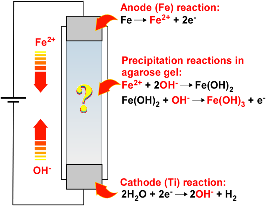
FIGURE 1. Schematic illustration of the reaction–diffusion–reaction (RDR) system, wherein (1) electrochemical reactions to generate reactant ions, (2) diffusion of the reactant ions influenced by an electric field, and (3) reactions of the reactant ions to form precipitates are coupled to generate precipitation patterns of Fe(OH)₃ in agarose hydrogel. The arrows indicate the directions of movement of the reactant ions in the electric field.

The generated Fe²⁺ and OH⁻ ions are transported under the influence of the electric field and thermal diffusion and react with each other to form Fe(OH)₂ precipitates.

$\mathbf{F}{\mathbf{e}}^{\mathbf{2}+}+\mathbf{2}\mathbf{O}{\mathbf{H}}^{‒}\to \mathbf{F}\mathbf{e}{\left(\mathbf{O}\mathbf{H}\right)}_{\mathbf{2}}.(3)$

Due to the solubility-product constant of Eq. 3 being low (4.87 $\times$ 10^–17 [19]), this precipitation reaction occurs easily. Fe(OH)₂ precipitates are relatively unstable in aqueous solution or hydrogel and are rapidly oxidized under the basic condition of pH > 5.

$\mathbf{F}\mathbf{e}{\left(\mathbf{O}\mathbf{H}\right)}_{\mathbf{2}}+\mathbf{O}{\mathbf{H}}^{‒}\to \mathbf{F}\mathbf{e}{\left(\mathbf{O}\mathbf{H}\right)}_{\mathbf{3}}+{\mathbf{e}}^{‒}.(4)$

Because the solubility-product constant of Fe(OH)₃ is considerably low (2.79 $\times$ 10^–39 [19]), the rust-brown Fe(OH)₃ precipitates thus formed are hardly soluble and are expected to form various precipitation patterns at the cathode side (to generate OH⁻ ions) of the agarose hydrogel in the current RDR system. The relative simplicity of the above chemical processes (Eqs 1–4) was initially expected to be convenient in facilitating an understanding of the basic nature of periodic banding in the Cu‒Fe PBA system. However, it generated a completely different type of periodic banding, that is, a new type of non-equilibrium phenomenon described below.

2 Materials and methods

2.1 Materials

The agarose required for electrophoresis (gel strength: 1800–2,300 g/cm³) was purchased from Kanto Chemical (Tokyo, Japan) and used without further purification. All aqueous solutions were prepared using deionized water that had been obtained from purifying tap water using a cartridge water purifier (G-10, Organo, Tokyo, Japan). In addition, Ti (≥99.5%) and Fe (≥99.5%) rods obtained from Nilaco (Tokyo, Japan) were used as the electrodes.

2.2 Sample preparation for observing precipitation patterns

Sample tubes filled with agarose gel (called “gel holders” hereinafter) were prepared as further described. To check reproducibility, at least four gel holders were prepared under the same conditions for each experiment. Appropriate amounts of agarose powder were added to 30 ml deionized water at 25°C to form a 2.0 mass% agarose mixture. The resulting mixture was then stirred vigorously at 98°C for 30 s to produce a uniform agarose sol. Using a Pasteur pipette, the sol was transferred to 4 mm diameter and 45–75 mm long plastic straws, the bottoms of which were plugged with a Ti metal rod (used as the cathode) with a diameter of 4 mm and a length of ∼20 mm. Plastic straws were employed because they are simple to prepare and use, cheap, and support the easy introduction of viscous samples, such as organic sols (or organic colloidal solutions) [20]. The hot sol in the straw was left to cool to 25°C, and a solidified gel was formed, with the solidification time being approximately 10 min. The height of the resulting gel column in the gel holders (L) was 30–60 mm.

A 3 mm diameter and ∼30 mm long Fe metal rod was placed atop the prepared gel column as the anode. Because the Fe anode did not fit tightly inside the straw, it maintained contact with the gel surface even when the electric field had caused the gel column to contract. The cathode and anode were connected to a programmable power supply (PPS303, AS ONE, Osaka, Japan). During the application of constant or cyclic alternating voltages at 25°C (typical current ≈2 μA for 3 V and L = 50 mm), the precipitation patterns formed in the gel were monitored using a digital camera (Tough TG-6, Olympus, Tokyo, Japan).

2.3 Fe Kα intensity distribution measurement

After the voltage application experiments, some gel holders were re-plugged at both ends using styrene-resin stoppers covered with Parafilm for the Fe Kα intensity distribution measurements. These measurements were conducted using a homemade X-ray fluorescence (XRF) setup [21]. Briefly, the excitation source was Cu Kα₁ X-rays from an 18 kW generator (RU-300, Rigaku, Tokyo, Japan) operating at 40 kV and 60 mA, and the beam was focused to within 0.5 mm in the horizontal direction (resultantly, to have a linear shape) by a SiO₂ $\left(10\overline{1}1\right)$ Johansson-type crystal monochromator. The gel holder to be measured was placed perpendicular to the linear X-ray beam on a computer-controlled X-Z stage. XRF signals from the gel holder were detected using a silicon PIN detector (XR-100CR, Amptek, Bedford, MA, United States), and the data were collected for 90 s using a multichannel analyzer (MCA8000A, Amptek). The distribution of the Fe Kα intensity from the gel holder in its axial direction was measured at 25°C by moving the holder in the same direction in 0.5 mm steps. The required collection time to obtain the Fe Kα intensity distribution was approximately 2 h. After subtracting the constant background from the Fe Kα peak, the integrated intensities over 6,214–6,647 eV were used to determine the Fe Kα distribution.

2.4 SEM observation

Subsequent to the Fe Kα distribution measurements, some gel columns were pulled out of the gel holder and cut into ∼1 mm-thick sections. These sections were allowed to dry for a few weeks in the ambient laboratory environment by being stuck on double-sided adhesive carbon tape and mounted on the aluminum stub of a scanning electron microscope (SU8220, Hitachi, Tokyo, Japan). Scanning electron microscopy (SEM) observation was conducted at 10.0 kV at a working distance of 15.2 mm. The XRF intensity map was also obtained using an XRF detector installed in SU8220 (EMAX X-Max^N, Oxford Instruments, Tokyo, Japan) and an analysis software (AZtec Live, Oxford Instruments).

3 Results

3.1 Precipitation patterns under constant voltages

Figure 2A shows the precipitation patterns formed in the gel columns with a length of 50 mm at 25°C under the applied constant voltages of 1, 2, 3, 4, and 5 V for 12 h. In these conditions, a continuous, broad, and diffusive precipitation band (not periodic or discrete) with a rust-brown color characteristic of Fe(OH)₃ was observed. As expected, applying higher voltages significantly lengthened the continuous band and deepened its rust-brown color, suggesting that such higher voltages promoted the generation of reactant ions and, consequently, the precipitation of Fe(OH)₃. Interestingly, the band positions also depended on the applied voltages; higher applied voltages tended to shift the precipitation band to the cathode side.

FIGURE 2

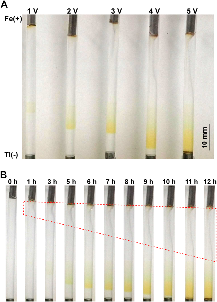
FIGURE 2. (A) Precipitation patterns formed in the gel columns with L = 50 mm at 25°C under the applied constant voltages of 1, 2, 3, 4, and 5 V for 12 h. The charges of the electrodes and a scale bar are provided on the left and right of the image, respectively. (B) Spatiotemporal evolution of the precipitation band formed at 25°C under an applied constant voltage of 5 V. The elapsed time after the application of voltage is indicated at the top of each image. The red broken line encloses the area where the gel column is distorted.

Figure 2B shows the spatiotemporal evolution of the continuous band formed under an applied constant voltage of 5 V for 12 h. After 5 h of the voltage application, a faint, broad rust-brown band formed at the position relatively near the cathode. This band expanded to the cathode side monotonously with time, deepening its rust-brown color without generating periodic bands. After 11 h, the edge of the band reached the cathode surface and its expansion stopped. Such a gradual extension toward the cathode with time was commonly observed under applied constant voltages.

During applications of voltages, the agarose gel gradually distorted with time, mainly at the anode side. Generally, at higher voltages (such as 5 V, Figure 2B) and shorter gel columns (such as 30 mm), such distortion occurred more quickly and largely. For instance, as shown in Figure 2B, the gel column began to shrink near the anode only 1 h after applying 5 V, and approximately half of the gel column was distorted after 12 h. The gel distortion prevented long-time observations even under applied lower voltages. Thus, the observation time in the current experiments, including experiments with cyclic alternating voltages, was limited up to 60 h. It should be noted that gel distortion or shrinkage under electric fields has been observed in various systems [22–24], and related theoretical approaches are being developed [25]; however, the details of the observed distortion are still unclear.

3.2 Periodic band formation under cyclic alternating voltages

3.2.1 Basic features

Figure 3 shows the spatiotemporal evolution of the periodic bands formed at 25°C in the gel columns with L = 50 mm under the applied cyclic alternating voltages of 3 and 1 V for 1 and 4 h, respectively, per cycle, for a total of eight cycles (40 h). As described in Sections 3.2.2‒3.2.4, this experimental condition is the optimal one to less stochastically observe fine periodic bands. Here, the results of four samples that were prepared under the same experimental conditions were presented for comparison because the periodic banding by RDR processes is fundamentally stochastic [16] (hereinafter, the banding images will be shown similarly). Regarding the aforementioned application of cyclic alternating voltages, more reactant ions were produced at 3 V, and the stronger electric field had a greater influence on the ions. In contrast, fewer reactant ions were produced at 1 V, and thermal diffusion exerted a stronger effect on the residual ions. Hereinafter, the higher voltage and its application time shall be represented as E_H and T_H, respectively; the lower voltage and its application time as E_L and T_L, respectively; and the cycle number as N_C. For instance, the values of these parameters in the experiment shown in Figure 3D are E_H = 3 V, E_L = 1 V, T_H = 1 h, T_L = 4 h, and N_C = 8.

FIGURE 3

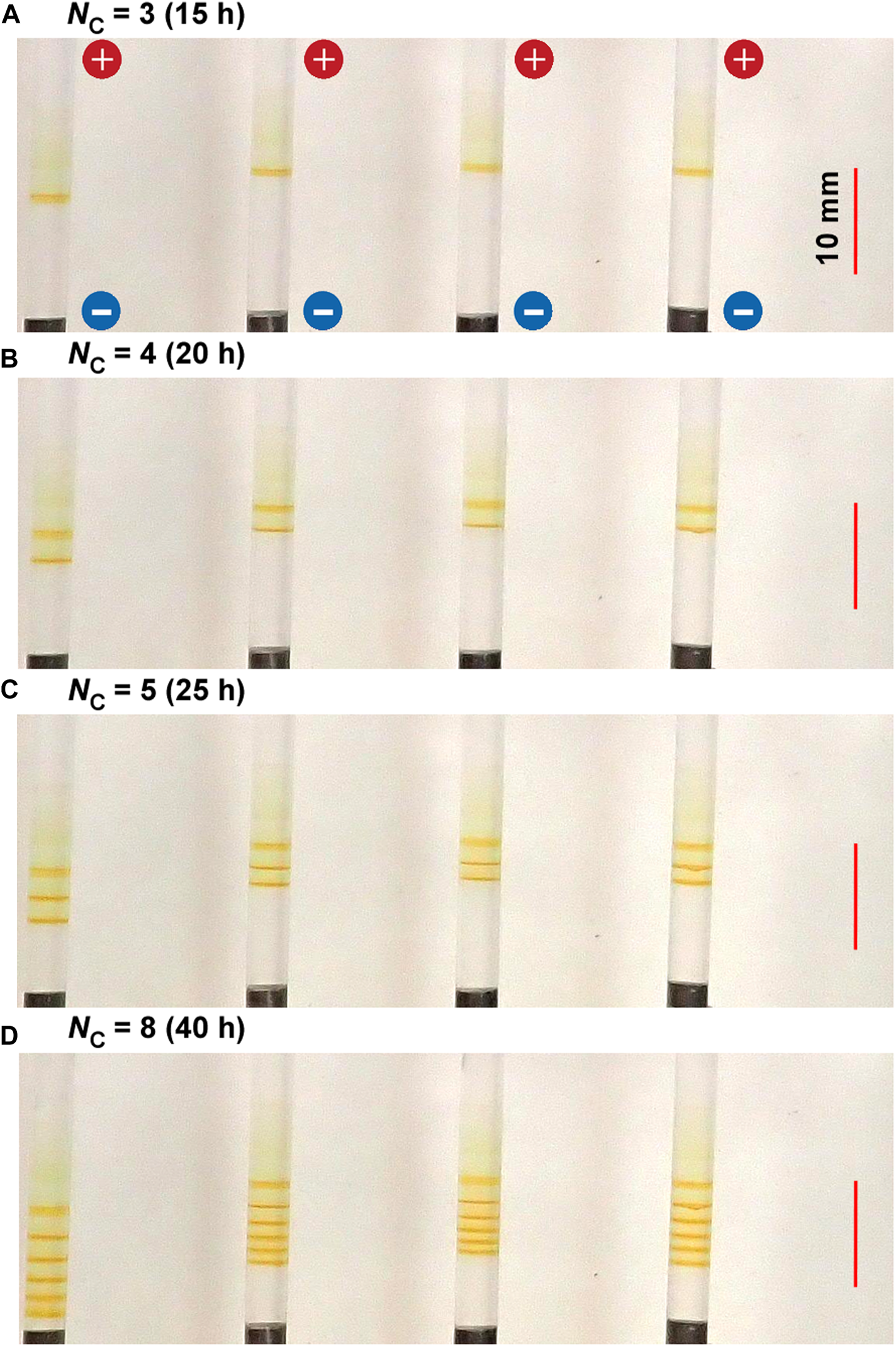
FIGURE 3. Spatiotemporal evolution of typical periodic bands formed in the four gel columns with L = 50 mm at 25°C under the following applied cyclic alternating voltage condition: E_H = 3 V, E_L = 1 V, T_H = 1 h, and T_L = 4 h. The cycle numbers (N_C) are (A) 3 (B) 4 (C) 5, and (D) 8. The elapsed times after the application of voltage are also indicated. The scale bars are provided on the right parts of the images, and the charges of the electrodes are provided in the top image.

In Figure 3, several periodic and discrete (Liesegang-band-like) rust-brown bands that were not observed under constant voltages are clearly observed within a relatively narrow region of approximately 10 mm near the cathode. Interestingly, the periodic banding found in Figure 3 is completely different from that of the previously reported Cu–Fe PBA [16, 17] and Prussian blue (PB) systems [17]. After 10 h of applying the cyclic alternating voltages, a relatively sharp rust-brown band gradually emerged at 12 ± 3 mm from the cathode surface and became distinct up to 15 h (N_C = 3). After 15 h, the second discrete band gradually emerged at the cathode side of the gel holders and became distinct up to 20 h (N_C = 4). After 20 h, the third discrete band was similarly generated at the cathode side. Thus, a discrete band was newly generated at the cathode side with N_C; during the cycle whose cycle number is N_C, N_B = N_C ‒ N_C1 + 1 of the number of periodic bands were observed, where N_C1 is the cycle number for which the first band emerged (e.g., in Figure 3, N_C1 = 3).

Owing to the inherent stochastic property of RDR processes, the periodic patterns of the four samples shown in Figure 3 are not completely similar. Nevertheless, the periodic banding of the current system was much less stochastic than those of the RDR systems of previously reported Cu–Fe PBA [16, 17]. It exhibited the following similar features: a) the periodic bands were formed at the cathode side, maintaining their positions during the observation time; b) the number of periodic bands (N_B) was N_C—N_C1 + 1; and c) the distance between the first and the second emerged band (2.2 ± 0.8 mm) was slightly larger than the distances between the other adjacent bands that seemed to be randomly distributed around an average value with a relatively broad dispersion (1.3 ± 0.8 mm). These features held in additional four replications, each of which comprised four gel columns (thus, total 16 samples) that were prepared under the same experimental conditions.

Notably, the afore-described features were different from those of not only conventional Liesegang banding but also those of the RDR banding of Cu–Fe PBA and PB, possibly reflecting the differences in the mechanisms that form periodic bands. For instance, in typical Liesegang banding systems, the band positions move with time, and the space between adjacent bands increases monotonically, obeying the so-called spacing law X_i+1/X_i = 1 + p, where X_i is the position of the ith band and p > 0 for most systems [3, 4, 6, 10]. In the RDR system of the PB, only a few discrete bands formed at the anode side [17]. In that of the Cu–Fe PBA, periodic bands gradually emerged, shifting in position toward the anode with time (although their positions were near the cathode), and the relation between the band number and cycle number was highly stochastic and unclear [16, 17]. Thus, the periodic banding illustrated in Figure 3 has proven to be unprecedented.

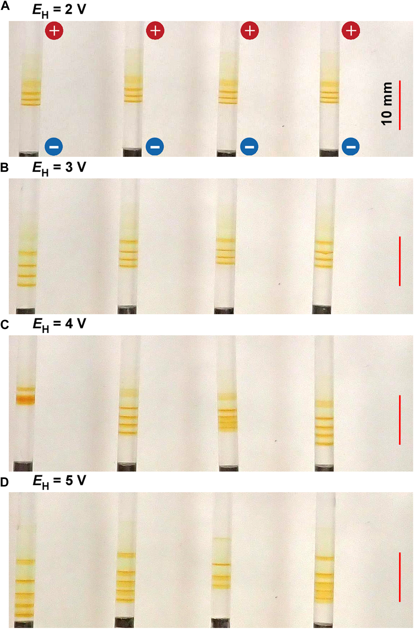
3.2.2 Effect of voltage in the application of cyclic alternating voltages

Figure 4 shows the periodic bands formed in the gel columns with L = 50 mm at 25°C under the applied cyclic alternating voltages of E_L = 1 V, T_H = 1 h, T_L = 4 h, N_C = 6, and the following E_H values A) 2 B) 3 C) 4, and D) 5 V. Figure 4 indicates that the N_B values increase with E_H; N_B = 3 (plus one diffusive band at the top), 4, 4 (plus one diffusive band at the top), and 5 for E_H = 2, 3, 4, and 5 V, respectively. Interestingly, the relation N_B = N_C ‒ N_C1 + 1 held independent of E_H; e.g., the N_C1 values for E_H = 3 V was 3, and that for E_H = 5 V was 2. Here, the diffusive band at the top observed for E_H = 2 V and 4 V was not considered as the periodic band. The treatment of the diffusive bands shall be discussed in Section 4.1.

FIGURE 4

FIGURE 4. Typical periodic bands formed in the four gel columns with L = 50 mm at 25°C under the E_H values (A) 2 (B) 3 (C) 4, and (D) 5 V. Here, E_L = 1 V, T_H = 1 h, T_L = 4 h, and N_C = 6 are kept constant. The scale bars are provided on the right parts of the images, and the charges of the electrodes are provided in the top image.

The increase in E_H also resulted in a slight but noticeable increase in the band width and the stochasticity in the positions of the periodic bands (e.g., compare the images for E_H = 2 and 5 V). As a result, under higher E_H conditions, the discrete bands occasionally overlapped one another, apparently reducing the N_B values (see the leftmost sample for E_H = 4 V and the second sample from the right for E_H = 5 V in Figure 4).

The large band number and wide bandwidth suggested that large amounts of Fe(OH)₃ had been precipitated in the system. Meanwhile, the high stochasticity in the band position implied the high possibility of the precipitation reactions, namely Eqs 3, 4, occurring all over the system. Thus, the above observations can be directly attributed to the increase in reactant ions generated by applying higher E_H. Higher E_H values are also expected to influence the transport properties of the generated ions more strongly, contributing to the above observations. However, this effect has not been well examined yet.

In contrast, with the decrease in E_H, the discrete bands decreased in number and decolored, although the bandwidth and position stochasticity decreased. Resultantly, the periodic banding was most clearly observed around the intermediate E_H value (3 V).

Figure 5 shows the typical periodic bands formed in the gel columns with L = 50 mm at 25°C under the applied cyclic alternating voltages of E_H = 3 V, T_H = 1 h, T_L = 4 h, N_C = 6, and the following E_L values A) 0.1 B) 1, and C) 2 V. The E_L values also considerably influenced the periodic banding. In the condition wherein almost no voltage had been applied (E_L = 0.1 V, Figure 5A), although the first band (the one closest to the anode) was clearly noticeable, the following bands were not clearly distinguishable because the spaces between the bands were considerably narrow. This finding suggested that the diffusion process without an electric field is ineffective in separating the discrete precipitation bands and that E_L ≥ 1 V applications are required for clearly separating the bands as shown in Figure 5B (E_L = 1 V).

FIGURE 5

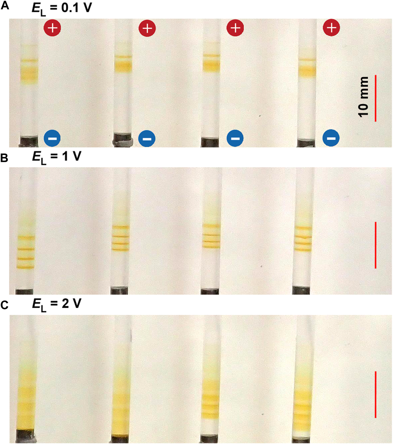
FIGURE 5. Typical periodic bands formed in the four gel columns with L = 50 mm at 25°C under the E_L values (A) 0.1 (B) 1, and (C) 2 V. Here, E_H = 3 V, T_H = 1 h, T_L = 4 h, and N_C = 6 are kept constant. The scale bars are provided on the right parts of the images, and the charges of the electrodes are provided in the top image.

Meanwhile, under a higher E_L condition (E_L = 2 V), five periodic bands that followed the relation N_B = N_C ‒ N_C1 + 1 = 6–2 + 1 = 5 and shifted their positions to the cathode side were barely noticeable, largely increasing their bandwidths. Notably, rust-brown precipitates considerably emerged at these spaces, occasionally forming an almost-continuous band (e.g., see the left two samples in Figure 5C). As a result, the periodic banding was most clearly observed around the intermediate E_L value (1 V).

3.2.3 Effect of period in the application of cyclic alternating voltages

Figure 6 shows the typical periodic bands formed in the gel columns with L = 50 mm at 25°C under the applied cyclic alternating voltages of E_H = 3 V, E_L = 1 V, T_L = 4 h, N_C = 8, and the following T_H values A) 0.5 B) 1, and C) 2 h. The N_B values increased with T_L; N_B = 5 (plus one diffusive band at the top), 6, and 6 (plus one diffusive band at the top) for T_H = 0.5, 1, and 2 h, respectively. The relation N_B = N_C ‒ N_C1 + 1 held independent of T_H. The increase in T_H also resulted in an increase in the spaces between the adjacent bands. Meanwhile, because the broadened spaces were occasionally painted out at the longer T_H (see the rightmost sample in Figure 6C), the periodic banding at the longer T_H (2 h) was not necessarily clearer than that at the intermediate T_H (1 h). Additionally, as exhibited in the left two samples of Figures 6A,C larger gel distortion extending to the vicinity of the cathode often occurred at larger T_H conditions. Resultantly, the periodic banding was most clearly observed around the intermediate T_H value (1 h).

FIGURE 6

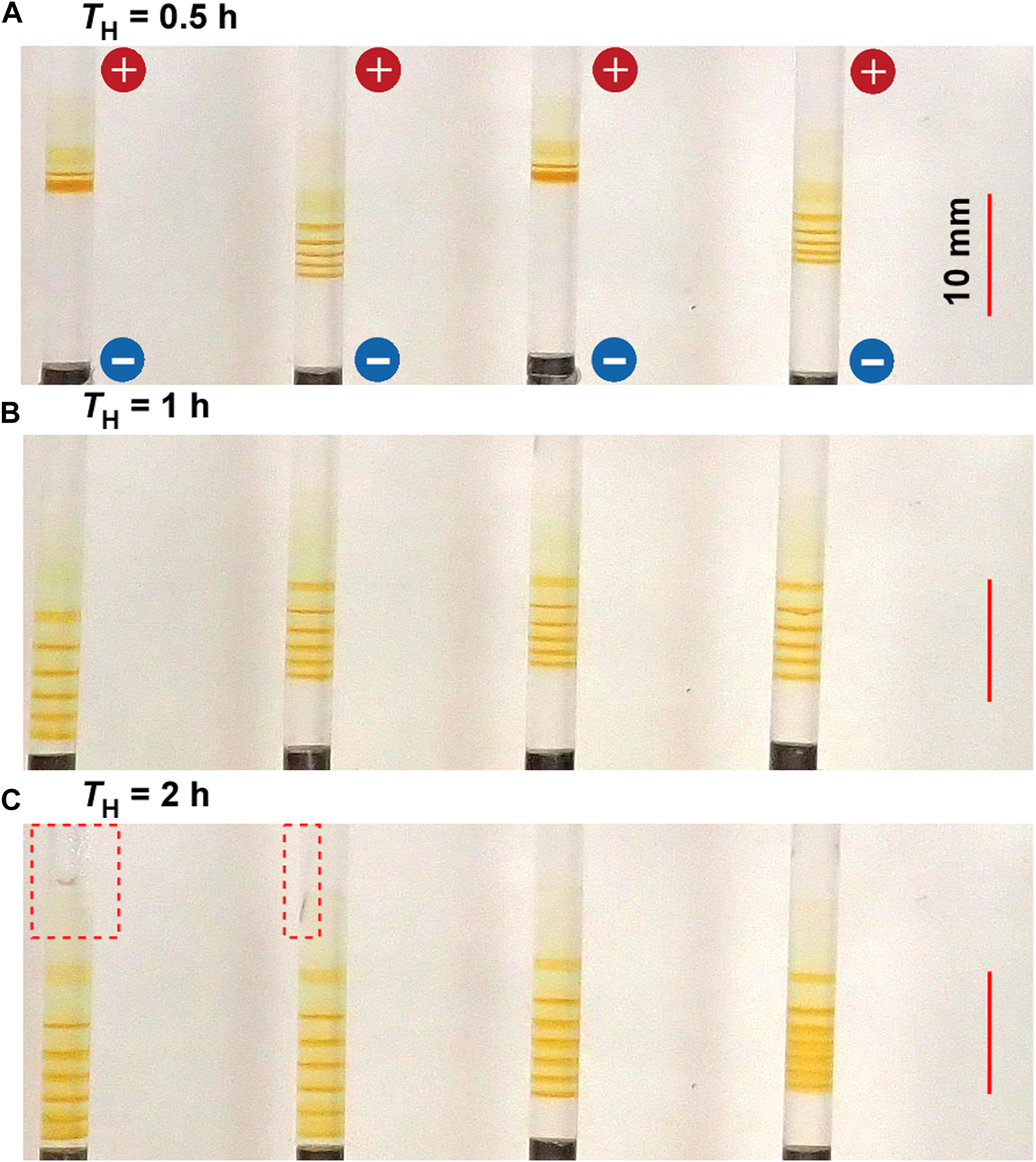
FIGURE 6. Typical periodic bands formed in the four gel columns with L = 50 mm at 25°C under the T_H values (A) 0.5 (B) 1, and (C) 2 h. Here, E_H = 3 V, E_L = 1 V, T_L = 4 h, and N_C = 8 are kept constant. The scale bars are provided on the right parts of the images, and the charges of the electrodes are provided in the top image. The red broken squares enclose the area where the gel columns are distorted.

Figure 7 shows the typical periodic bands formed in the gel columns with L = 50 mm at 25°C under the applied cyclic alternating voltages of E_H = 3 V, E_L = 1 V, T_H = 1 h, N_C = 8, and the following T_L values A) 2 B) 4, and C) 6 h. Interestingly, the results shown in Figure 7 are similar to those in Figure 6. For instance, a) the N_B values increased with T_L; N_B = 5 (plus one diffusive band at the top), 6, and 6 (plus one diffusive band at the top) for T_L = 2, 4, and 6 h, respectively, adhering to the relation N_B = N_C ‒ N_C1 + 1; and b) the increase in T_L tended to broaden the spaces between the adjacent bands. Obviously, the T_H and T_L dependences were not considerably similar. For instance, the longer T_L also brought about stochasticity in the positions of the periodic bands, and consequently, the periodic bands occasionally overlapped to generate a thick, almost-continuous single band (e.g., see the leftmost sample in Figure 7C). Consequently, the periodic banding was most clearly observed around the intermediate T_L value (4 h). In contrast, the painting-out effects, observed at the longer T_H conditions (Figure 6), were unclear at longer T_L conditions. Nevertheless, overall, the effects of increasing the T_H and T_L values were similar. Noteworthily, they were also similar to the effects of increasing the E_H and E_L values (see Figures 4, 5). The similarity of the influences on N_B was evident and particularly interesting, and this shall be explored in further detail in Section 4.1.

FIGURE 7

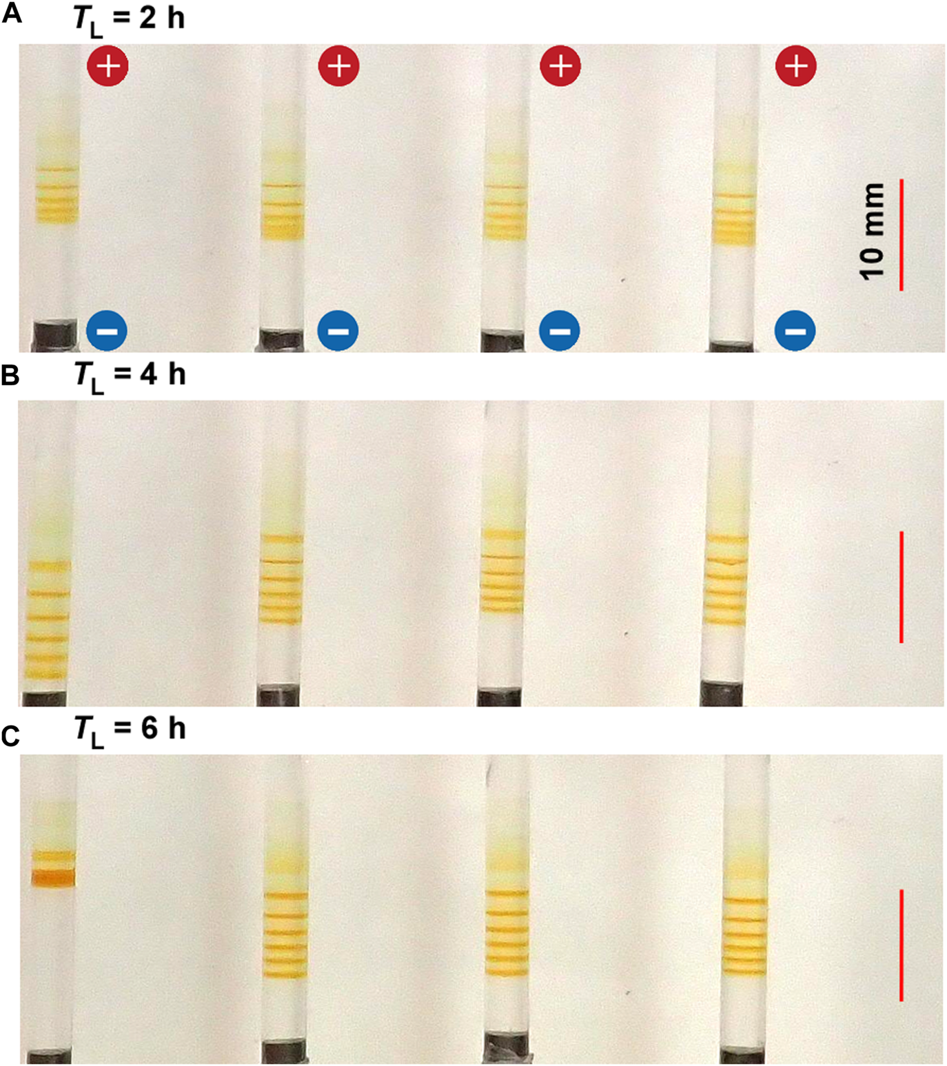
FIGURE 7. Typical periodic bands formed in the four gel columns with L = 50 mm at 25°C under the T_L values (A) 2 (B) 4, and (C) 6 h. Here, E_H = 3 V, E_L = 1 V, T_H = 1 h, and N_C = 8 are kept constant. The scale bars are provided on the right parts of the images, and the charges of the electrodes are provided in the top image.

3.2.4 Effect of gel length

Figure 8 shows the typical periodic bands formed in the gel columns for various L values at 25°C under the applied cyclic alternating voltages (E_H = 4 V, E_L = 1 V, T_H = 1 h, T_L = 4 h, and N_C = 5) A) L = 30 B) 40 C) 50, and D) 60 mm. Here, the E_H value of 3 V, employed for the experiments whose results are shown in Figures 3, 5‒7, was not used. Instead, the E_H value of 4 V was used because the L-dependence of the N_B values for E_H = 4 V could be less ambiguously examined than that for E_H = 3 V (see Section 4.1).

FIGURE 8

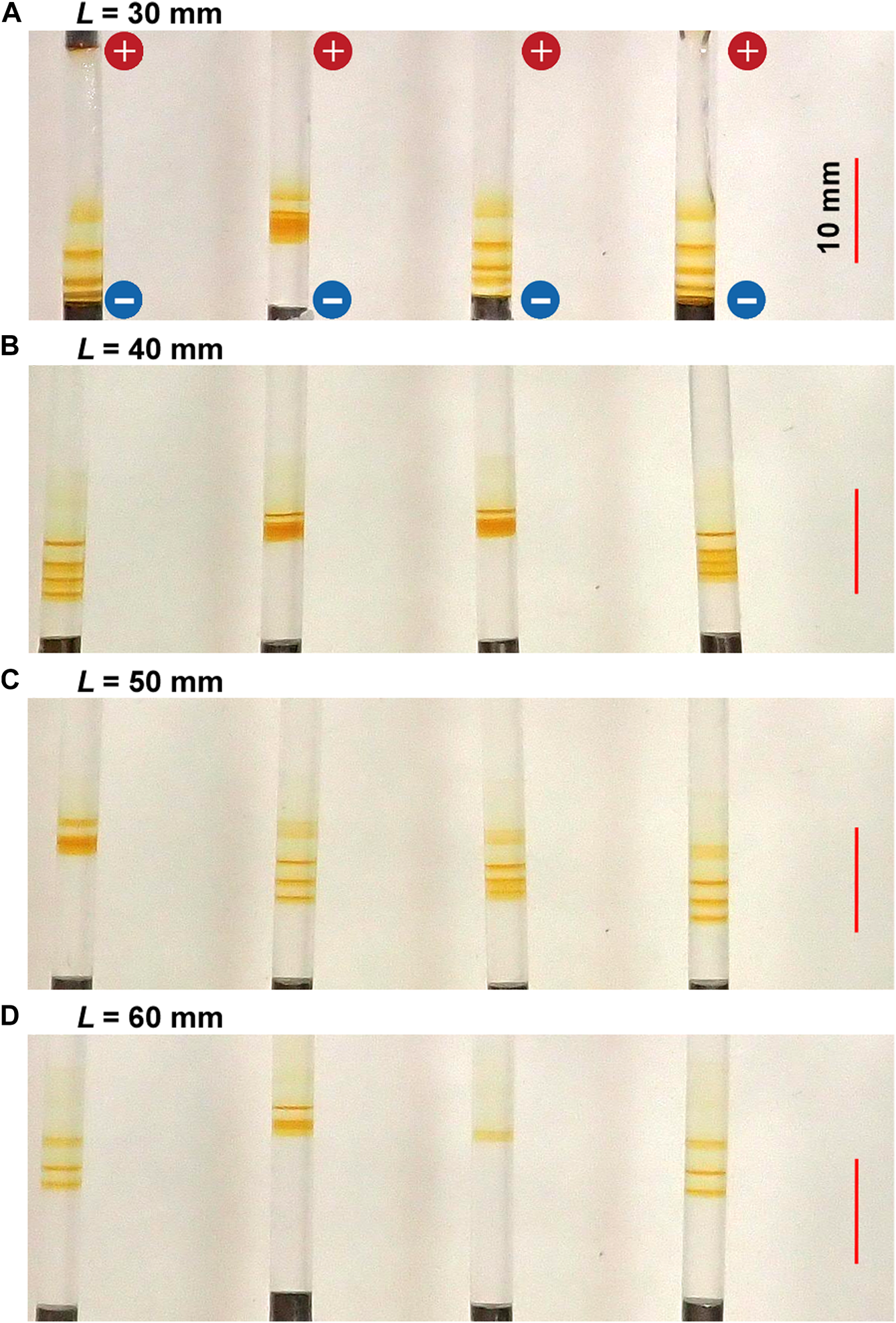
FIGURE 8. Typical periodic bands formed in the four gel columns with various lengths (L) at 25°C under the applied cyclic alternating voltages (E_H = 4 V, E_L = 1 V, T_H = 1 h, T_L = 4 h, and N_C = 5): (A) L = 30 (B) 40 (C) 50, and (D) 60 mm. The scale bars are provided on the right parts of the images, and the charges of the electrodes are provided in the top image.

The length of the gel columns also strongly influenced the periodic banding. In shorter gel columns, such as those with L = 30 mm, thick periodic bands formed relatively quickly. For instance, one discrete band was generated after 5 h (N_C = 2). Meanwhile, the positions of the periodic bands were significantly stochastic, which occasionally resulted in the overlapping of the discrete bands to generate a seemingly single and relatively broad band (see the second sample from the left in Figure 8A). Considering such overlaps, the relation N_B = N_C ‒ N_C1 + 1 still held independent of L, strongly suggesting the importance of this relation in the current RDR system. However, when the positions of the latest generated band were close to the surface of the cathode, no more periodic bands emerged, disobeying this relation. For instance, for L = 30 mm, three periodic bands (plus one diffusive band at the top) were observed for N_C = 4 (not shown here), obeying this relation as follows: N_C ‒ N_C1 + 1 = 4–2 + 1 = 3. However, the fourth periodic band was not generated for N_C = 5 (Figure 8A) because the positions of the third periodic band were too close to the cathode surface.

In contrast, in longer gel columns, such as those with L = 60 mm (Figure 8D), the number of periodic bands was minimal and discoloring was observed. Similar trends were observed independent of E_H, E_L, T_H, and T_L. Resultantly, the periodic banding was most clearly observed around the intermediate L value (50 mm).

3.3 Fe Kα intensity distribution

Figure 9 shows the Fe Kα intensity distribution of the gel column having periodic bands formed at 25°C under the applied cyclic alternating voltages: E_H = 3 V, E_L = 1 V, T_H = 1 h, T_L = 4 h, and N_C = 8; the horizontal axis indicates the distance from the cathode surface (X), where X > 0 is on the anode side, and the vertical axis is the relative Fe Kα intensity. As already shown in previous studies [26, 27], the Fe Kα distributions of hydrogels having Fe-related precipitates provide a good estimate of the Fe elemental distributions.

FIGURE 9

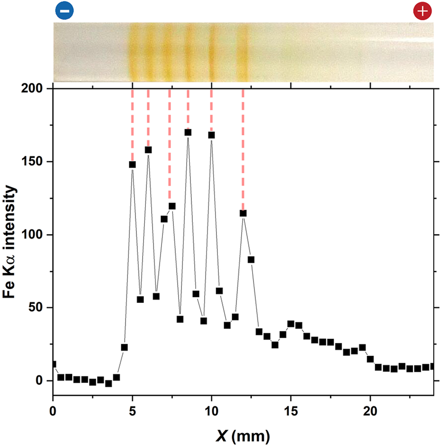
FIGURE 9. Fe Kα intensity distribution of the periodic bands formed in the gel column of L = 50 mm at 25°C under the following applied cyclic alternating voltages: E_H = 3 V, E_L = 1 V, T_H = 1 h, T_L = 4 h, and N_C = 8. An image of the gel column is displayed at the top to facilitate comparison with the periodic bands. The charges of the electrodes, which have been used for preparation, are provided at the top of the image. The vertical dashed lines serve as guides.

In Figure 9, six sharp Fe Kα distribution peaks can be observed, with their peak positions agreeing well with the positions of the periodic bands. This result strongly supported the assumption that rust-brown periodic bands comprised considerable amounts of Fe(OH)₃. Interestingly, the Fe Kα distribution was not observed near the cathode (X < 4 mm). This finding suggested that the Fe ions at the cathode side of the discrete band that emerged in each cycle (in Figure 9, the leftmost band at X = 5 mm, which emerged at N_C = 8), if any, were fully precipitated as Fe(OH)₃, promoting the growth of the band.

3.4 SEM observation

Figure 10 shows a typical SEM image of the rust-brown band formed in the gel columns with L = 50 mm at 25°C under the applied cyclic alternating voltages: E_H = 3 V, E_L = 1 V, T_H = 1 h, T_L = 4 h, and N_C = 8. The Fe Lα intensity map shown as pink dots in Figure 10, was overlapped for comparison. At the bottom of the SEM image, an XRF spectrum is provided. Here, all the measured XRF intensities (including Fe Lα intensities) have been added over the area of the SEM image. The estimated weight % values of the detected elements are tabulated at the right side of the spectrum.

FIGURE 10

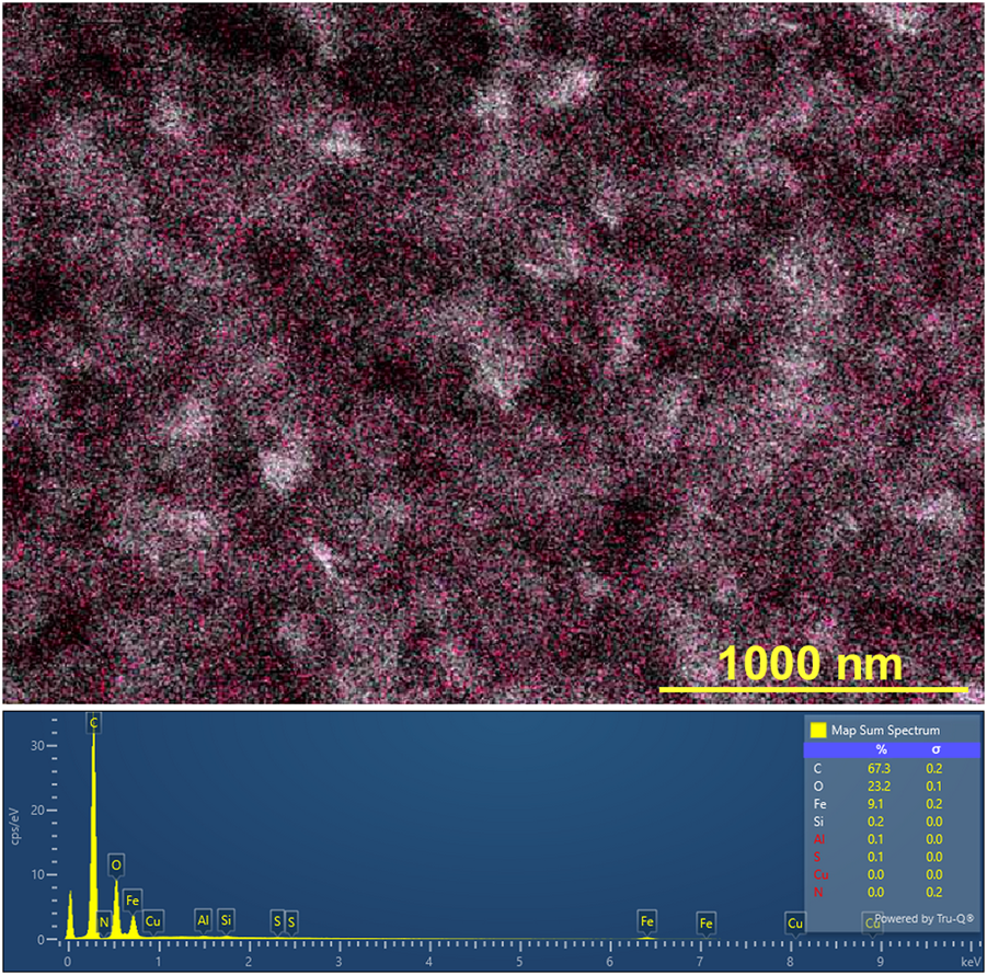
FIGURE 10. (Top) Scanning electron microscope (SEM) image (× 40,000) of the rust-brown band formed in the gel columns with L = 50 mm at 25°C under the following applied cyclic alternating voltages: E_H = 3 V, E_L = 1 V, T_H = 1 h, T_L = 4 h, and N_C = 8. Here, the Fe Lα intensity map (the observed positions are shown as pink dots) is overlapped, and a scale bar is provided on the lower right part of the image. (Bottom) X-ray fluorescence (XRF) spectrum, where all the measured XRF intensities have been added over the area of the above SEM image. The estimated weight % values of the detected elements are tabulated on the right side of this spectrum.

Figure 10 indicates that several structures found in the SEM image mainly consist of C, O, and Fe atoms. Furthermore, it establishes that Fe atoms are uniformly distributed over the structures. The presence of the C and O atoms can be attributed to the agarose gel, while the Fe atoms come from the Fe compound(s), which is expected to be Fe(OH)₃ according to Eq. 4, generated by the RDR processes. The uniform distribution of Fe atoms, commonly observed for all the rust-brown bands obtained, strongly suggested that the precipitates formed in the current system essentially comprised not crystalline but gelatinous Fe(OH)₃. This finding is consistent with the well-known fact that Fe(OH)₃ is generally present as colloidal gel in aqueous conditions [28].

4 Discussion

4.1 Relationship between N_B and E_H, E_L, T_H, T_L, and L

Sections 3.2.2‒3.2.4 demonstrated that the patterns of the periodic bands change largely by varying each parameter E_H, E_L, T_H, T_L, and L. The banding patterns also changed by simultaneously varying these parameters. Nevertheless, the basic features a) and b) described in Section 3.2.1 (that is, the immobile periodic bands at the cathode side, of which N_B values are basically given by N_C ‒ N_C1 + 1) generally held. The N_B values in the periodic bands obtained for arbitrary sets of E_H, E_L, T_H, T_L, L, and N_C can be estimated in the manner described below. Here, note that the N_B values can be decreased by the overlapping of the discrete bands owing to the inherent stochasticity of the band positions, as shown in Figure 4C; Figure 6A; Figure 7C; Figure 8. The decrease can also be achieved through the generation of the band close to the cathode surface, as suggested by Figure 8A. However, it should be noted that these effects were not considered in the following N_B estimation.

Figure 11 illustrates the linear correlation between A) N_C1 and E_H B) N_C1 and E_L C) N_C1 and T_H D) N_C1 and T_L, and E) N_C1 and L. Here, the results shown in Figures 3‒8 are considered. In this analysis, we considered the diffusive band that occasionally emerges in the N_C1 cycle and has more than 5-times broader width than the other periodic bands (see Figure 4A; Figure 4C; Figure 6A; Figure 6C; Figure 7A; and Figure 7C) as the “0.5 band”. Hence, some N_B and N_C1 values are half-integer values. Such half-integer N_B values, e.g., d.5, denote that there were d discrete bands plus one diffusive band (0.5) in that gel column. The half-integer N_C1 values, e.g., d’.5, denote that a diffusive band emerged in the d’ cycle, and subsequently, the first discrete band emerged in the d’+1 cycle.

FIGURE 11

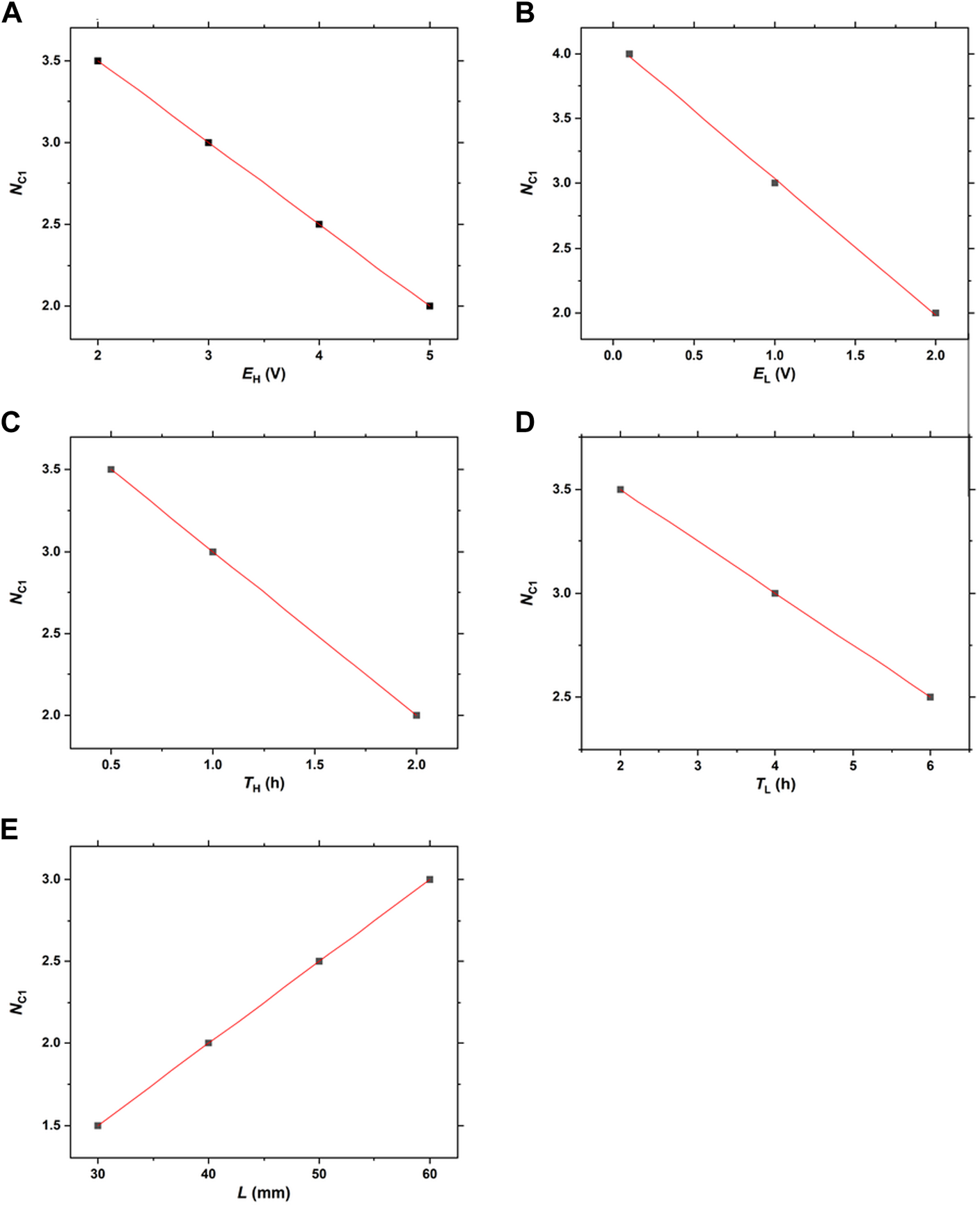
FIGURE 11. Linear correlations between (A) N_C1 and E_H (B) N_C1 and E_L (C) N_C1 and T_H (D) N_C1 and T_L, and (E) N_C1 and L.

Figure 11 indicates that the N_C1 values have good linear correlations with E_H, E_L, T_H, T_L, and L. Based on the results presented in Figure 11, the following linear relationships can be deduced:

${\mathit{N}}_{\mathbf{C}\mathbf{1}}=\mathbf{4.5}–\mathbf{0.5}{\mathit{E}}_{\mathbf{H}},(5)$

${\mathit{N}}_{\mathbf{C}\mathbf{1}}=\mathbf{4}–{\mathit{E}}_{\mathbf{L}},(6)$

${\mathit{N}}_{\mathbf{C}\mathbf{1}}=\mathbf{4}–{\mathit{T}}_{\mathbf{H}},(7)$

${\mathit{N}}_{\mathbf{C}\mathbf{1}}=\mathbf{4}–\mathbf{0.25}{\mathit{T}}_{\mathbf{L}},(8)$

${\mathit{N}}_{\mathbf{C}\mathbf{1}}=\mathbf{0.05}\mathit{L}.(9)$

Here, N_C1 values need to be positive, with these equations suggesting the upper limits of E_H, E_L, T_H, and T_L: E_H < 9 V, E_L < 4 V, T_H < 4 h, and T_L < 16 h. Furthermore, the slope values of these equations quantitatively suggest the extent of the influences of the E_H, E_L, T_H, and T_L values on the N_C1 values, and consequently, the N_B values: E_L = T_H (1) > E_H (0.5) > T_L (0.25). The relatively strong effects of E_L and T_H on N_B, as implied in Figures 5, 6, were quantitatively confirmed here.

By summarizing Eqs. 5‒9, Eq. 10 can be obtained as follows:

${\mathit{N}}_{\mathbf{C}\mathbf{1}}=\left(\mathbf{7.5}–\mathbf{0.5}{\mathit{E}}_{\mathbf{H}}–{\mathit{E}}_{\mathbf{L}}–{\mathit{T}}_{\mathbf{H}}–\mathbf{0.25}{\mathit{T}}_{\mathbf{L}}\right)\times \mathbf{0.02}\mathit{L}.(10)$

Eq. 10 restricts the upper limits of E_H, E_L, T_H, and T_L more severely than Eqs. 5‒9 do. For instance, for E_H = 4 V, E_L = 2 V, and T_L = 6 h, T_H needs to be less than 2 h. By combining the relation N_B = N_C ‒ N_C1 + 1 with Eq. 10, Eq. 11 can be derived:

${\mathit{N}}_{\mathbf{B}}={\mathit{N}}_{\mathbf{C}}–\left(\mathbf{7.5}–\mathbf{0.5}{\mathit{E}}_{\mathbf{H}}–{\mathit{E}}_{\mathbf{L}}–{\mathit{T}}_{\mathbf{H}}–\mathbf{0.25}{\mathit{T}}_{\mathbf{L}}\right)\times \mathbf{0.02}\mathit{L}+\mathbf{1}.(11)$

By Eq. 11, the N_B values for an arbitrary set of E_H, E_L, T_H, T_L, L, and N_C can be estimated within the limit imposed by Eq. 10. Here, the minus N_B values in Eq. 11 denote that no precipitation band emerges in the corresponding N_C cycle. For instance, regarding the condition of E_H = 3 V, E_L = 1 V, T_H = 1 h, T_L = 4 h, L = 50 mm, and N_C = 8, the corresponding N_C1 and N_B values are estimated to be three and six by Eqs 10, 11, respectively. These N_C1 and N_B values agree with the results shown in Figures 3A, D.

In the current RDR system, the band that emerges in the N_C1 cycle, called “the first-observed band” hereinafter, showed particularly diverse features, depending on the values of E_H, E_L, T_H, T_L, and L. More specifically, the first-observed band was qualitatively classified as either periodic, diffusive, or indistinguishable (as periodic or diffusive), or was nearly non-existent due to large thinness. This diversity of the first-observed band was included into the current N_B estimation as follows. In examining the linear correlations in Figure 11, the number of the first-observed band (N_B1) was set for 0, 0.5, and 1, respectively, when the band does not exist, is diffusive, or is periodic. By extension, the N_B1 values for the extremely faint first-observed band are considered as 0 (none) < N_B1 < 0.5 (diffusive). Similarly, the N_B1 values for the first-observed band difficult to be distinguished as either diffusive or periodic are considered as 0.5 (diffusive) < N_B1 < 1 (periodic). Thus, the diverse feature of the first-observed band is reflected as decimal values of N_B in Eq. 11. Based on this consideration, the decimal (non-half-integer) N_B value (d₁. d₂) can be interpreted as follows. The decimal N_B value with d₂ < 5 denotes that, there are d₁ periodic bands and possibly one faint band; the decimal N_B value with d₂ > 5 denotes that, there are d₁ periodic bands and one band difficult to be distinguished as either diffusive or periodic. Thus, the N_B values given by Eq. 11 can suggest not only the number of periodic bands but also the qualitative features of the first-observed band. Note that the suggestion by N_B for the features of the first-observed bands is not quantitative because a) the above discussion concerning N_B1 is qualitative and b) the criterion employed for the diffused band (more than 5-times broader bandwidths than those of other periodic bands) is temporary and lacks physical basis.

For instance, regarding the condition of E_H = 3 V, E_L = 1 V, T_H = 1 h, T_L = 4 h, and N_C = 5, the N_B values for L = 30, 40, 50, and 60 mm are estimated to be 4.2, 3.6, 3, and 2.4, respectively. Several values are decimal, suggesting that the features of some first-observed bands are undesirable in determining N_B and N_C1 values unambiguously. Although not presented here, our observation overall agreed with this suggestion. In contrast, regarding the condition of E_H = 4 V, E_L = 1 V, T_H = 1 h, T_L = 4 h, and N_C = 5, it was relatively easy to count the periodic bands, because the features of the first-observed bands were relatively manageable (Figure 8), as suggested by the integer/half-integer N_B values estimated by Eq. 11: 4.5, 4, 3.5, and 3 for L = 30, 40, 50, and 60 mm, respectively. Thus, the condition of E_H = 4 V was selected for examining the L-dependence of the periodic bands in Section 3.2.4.

As suggested by Eq. 11, the decimal values of E_H, E_L, T_H, T_L, and L generally resulted in the first-observed bands with features expressed by the decimal N_B values. For instance, regarding the condition of E_H = 3.2 V, E_L = 1.6 V, T_H = 1 h, T_L = 4 h, and N_C = 5, the first-observed band was difficult to be distinguished as either diffusive or periodic, as suggested by the decimal N_B value (3.7) estimated by Eq. 11. If the uncertainty of the N_B values within ±1 (owing to the features of the first-observed band) is less emphasized, there is no particular reason for ignoring the decimal values of E_H, E_L, T_H, T_L, and L in observation of the banding.

4.2 Future issues

The simple RDR system proposed in this study can produce Liesegang-band-like, periodic precipitation bands under applied cyclic alternating voltages. Temporal oscillations, such as cyclic alternating voltages, occasionally mediate the formation of spatially extended structures such as periodic bands [10]. Therefore, the periodic banding shown in Figures 3‒8 might not seem a novel finding at first sight. However, this type of periodic banding has not been reported so far, and its formation mechanism is completely unknown. Many theoretical and experimental challenges regarding this type of banding remain across several scientific fields.

Currently, the reason why using cyclic alternating voltages can generate periodic bands that obey the relation N_B = N_C ‒ N_C1 + 1 is unknown. Investigating this question requires a deep understanding of the influences of thermal diffusion and electric field on the movement of the generated ions in agarose gel under applied cyclic alternating voltages. No mathematical model regarding this is currently available (such lack of theoretical model(s) has been occasionally part of a first experimental investigation of pattern formation by precipitation reactions [2, 6]). However, as a starting point toward a theoretical framework, a study on the electric-field effect on Liesegang banding [29] may be useful. Based on such theoretical efforts, it should be clarified what factors determine the optimal experimental condition to observe fine periodic bands less stochastically: E_H = 3 V, E_L = 1 V, T_H = 1 h, T_L = 4 h, and L = 50 mm.

Figure 9 shows the Fe Kα intensity distribution of the gel column having periodic bands after forming under an application of the cyclic alternating voltages. If in situ time-resolved Fe Kα measurements such as those previously conducted for a Liesegang banding system [27] could be conducted, the temporal variation of the Fe amounts in the precipitates under each voltage application condition will be deduced. Such information will be effective for examining the quantitative precipitation kinetics under both constant and cyclic alternating voltages, which may promote the theoretical efforts discussed above. Unfortunately, the timescale of the current T_H + T_L (typically 5 h) is comparable with that of the XRF measurements in our laboratory (∼2 h required). In this situation, the measurement time of XRF will strongly affect the periodic banding. This difficulty can be addressed by using synchrotron radiation (SR) because the timescale of the XRF measurements using SR is approximately 10 min, thereby resulting in plans toward conducting future SR experiments.

Time-resolved measurements of UV-visible (UV-Vis) absorption spectra are also interesting because the spectra can distinguish between Fe(II) and Fe(III) compounds. By combining the Fe Kα distributions, the emergence timing and temporal growth of the newly formed precipitation band will be more quantitatively studied, making a connection with the band characters, such as diffused, discrete, and intermediate. To obtain UV-Vis distributions in the gel column, a line-focusing UV-Vis source and a customized setup for moving the gel holder are required. Such experimental setup is currently in the design process.

The gel distortion at the anode side as shown in Figures 2, 6C should be further investigated to clarify its influence on periodic banding. Detailed electrochemical measurements at the anode side may help solve this issue. To conduct such electrochemical experiments, we are currently embedding a picoammeter and a reference electrode into the RDR setups. Further, the importance of pH for hydrogel distortion has been suggested in some studies [30, 31], and hence, in situ pH measurements over the gel column during the application of cyclic alternating voltages are intriguing. Hence, some pH probes installable into the current RDR system are being considered.

The generated precipitates did not consist of crystallites (such as Cu‒Fe PBA systems [16]) but gel, as suggested by Figure 10. Determining whether the observed periodic banding depends on the gelatinous nature of the reaction products is interesting. For this purpose, the generated rust-brown precipitates (Fe(OH)₃ gel) need to be more comprehensively characterized. We are currently planning to investigate the local structure around the Fe atoms in the gelatinous precipitates by measuring X-ray absorption fine structure (XAFS) at SR facilities [26]. Furthermore, the general importance of dissipation for self-assembled structures has recently been demonstrated [9]. Hence, concurrently with XAFS measurements, the energy and matter dissipation inherent to gel formation should be theoretically examined for the current RDR system.

A previous study [17] indicated that the substitution of electrodes in RDR system causes drastic changes in precipitation patterns. By substituting the Co, Ni, and Zn anodes for an Fe anode, the RDR patterning of Co(OH)₂, Ni(OH)₂, and Zn(OH)₂ can be examined using the current setup. The solubility-product constants of Co(OH)₂, Ni(OH)₂, and Zn(OH)₂ with values 5.92 $\times$ 10^–15, 5.48 $\times$ 10^–16, and 3 $\times$ 10^–17, respectively, are comparable with that of Fe(OH)₂ (4.87 $\times$ 10^–17) and considerably higher than that of Fe(OH)₃ (2.79 $\times$ 10^–39) [19]. Hence, such experiments may be helpful in elucidating the effects of low solubility of Fe(OH)₃ precipitates on the periodic banding under the RDR processes; preliminarily experiments are in progress.

5 Conclusion

In a simple RDR system, Liesegang-band-like, periodic precipitation bands were generated under applied cyclic alternating voltages. The precipitation bands contained significant amounts of Fe atoms, which were uniformly distributed in the agarose gel, strongly supporting the formation of Fe(OH)₃ gel in the bands. In this RDR system, the number of the periodic bands (N_B) could be controlled via the empirical relation, N_B = N_C ‒ N_C1 + 1, and the optimal experimental condition for clearly observing periodic bands less stochastically was E_H = 3 V, E_L = 1 V, T_H = 1 h, T_L = 4 h, and L = 50 mm. This novel and interesting periodic banding system, as well as other RDR systems [16, 17], is expected to broaden the research field of non-equilibrium physics. Hence, these RDR systems warrant further investigation.

Data availability statement

The original contributions presented in the study are included in the article/supplementary material, further inquiries can be directed to the corresponding author.

Author contributions

HH conceived the concept, performed the experiments, analyzed the results, wrote the manuscript, and prepared the figures.

Funding

This research was funded by JSPS KAKENHI (grant number JP19K05409).

Acknowledgments

The author is grateful to T. Takagi of the Laboratory of Electron Microscopy, Japan Women’s University for her SEM operation.

Conflict of interest

The author declares that the research was conducted in the absence of any commercial or financial relationships that could be construed as a potential conflict of interest.

Publisher’s note

All claims expressed in this article are solely those of the authors and do not necessarily represent those of their affiliated organizations, or those of the publisher, the editors and the reviewers. Any product that may be evaluated in this article, or claim that may be made by its manufacturer, is not guaranteed or endorsed by the publisher.

References

1. Karam T, El-Rassy H, Nasreddine V, Zaknoun F, El-Joubeily S, Eddin AZ, et al. Pattern formation dynamics in diverse physico-chemical systems. Chaotic Model Simul (2013) 3:451–61.

Google Scholar

2. Nakouzi E, Steinbock O. Self-organization in precipitation reactions far from the equilibrium. Sci Adv (2016) 2:e1601144. doi:10.1126/sciadv.1601144

PubMed Abstract | CrossRef Full Text | Google Scholar

3. Nabika H, Itatani M, Lagzi I. Pattern formation in precipitation reactions: The Liesegang phenomenon. Langmuir (2020) 36:481–97. doi:10.1021/acs.langmuir/9b03018

PubMed Abstract | CrossRef Full Text | Google Scholar

4. Nabika H. Liesegang phenomena: Spontaneous pattern formation engineered by chemical reactions. Curr Phys Chem (2015) 5:5–20. doi:10.2174/187794680501150908110839

CrossRef Full Text | Google Scholar

5. Sadek S, Sultan R. Liesegang patterns in nature: A diverse scenery across the sciences. In: I Lagzi, editor. Precipitation patterns in reaction–diffusion systems. India: KeralaResearch Signpost (2010). p. 1–43.

Google Scholar

6. Henisch HK. Crystals in gels and Liesegang rings. Cambridge, UK: Cambridge University Press (1988). p. 116–75.

Google Scholar

7. Liesegang RE. Ueber einige eigenschaften von gallerten. Naturwi Wochenschr (1896) 11:353–62. doi:10.1007/BF01830142

CrossRef Full Text | Google Scholar

8. Arango-Restrepo A, Barragán D, Rubi JM. Self-assembling outside equilibrium: Emergence of structures mediated by dissipation. Phys Chem Chem Phys (2019) 21:17475–93. doi:10.1039/C9CP01088B

PubMed Abstract | CrossRef Full Text | Google Scholar

9. Arango-Restrepo A, Rubi JM, Barragán D. The role of energy and matter dissipation in determining the architecture of self-assembled structures. J Phys Chem B (2019) 123:5902–8. doi:10.1021/acs.jpcb.9b02928

PubMed Abstract | CrossRef Full Text | Google Scholar

10. Grzybowski BA. Chemistry in motion: Reaction–diffusion systems for micro- and nanotechnology. Chichester, UK: John Wiley & Sons (2009). p. 1–163.

Google Scholar

11. Grzybowski BA, Bishop KJM, Campbell CJ, Fialkowski M, Smoukov SK. Micro- and nanotechnology via reaction–diffusion. Soft Matter (2005) 1:114–28. doi:10.1039/B501769F

CrossRef Full Text | Google Scholar

12. Grzybowski BA, Campbell CJ. Fabrication using ‘programmed’ reactions. Mater Today (2007) 10:38–46. doi:10.1016/S1369-7021(07)70131-1

CrossRef Full Text | Google Scholar

13. Walliser RM, Boudoire F, Orosz E, Tóth R, Braun A, Constable EC, et al. Growth of nanoparticles and microparticles by controlled reaction-diffusion processes. Langmuir (2015) 31:1828–34. doi:10.1021/la504123k

PubMed Abstract | CrossRef Full Text | Google Scholar

14. Ackroyd AJ, Holló G, Mundoor H, Zhang H, Gang O, Smalyukh , et al. Self-organization of nanoparticles and molecules in periodic Liesegang-type structures. Sci Adv (2021) 7:eabe3801. doi:10.1126/sciadv.abe3801

PubMed Abstract | CrossRef Full Text | Google Scholar

15. Hayashi H. Cs sorption of Mn–Fe based Prussian blue analogs with periodic precipitation banding in agarose gel. Phys Chem Chem Phys (2022) 24:9374–83. doi:10.1039/D2CP00654E

PubMed Abstract | CrossRef Full Text | Google Scholar

16. Hayashi H, Suzuki T. A reaction‒diffusion‒reaction system for forming periodic precipitation bands of Cu–Fe-based Prussian blue analogues. Appl Sci (2021) 11:5000. doi:10.3390/app11115000

CrossRef Full Text | Google Scholar

17. Hayashi H. Precipitation patterns in reaction–diffusion–reaction systems of Prussian blue and Cu‒Fe-based Prussian blue analogs. Front Phys (2022) 10:828444. doi:10.3389/fphy.2022.828444

CrossRef Full Text | Google Scholar

18. Li WJ, Han C, Cheng G, Chou SL, Liu HK, Dou SX. Chemical properties, structural properties, and energy storage applications of Prussian blue analogues. Small (2019) 15:1900470. doi:10.1002/smll.201900470

CrossRef Full Text | Google Scholar

19.WM Haynes, DR Lide, and TJ Bruno, editors. CRC handbook of chemistry and physics. 95th ed. Boca Raton, USA: CRC Press (2014). p. 5–201.

Google Scholar

20. Hayashi H, Takaishi M. Low-cost, high-performance sample cell for X-ray spectroscopy of solutions and gels made from plastic straw. Anal Sci (2019) 35:651–7. doi:10.2116/analsci.18P538

PubMed Abstract | CrossRef Full Text | Google Scholar

21. Hayashi H, Sato Y, Aoki S, Takaishi M. In situ XRF analysis of Cs adsorption by the precipitation bands of Prussian blue analogues formed in agarose gels. J Anal Spectrom (2019) 34:979–85. doi:10.1039/C9JA00025A

CrossRef Full Text | Google Scholar

22. Tanaka T, Nishino I, Sun ST, Ueno-Nishino S. Collapse of gels in an electric field. Science (1982) 218:467–9. doi:10.1126/science.218.4571.467

PubMed Abstract | CrossRef Full Text | Google Scholar

23. Osada Y, Hasebe M. Electrically activated mechanochemical devices using polyelectrolyte gels. Chem Lett (1985) 14:1285–8. doi:10.1246/cl.1985.1285

CrossRef Full Text | Google Scholar

24. Yue H, Liao L, Li X, Cui Y. Study on the swelling, shrinking and bending behavior of electric sensitive poly (2-acryllamido-2-methylpropane sulfonic acid) hydrogel. Mod Appl Sci (2009) 3:115. doi:10.5539/mas.v3n7p115

CrossRef Full Text | Google Scholar

25. Budkov YA, Kalikin NN, Kolesnikov AL. Molecular theory of the electrostatic collapse of dipolar polymer gels. Chem Commun (2021) 57:3983–6. doi:10.1039/D0CC08296A

CrossRef Full Text | Google Scholar

26. Hayashi H, Abe H. A combined X-ray spectroscopic study on the multicolored pattern formation in gels containing FeCl₃ and K₃[Fe(CN)₆]. J Anal Spectrom (2016) 31:912–23. doi:10.1039/C5JA00481K

CrossRef Full Text | Google Scholar

27. Hayashi H, Abe H. X-ray spectroscopic analysis of Liesegang patterns in Mn-Fe-based Prussian blue analogs. J Anal Spectrom (2016) 31:1658–72. doi:10.1039/C6JA00173D

CrossRef Full Text | Google Scholar

28. Cotton FA, Wilkinson G. Advanced inorganic chemistry, A comprehensive text. New York, USA: John Wiley & Sons (1972). p. 863.

Google Scholar

29. Bena I, Droz M, Lagzi I, Martens K, Rácz Z, Volford A. Designed patterns: Flexible control of precipitation through electric currents. Phys Rev Lett (2008) 101:075701. doi:10.1103/PhysRevLett.101.075701

PubMed Abstract | CrossRef Full Text | Google Scholar

30. Rička J, Tanaka T. Swelling of ionic gels: Quantitative performance of the donnan theory. Macromolecules (1984) 17:2916–21. doi:10.1021/ma00142a081

CrossRef Full Text | Google Scholar

31. Kudaibergenov SE, Sigitov V. Swelling, shrinking, deformation, and oscillation of polyampholyte gels based on vinyl 2-aminoethyl ether and sodium acrylate. Langmuir (1999) 15:4230–5. doi:10.1021/LA981070A

CrossRef Full Text | Google Scholar