Parameterizations of immiscible two-phase flow in porous media

1 Introduction

Flow of immiscible fluids in porous media [1–4] is a problem that has been in the hands of engineers for a long time. This has resulted in a schism between the physics at the pore scale and the description of flow at scales where the porous medium may be seen as a continuum, also known as the Darcy scale. This fact has led to the phenomenological relative permeability equations proposed by Wyckoff and Botset in 1936 [5] with the inclusion by Leverett of the concept of capillary pressure in 1940 [6], still being the unchallenged approach to calculate flow in porous media at large scales. The basic ideas of the theory are easy to grasp. Seen from the viewpoint of one of the immiscible fluids, the solid matrix and the other fluid together reduce the pore space in which that fluid can move. Hence, the effective permeability as seen by the fluid is reduced, and the permeability reduction factor of each fluid is their relative permeability. The capillary pressure models the interfacial tension at the interfaces between the immiscible fluids by assuming that there is a pressure difference between the pressure fields in each fluid. The central variables of the theory, relative permeability, and capillary pressure curves are determined routinely in the laboratory under the name special core analysis and then used as input in reservoir simulators [3, 7]. A key assumption in the theory is that the relative permeability and the capillary pressure are functions of the saturation alone. This simplifies the theory tremendously, but it also distances the theory from realism.

Some progress has been made in order to improve on relative permeability theory. Barenblatt et al. [8] recognized that a key assumption in relative permeability theory is that locally, the fluids are in phase equilibrium, even if the flow as a whole is developing. This has as an implication that the central variables of that theory, relative permeability, and the capillary pressure are functions of the saturation alone. They then go on to generalize the theory to flow which is locally out of equilibrium, exploring how the central variables change. Wang et al. [9] went further by introducing dynamic length scales due to the mixing zone variations, over which the spatial averaging is performed.

The relative permeability approach is phenomenological and going beyond relative permeability theory means making a connection between the physics at the pore scale with the Darcy scale description of the flow. The attempts at constructing a connection between these two scales—which may stretch from micrometers to kilometers—have mainly been focused on homogenization, replacing the original porous medium by an equivalent spatially structureless one.

The most famous approach to the scale-up problem along these lines is thermodynamically constrained averaging theory (TCAT) [10–14], based on thermodynamically consistent definitions made at the continuum scale based on volume averages of pore-scale thermodynamic quantities, combined with closure relations based on homogenization [15]. All variables in TCAT are defined in terms of pore-scale variables. However, these result in many variables and complicated assumptions are needed to derive useful results.

Another homogenization-approach based on non-equilibrium thermodynamics uses Euler homogeneity to define the up-scaled pressure. From this, Kjelstrup et al. derived constitutive equations for the flow while keeping the number of variables down [16–18].

There is also an ongoing effort in constructing a scaled-up theory based on geometrical properties of pore space by using the Hadwiger theorem [19–21]. The theorem implies that we can express the properties of the spatial geometry of the three-dimensional porous medium as a linear combination of four Minkowski functionals: volume, surface area, mean curvature, and Gaussian curvature. These are the only four numbers required to characterize the geometric state of the porous medium. The connectivity of the fluids is described by the Euler characteristic, which by the Gauss–Bonnet theorem can be computed from the total curvature.

A different class of theories is based on detailed and specific assumptions concerning the physics involved. An example is local porosity theory [22–27]. Another example is the decomposition in prototype flow (DeProf) theory which is a fluid mechanical model combined with non-equilibrium statistical mechanics based on a classification scheme of fluid configurations at the pore level [28–30]. A third example is that of Xu and Louge [31] who introduced a simple model based on Ising-like statistical mechanics to mimic the motion of the immiscible fluids at the pore scale, and then scale up by calculating the mean field behavior of the model. In this way, they obtain the wetting fluid retention curve.

The approach we take in this paper is built on the approach to the upscaling problem found in [32–36]. The underlying idea is to map the flow of immiscible fluids in porous media, a dissipative and therefore out-of-equilibrium system, onto a system which is in equilibrium. The Jaynes principle of maximum entropy [37] may then be invoked and the scale-up problem is transformed into that of calculating a partition function [35].

In order to sketch this approach, we need to establish the concept of steady-state flow. In the field of porous media, “steady-state flow” has two meanings. The traditional one is to define it as flow where all fluid interfaces remain static [38]. The other one, which we adopt here, is to state that it is flow where the macroscopic variables remain fixed or fluctuate around well-defined averages. The fluid interfaces will move and on larger scales than the pore scale where one will see fluid clusters breaking up and merging. If the porous medium is statistically homogeneous, we will see the same local statistics describing the fluids everywhere in the porous medium [36].

Imagine a porous plug as shown in Figure 1. There is a mixture of two immiscible fluids flowing through it in the direction of the cylinder axis under steady-state conditions.

FIGURE 1

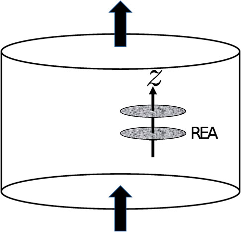
FIGURE 1. A porous plug in the form of a cylinder. There is a mixture of two immiscible fluids flowing through it in the direction of the cylinder axis under steady-state conditions. Two disks orthogonal to the cylinder axis are further imagined. These are REAs.

A central concept in the following is the representative elementary area (REA) [34, 35, 39]. We pick a point in the porous plug. In a neighborhood of this point, there will a set of streamlines associated with the velocity field ${\vec{v}}_{}$. The overall flow direction is then defined by the tangent vectors to the streamlines. We place an imaginary disk of area A at the point, with orientation such that A is orthogonal to the overall flow direction. We illustrate this as the lower disk in Figure 1. We assume that the disk is small enough for the porous medium to be homogeneous over the size of the plane with respect to porosity and permeability. This disk is an REA.

The REA will contain different fluid configurations. By “fluid configuration”, we mean the spatial distributions of the two fluids in the disk and their scalar velocity fields. We also show a second disk in Figure 1, which represents another REA placed further along the average flow. Since the flow is incompressible, we can imagine the z-axis corresponding to a pseudo-time axis. We may state that the fluid configuration in the lower disk of Figure 1 evolves into the fluid configuration in the upper disk under pseudo-time-translation. We now associate entropy to the fluid configurations in the sense of Shannon [40]. Even though the system is producing molecular entropy through dissipation, it is not producing Shannon entropy along the z-axis. This allows us to use the Jaynes maximum entropy principle, and a statistical mechanics based on Shannon entropy ensues [35].

This statistical mechanics scales up the pore-scale physics, represented by the fluid configurations to the Darcy scale, which then is represented by a thermodynamics-like formalism involving averaged velocities.

Rudiments of this thermodynamics-like formalism was first studied by Hansen et al. [32], who used extensivity to derive a set of equations that relate the seepage velocity of each of the two immiscible fluids flowing under steady state conditions through a representative volume element (REV). They introduced a co-moving velocity together with the average seepage velocity v that contained the necessary information to determine the seepage velocities of the more wetting and the less wetting fluids, v_w and v_n respectively. Stated in a different way, these equations made it possible to make the transformation

$\left(v,v_m\right)\leftrightarrows \left(v_w,v_n\right).(1)$

It is the aim of this paper to present a geometrical interpretation of the transformation in Eq. 1. We wish to provide an intuitive understanding of precisely what the transformation means and to determine the role of the co-moving velocity. Our aim is not to develop the theory presented in [32] further by including new results, but rather consolidate and amend the existing theory with a deeper understanding.

Our geometrical interpretation will rest upon the definition of a space spanned by two central variables: the wetting and non-wetting transversal pore areas. These areas are defined as the area of REAs covered by the wetting and non-wetting fluids, respectively.

Instead of using the two extensive areas directly, one often works with coordinates where one is the (wetting) saturation. If the pore area of the REA is fixed, it is often convenient to let the other variable be this area. A third way—which is new—is to use polar coordinates. This, as we shall see, simplify the theory considerably.

In Section 2, we describe the REA and the relevant variables. We define intensive and extensive variables, tying them to how they scale under scaling of the size of the REV. We also review the central results of Hansen et al. [32] here: the introduction of the auxiliary thermodynamic velocities and the co-moving velocity.

The central concept in our approach to the immiscible two-fluid flow problem is that of the pore areas. In Section 3 we introduce area space, a space that simplifies the analysis considerably. We showcase different coordinate systems on this space, focusing on polar coordinates.

Section 4 expresses the central results of Hansen et al. [32] in polar coordinates. Expressed in this coordinate system, the geometrical structure implied by the extensivity versus intensivity conditions imposes restrictions that simplify the equations. The section goes on to express the total pore velocity, seepage velocities, thermodynamic velocities, and co-moving velocity in terms of polar coordinates. This provides a clear geometrical interpretation of the co-moving velocity.

Section 5 focuses on relations between the different velocities that can be expressed without referring to any coordinate system. We do this by invoking differential forms and exterior algebra [41, 42]. Differential forms constitute the generalization of the infinitesimal line, area, or volume elements used in integrals and exterior calculus is the algebra that makes it possible to handle them. Flanders predicted in the early sixties [41] that within short they would become important tools in engineering. This did not happen, and they have remained primarily within mathematics and theoretical physics. Such objects are also especially prevalent in thermodynamics, and here, we will show that the computational rules of differential forms provide a simple way of expressing the relations between the velocities in the system at hand.

Section 6 focuses the discussion on the co-moving velocity by constructing a coordinate-independent expression that defines it.

We present in Section 7 two concrete systems. 1) A porous medium obeying the Brooks–Corey relative permeability and 2) a capillary fiber bundle model, which we analyze using the methods developed in this paper.

In Section 8, we summarize our main results which may be stated through three Eqs 58, 69, 98. These equations formulate in a coordinate-free way the three relations that exist between the average seepage velocity and the co-moving velocity.

2 Representative elementary area

We will now elaborate on the definition of the REA presented in Section 1.

We define the transversal pore area A_p as previously defined, which defines porosity

$\varphi =\frac{A_p}{A}.(2)$

The pore volume contains two immiscible fluids; the more wetting fluid (to be referred to as the wetting fluid) or the less wetting fluid (to be referred to as the non-wetting fluid). The transversal pore area A_p may, therefore, be split into the area of the REA disk cutting through the wetting fluid A_w or cutting through the non-wetting fluid A_n so that we have

$A_p=A_w+A_n.(3)$

We also define the saturations

$S_w=\frac{A_w}{A_p},(4)$

$S_n=\frac{A_n}{A_p},(5)$

so that

$S_w+S_n=1.(6)$

We note that the transversal pore areas A_p, A_w, and A_n are extensive in the REA A, that is A_p → λA_p, A_w → λA_w, and A_n → λA_n when A → λA. The porosity ϕ and the two saturations S_w and S_n are intensive in the REA A: ϕ → λ⁰ϕ, S_w → λ⁰S_w and S_n → λ⁰S_n when A → λA.

There is a time averaged volumetric flow rate Q through the REA. The volumetric flow rate consists of two components, Q_w and Q_n, which are the volumetric flow rates of the wetting and the non-wetting fluids. We have

$Q=Q_w+Q_n.(7)$

We define the total, wetting, and non-wetting seepage velocities, respectively, as

$v=\frac{Q}{A_p},(8)$

$v_w=\frac{Q_w}{A_w},(9)$

$v_n=\frac{Q_n}{A_n}.(10)$

Using Eqs 7–10, we find

$\begin{array}{ll}\hfill v& =\frac{Q}{A_p}=\frac{A_w}{A_p}\frac{Q_w}{A_w}+\frac{A_n}{A_p}\frac{Q_n}{A_n}\hfill \\ \hfill & =S_w{v}_w+S_n{v}_n.\hfill \end{array}(11)$

The volumetric flow rates Q, Q_w, and Q_n are extensive in the REA A, and the velocities v, v_w, and v_n are intensive in the area A.

2.1 Euler homogeneity

As the areas A_w and A_n, and the volumetric flow rate Q are extensive in the REA A, we have that

$Q\left(\lambda A_w,\lambda A_n\right)=\lambda Q\left(A_w,A_n\right).(12)$

This scaling was the basis for the theory presented in [32], which we now summarize.

We now apply the Euler homogeneous function theorem to Q. We take the derivative with respect to λ on both sides of Eq. 12 and set λ = 1. This gives

$Q\left(A_w,A_n\right)=A_w{\left(\frac{\partial Q}{\partial A_w}\right)}_{A_n}+A_n{\left(\frac{\partial Q}{\partial A_n}\right)}_{A_w}.(13)$

We note here that we assume A_w and A_n are our independent control variables. This makes A_p, S_w, and S_n dependent variables. More precisely, Eq. 13 is the Euler theorem for homogeneous functions applied to a degree-1 homogeneous function Q. By dividing this equation by A_p, we have

$v=S_w{\left(\frac{\partial Q}{\partial A_w}\right)}_{A_n}+S_n{\left(\frac{\partial Q}{\partial A_n}\right)}_{A_w},(14)$

where we have used Eqs 4, 5. We define the two thermodynamic velocities ${\widehat{v}}_w$ and ${\widehat{v}}_n$ as

${\widehat{v}}_w={\left(\frac{\partial Q}{\partial A_w}\right)}_{A_n}(15)$

and

${\widehat{v}}_n={\left(\frac{\partial Q}{\partial A_n}\right)}_{A_w}(16)$

so that we may write Eq. 14 as

$v=S_w{\widehat{v}}_w+S_n{\widehat{v}}_n.(17)$

The thermodynamic velocities ${\widehat{v}}_w$ and ${\widehat{v}}_n$ are not the physical velocities v_w and v_n. Rather, the most general relation between v_w and ${\widehat{v}}_w$ and v_n and ${\widehat{v}}_n$, which fulfills both Eqs 11, 17,

$v=S_w{\widehat{v}}_w+S_n{\widehat{v}}_n=S_w{v}_w+S_n{v}_n,(18)$

can be expressed as

${\widehat{v}}_w=v_w+S_n{v}_m,(19)$

${\widehat{v}}_n=v_n-S_w{v}_m.(20)$

This defines the co-moving velocity v_m, which relates the thermodynamic and the physical velocities.

We have up to now used (A_w, A_n) as our control variables. If we now consider the coordinates (S_w, A_p) instead, we can write

$\begin{array}{ll}\hfill {\widehat{v}}_w={\left(\frac{\partial Q}{\partial A_w}\right)}_{A_n}& ={\left(\frac{\partial Q}{\partial S_w}\right)}_{A_p}{\left(\frac{\partial S_w}{\partial A_w}\right)}_{A_n}+{\left(\frac{\partial Q}{\partial A_p}\right)}_{S_w}\hfill \\ \hfill & =\left(\frac{dv}{d{S}_w}\right)S_n+v,\hfill \end{array}(21)$

where we have used that

${\left(\frac{\partial S_w}{\partial A_w}\right)}_{A_n}={\left(\frac{\partial }{\partial A_w}\right)}_{A_n}\left(\frac{A_w}{A_w+A_n}\right)=\frac{S_n}{A_p}.(22)$

Likewise, we find that

${\widehat{v}}_n={\left(\frac{\partial Q}{\partial A_n}\right)}_{A_w}=-\left(\frac{dv}{d{S}_w}\right)S_w+v.(23)$

We combine Eqs 21, 23 with Eqs 19, 20 to find

$v_w=v+S_n\left(\frac{dv}{d{S}_w}-v_m\right),(24)$

$v_n=v-S_w\left(\frac{dv}{d{S}_w}-v_m\right),(25)$

and we see that these two equations give the map (v, v_m) → (v_w, v_n).

We now subtract Eq. 25 from Eq. 24, finding

$\frac{dv}{d{S}_w}=v_w-v_n+v_m,(26)$

and we now differentiate Eq. 11 with respect to S_w,

$\frac{dv}{d{S}_w}=v_w-v_n+S_w\frac{d{v}_w}{d{S}_w}+S_n\frac{d{v}_n}{d{S}_w}.(27)$

We compare Eqs 26, 27, finding

$v_m=S_w\frac{d{v}_w}{d{S}_w}+S_n\frac{d{v}_n}{d{S}_w}.(28)$

Eqs 11, 28 constitute the inverse mapping (v_w, v_n) → (v, v_m).

The mapping (v, v_m) → (v_w, v_n) tells us that given the constitutive equations for v and v_m, we also have the constitutive equations for v_w and v_n. It turns out that the constitutive equation for v_m is surprisingly simple [34],

$v_m=a+b\frac{dv}{d{S}_w},(29)$

where a and b are coefficients depending on the entropy associated with the fluid configurations [35].

The equations we have used in Section 2 hint at an underlying mathematical structure which may seem complex. As we will now show, it is in fact quite the opposite.

3 Coordinate systems in area space

The transversal pore areas A_w ≥ 0 and A_n ≥ 0 parametrize the first quadrant of ${\mathbb{R}}^2$. This serves as the “area space” mentioned earlier, which we will continue to denote as such. It is important to realize that this space is not physical space. A value of the transversal pore area A_p corresponds to a point $\left(A_w,A_n\right)$ in this space. If we consider the entire plane ${\mathbb{R}}^2$ as a whole and simply restrict our attention to the first quadrant, we may treat the area space as a vector space. The point $\left(A_w,A_n\right)$ may then equivalently be described by a vector,

$\vec{A}=A_w{\vec{e}}_w+A_n{\vec{e}}_n,(30)$

where ${\vec{e}}_w$ and ${\vec{e}}_n$ form an orthonormal basis set, shown in the leftmost figure in Figure 2. Note that in this picture, the bases are shown as attached to the point $\left(A_w,A_n\right)$. We reiterate that both A_w and A_n are extensive.

FIGURE 2

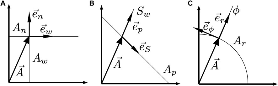
FIGURE 2. Three coordinate systems are illustrated and used to parametrize the transversal pore area. (A) The Cartesian coordinate system (A_w, A_n). A curve of constant A_w and A_n is indicated as A_w and A_n, respectively. Both A_w and A_n are extensive. The orthonormal basis set $({\vec{e}}_w,{\vec{e}}_n)$ is shown as attached to the point $\left(A_w,A_n\right)$. (B) The saturation coordinate system $\left(A_p,S_w\right)$. Curves of constant A_p and S_w are denoted by A_p and S_w in the figure. A_p is extensive and S_w is intensive. The non-orthonormal basis $({\vec{e}}_p,{\vec{e}}_s)$ is shown. (C) The polar coordinate system (A_r,φ). Curves of constant A_r and φ are denoted by A_r and φ in the figure. A_r is extensive and ϕ is intensive. The basis set $({\vec{e}}_r,{\vec{e}}_{\varphi })$ is orthonormal. In all three figures, the transversal pore area as a vector $\vec{A}$ is shown.

Every point in the transversal area space corresponds to a given saturation S_w and a transversal pore area A_p and we may view the map (A_w, A_n) → (A_p, S_w) given by Eqs 3, 4 as a coordinate transformation. This is a more natural coordinate system to work with since S_w is an intensive variable and A_p is in practice kept constant. We name this system the saturation coordinate system. We show the normalized basis vector set in the middle figure in Figure 2. We calculate

${\vec{u}}_p={\left(\frac{\partial \vec{A}}{\partial A_p}\right)}_{S_w}=S_w{\vec{e}}_w+\left(1-S_w\right){\vec{e}}_n,(31)$

${\vec{u}}_s={\left(\frac{\partial \vec{A}}{\partial S_w}\right)}_{A_p}=A_p{\vec{e}}_w-A_p{\vec{e}}_n.(32)$

We normalize the two vectors ${\vec{u}}_p$ and ${\vec{u}}_s$ to find

${\vec{e}}_p=\frac{S_w{\vec{e}}_w+\left(1-S_w\right){\vec{e}}_n}{{\left[1-2S_w\left(1-S_w\right)\right]}^{1/2}},(33)$

${\vec{e}}_s=\frac{{\vec{e}}_w-{\vec{e}}_n}{\sqrt{2}}.(34)$

This basis set is not orthonormal, as illustrated in Figure 2. By expressing $\vec{A}$ in this coordinate system, we find

$\vec{A}=A_p{\left[1-2S_w\left(1-S_w\right)\right]}^{1/2}{\vec{e}}_p.(35)$

As it will become apparent, the most convenient coordinate system to work with from a theoretical point of view is polar coordinates $\left(A_r,\varphi \right)$, given by

$A_r=\sqrt{A_w^2+A_n^2},(36)$

$\varphi =\arctan \left(\frac{A_n}{A_w}\right),(37)$

or vice versa.

$A_w=A_r\cos \varphi ,(38)$

$A_n=A_r\sin \varphi .(39)$

We note that ϕ is intensive and A_r is extensive. We show the polar coordinate system in the lower figure in Figure 2.

The basis vector set $({\vec{e}}_r,{\vec{e}}_{\varphi })$ is orthonormal, where

${\vec{e}}_r=\cos \varphi {\vec{e}}_w+\sin \varphi {\vec{e}}_n={\vec{e}}_p,(40)$

${\vec{e}}_{\varphi }=-\sin \varphi {\vec{e}}_w+\cos \varphi {\vec{e}}_n.(41)$

As for the saturation coordinate system, there is one intensive variable, ϕ, and one extensive variable, A_r. However, in contrast to the saturation coordinate system, both variables are varied in practical situations.

We have that

$\vec{A}=A_r{\vec{e}}_r.(42)$

We see that this is consistent with Eq. 35 since

$A_r=A_p{\left[1-2S_w\left(1-S_w\right)\right]}^{1/2}(43)$

and ${\vec{e}}_p={\vec{e}}_r$.

4 Euler homogeneity in polar coordinates

We now focus on Eq. 12 which we repeat here.

$Q\left(\lambda A_w,\lambda A_n\right)=\lambda Q\left(A_w,A_n\right).$

We may interpret this equation geometrically. If we follow the value of Q along a ray passing through the origin of the two-dimensional space spanned by (A_w, A_n) keeping the ratio A_n/A_w constant, it grows linearly with the distance from the Q-axis.

In polar coordinates, this means

$Q\left(A_r,\varphi \right)={\widehat{v}}_r{A}_r,(44)$

where

${\widehat{v}}_r={\left(\frac{\partial Q}{\partial A_r}\right)}_{\varphi }={\widehat{v}}_r\left(\varphi \right).(45)$

The important point here is that ${\widehat{v}}_r$ is not a function of A_r.

We may derive Eq. 44 from Eq. 12 as follows. First, we write A_w and A_n in terms of A_r and ϕ in Eq. 12 so that

$\begin{array}{ll}\hfill & \frac{1}{\lambda }Q\left(\lambda A_r\cos \varphi ,\lambda A_r\sin \varphi \right)\hfill \\ \hfill & =Q\left(A_r\cos \varphi ,A_r\sin \varphi \right)=Q\left(A_r,\varphi \right).\hfill \end{array}(46)$

Next, we set λ = 1/A_r to find

$A_{r}Q\left(\cos \varphi ,\sin \varphi \right)=A_r{\widehat{v}}_r\left(\varphi \right)=Q\left(A_r,\varphi \right),(47)$

where

${\widehat{v}}_r\left(\varphi \right)\equiv Q\left(\cos \varphi ,\sin \varphi \right),(48)$

and we are done. We illustrate in Figure 3 the geometrical meaning of Eq. 12, that is, Euler homogeneity. The graph of the volumetric flow rate Q takes the shape of a “crumpled” cone in the space spanned by (Q, A_w, A_n).

FIGURE 3

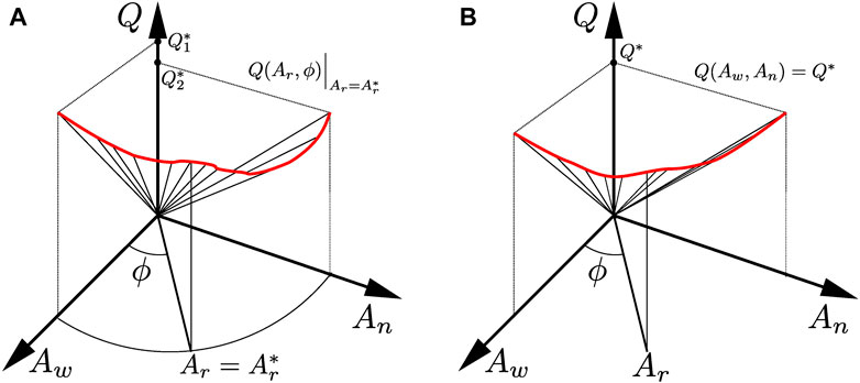
FIGURE 3. Geometrical meaning of the function Q being degree-1 Euler homogeneous in the extensive variables, meaning it fulfils equation (12), using polar coordinates. We here use the same symbol Q as both a variable and a function. Moving along a ray in the space spanned by the variables Q, A_w and A_n, the volumetric flow rate increases linearly with the distance from the Q-axis. For a constant value $A_r^{\ast }$ of the radial coordinate A_r (A) or a constant value Q^∗ of the volumetric flow rate (B), the graph of Q appears as a “crumpled” cone originating at the origin, with the level set (shown in red) imagined as an “edge”. The level sets are different in the two cases. In particular, the volumetric flow rate will in (A) have different limiting values $Q_1^{\ast }$ and $Q_2^{\ast }$ in the limit of single-phase flow of either the wetting or non-wetting fluid.

We now express the different fluid velocities, namely the pore velocity, seepage velocities, thermodynamic velocities, and the co-moving velocity, in terms of polar coordinates.

4.1 Seepage velocities

The area space spanned by $\left(A_w,A_n\right)$ is simply (a subset of) the real plane. We can therefore identify it with the tangent space of velocities, which is the same Cartesian plane as that of the areas $\left(A_w,A_n\right)$. We can therefore regard the seepage velocity as a vector in the area space,

$\vec{v}=v_w{\vec{e}}_w+v_n{\vec{e}}_n.(49)$

The volumetric flow rate Q is then given by the scalar product

$Q=\vec{v}\cdot \vec{A}=v_w{A}_w+v_n{A}_n={\widehat{v}}_w{A}_w+{\widehat{v}}_n{A}_n.(50)$

In polar coordinates, the seepage velocity is given by

$\vec{v}=v_r{\vec{e}}_r+v_{\varphi }{\vec{e}}_{\varphi }.(51)$

Hence, the volumetric flow rate in polar coordinates is given by

$Q=\vec{v}\cdot \vec{A}=\left(v_r{\vec{e}}_r+v_{\varphi }{\vec{e}}_{\varphi }\right)\cdot \left(A_r{\vec{e}}_r\right)=v_r{A}_r.(52)$

Comparing with Eq. 44, we find

$v_r={\widehat{v}}_r={\widehat{v}}_r\left(\varphi \right).(53)$

By using Eqs 49, 51 combined with Eqs 40, 41, we find

$\begin{array}{ll}\hfill v_r& =v_w\cos \varphi +v_n\sin \varphi \hfill \\ \hfill & =\frac{S_w{v}_w+\left(1-S_w\right)v_n}{{\left[1-2S_w\left(1-S_w\right)\right]}^{1/2}},\hfill \end{array}(54)$

$\begin{array}{ll}\hfill v_{\varphi }& =-v_w\sin \varphi +v_n\cos \varphi \hfill \\ \hfill & =\frac{-\left(1-S_w\right)v_w+S_w{v}_n}{{\left[1-2S_w\left(1-S_w\right)\right]}^{1/2}}.\hfill \end{array}(55)$

We have here expressed cos ϕ and sin ϕ in terms of S_w.

We now compare Eq. 44 with Eq. 8, rewritten as

$Q=v{A}_p.(56)$

Using Eq. 43, we find that their equality demands

$v=\frac{{\widehat{v}}_r}{{\left[1-2S_w\left(1-S_w\right)\right]}^{1/2}}.(57)$

Hence, v is not the norm of $\vec{v}$.

4.2 Thermodynamic velocities

We may write Eq. 13 as

$Q={\widehat{v}}_w{A}_w+{\widehat{v}}_n{A}_n=\widehat{\vec{v}}\cdot \vec{A},(58)$

where we have defined, in the same manner as for Eq. 49,

$\widehat{\vec{v}}={\widehat{v}}_w{\vec{e}}_w+{\widehat{v}}_n{\vec{e}}_n.(59)$

We use Eqs 40, 41 to express this equation in polar coordinates,

$\widehat{\vec{v}}={\widehat{v}}_r{\vec{e}}_r+{\widehat{v}}_{\varphi }{\vec{e}}_{\varphi },(60)$

where

${\widehat{v}}_r={\widehat{v}}_w\cos \varphi +{\widehat{v}}_n\sin \varphi ,,(61)$

${\widehat{v}}_{\varphi }=-{\widehat{v}}_w\sin \varphi +{\widehat{v}}_n\cos \varphi .(62)$

4.3 Co-moving velocity

We defined the co-moving velocity v_m as the velocity function that relates the physical seepage velocities and the thermodynamic velocities shown in Eqs 19, 20. We use these two equations together with Eqs 49, 59 to form the vector

$\begin{array}{ll}\hfill \widehat{\vec{v}}-\vec{v}& =\left({\widehat{v}}_w-v_w\right){\vec{e}}_w+\left({\widehat{v}}_n-v_n\right){\vec{e}}_n\hfill \\ \hfill & =\frac{v_m}{A_p}\left(A_n{\vec{e}}_w-A_w{\vec{e}}_n\right)\hfill \\ \hfill & =\frac{v_m}{A_p}\left(A_r\sin \varphi {\vec{e}}_w-A_r\cos \varphi {\vec{e}}_n\right),\hfill \end{array}(63)$

where we have used S_w = A_w/A_p and Eqs 38, 39. We rewrite this equation in terms of ${\vec{e}}_{\varphi }$, Eq. 41, finding

$\widehat{\vec{v}}-\vec{v}=-\frac{v_m}{\cos \varphi +\sin \varphi }{\vec{e}}_{\varphi }.(64)$

We define

${\widehat{v}}_m=\frac{v_m}{\cos \varphi +\sin \varphi }(65)$

so that Eq. 63 may be written as

$\vec{v}=\widehat{\vec{v}}+{\widehat{\vec{v}}}_m,(66)$

where

${\widehat{\vec{v}}}_m={\widehat{v}}_m{\vec{e}}_{\varphi }.(67)$

In polar coordinates, the relation in Eq. 66 is isolated to the ϕ-coordinate. Using Eqs 51, 62, we can express the relation between the vector components ${\widehat{v}}_{\varphi }$ and v_ϕ as

$v_{\varphi }={\widehat{v}}_{\varphi }+{\widehat{v}}_m.(68)$

We illustrate this relation in Figure 4. This figure also demonstrates why $Q=\widehat{\vec{v}}\cdot \vec{A}=\vec{v}\cdot \vec{A}$; it is due to $(\vec{v}-\widehat{\vec{v}})={\widehat{\vec{v}}}_m\perp \vec{A}$. Hence, we have that

${\widehat{\vec{v}}}_m\cdot \vec{A}=0.(69)$

FIGURE 4

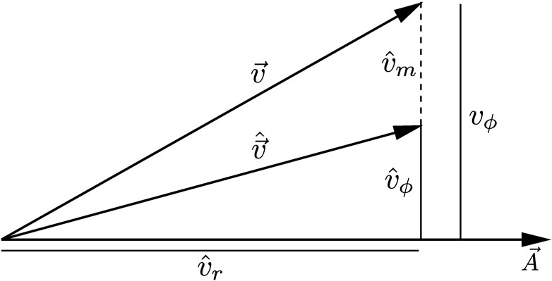
FIGURE 4. Vectorial representation for eqs. 52, 58, where $A_r=|\vec{A}|$ is illustrated. The difference in the vectors $\widehat{\vec{v}}$ and $\vec{v}$, ${\widehat{v}}_m$, is orthogonal to $\vec{A}$, and cannot be detected by the properties of $\vec{A}$ alone.

5 Coordinate-free representation

Since the difference between the thermodynamic- and seepage velocities in the previous section was shown to sit in the tangent vector components, we can benefit from examining the problem from a position where these components are easier to work with. In this section, we therefore introduce differential forms and exterior algebra [41, 42] to make this treatment more economic. In addition, this makes it easier to formulate the equations met so far in a way that does not depend on the coordinate system used.

Eq. 44, $Q={\widehat{v}}_r{A}_r$, may be differentiated to give

$dQ={\widehat{v}}_{r}d{A}_r+d{\widehat{v}}_r{A}_r={\widehat{v}}_{r}d{A}_r+{\widehat{v}}_r^{\prime }{A}_{r}d\varphi ,(70)$

where ${\widehat{v}}_r^{\prime }=d{\widehat{v}}_r/d\varphi$. Here, dQ, dA_r, and dϕ are one-forms. Furthermore, we have that

$\begin{array}{ll}\hfill dQ& ={\left(\frac{\partial Q}{\partial A_r}\right)}_{\varphi }d{A}_r+{\left(\frac{\partial Q}{\partial \varphi }\right)}_{A_r}d\varphi \hfill \\ \hfill & ={\widehat{v}}_{r}d{A}_r+{\widehat{v}}_{\varphi }{A}_{r}d\varphi .\hfill \end{array}(71)$

Comparing Eqs 70, 71 gives

${\widehat{v}}_{\varphi }={\widehat{v}}_r^{\prime }.(72)$

We do the same using the coordinate system (A_w, A_n). From Eq. 50, we find

$\begin{array}{ll}\hfill dQ& ={\widehat{v}}_{w}d{A}_w+{\widehat{v}}_{n}d{A}_n+A_{w}d{\widehat{v}}_w+A_{n}d{\widehat{v}}_n\hfill \\ \hfill & ={\widehat{v}}_{w}d{A}_w+{\widehat{v}}_{n}d{A}_n.\hfill \end{array}(73)$

In the second equality, we assumed that dQ is an exact differential, and in the first equality, we applied the differential to $Q={\widehat{v}}_w{A}_w+{\widehat{v}}_n{A}_n$. This implies the relation

$A_{w}d{\widehat{v}}_w+A_{n}d{\widehat{v}}_n=0.(74)$

This equation corresponds to the Gibbs–Duhem equation in thermodynamics, which is a statement of the dependency amongst the intensive variables.

We express ${\widehat{v}}_w$ and ${\widehat{v}}_n$ in terms of ${\widehat{v}}_r$ and ${\widehat{v}}_{\varphi }$ by inverting Eqs 61, 62 to find

${\widehat{v}}_w={\widehat{v}}_r\cos \varphi -{\widehat{v}}_{\varphi }\sin \varphi ,,(75)$

${\widehat{v}}_n={\widehat{v}}_r\sin \varphi +{\widehat{v}}_{\varphi }\cos \varphi .(76)$

By applying the exterior derivative, we get the relations

$d{\widehat{v}}_w=\cos \varphi d{\widehat{v}}_r-\sin \varphi d{\widehat{v}}_{\varphi }-{\widehat{v}}_{n}d\varphi ,(77)$

$d{\widehat{v}}_n=\sin \varphi d{\widehat{v}}_r+\cos \varphi d{\widehat{v}}_{\varphi }+{\widehat{v}}_{w}d\varphi .(78)$

Combining Eqs 75–78 with Gibbs–Duhem Eq. 74 gives

$\frac{d{\widehat{v}}_r}{d\varphi }={\widehat{v}}_{\varphi },(79)$

which is identical to Eq. 72. Hence, this is the Gibbs–Duhem equation in polar coordinates.

The thermodynamic velocity, Eq. 59, is, therefore, given by

$\widehat{\vec{v}}={\widehat{v}}_r{\vec{e}}_r+{\widehat{v}}_r^{\prime }{\vec{e}}_{\varphi }.(80)$

We now have one of the main results of Hansen et al. [32] in a very compact form.

$\vec{v}={\widehat{v}}_r{\vec{e}}_r+\left({\widehat{v}}_r^{\prime }+{\widehat{v}}_m\right){\vec{e}}_{\varphi }.(81)$

We note that since ${\widehat{v}}_r$ only depends on ϕ, the same must be true for ${\widehat{v}}_m$. Hence, ${\widehat{v}}_m={\widehat{v}}_m(\varphi )$. Here, we see that the relation between the thermodynamic- and seepage velocities are not captured in the extensive structure tied to the radial coordinate, but instead in the intensive quantities which only has a dependency on ϕ.

We now differentiate Eq. 56, $Q=\vec{v}\cdot \vec{A}$ written in the saturation coordinate system, to find

$dQ=vd{A}_p+\frac{dv}{d{S}_w}{A}_{p}d{S}_w.(82)$

We note that

$d{A}_p=d{A}_w+d{A}_n,(83)$

from differentiating Eq. 3. Likewise, we note that

$\begin{array}{ll}\hfill d{S}_w& ={\left(\frac{\partial S_w}{\partial A_w}\right)}_{A_n}d{A}_w+{\left(\frac{\partial S_w}{\partial A_n}\right)}_{A_w}d{A}_n\hfill \\ \hfill & =\frac{1}{A_p^2}\left(A_{n}d{A}_w-A_{w}d{A}_n\right),\hfill \end{array}(84)$

using Eq. 4. We combine Eqs 82–84 and find

$dQ=\left(v+\left(1-S_w\right)\frac{dv}{d{S}_w}\right)d{A}_w+\left(v-S_w\frac{dv}{d{S}_w}\right)d{A}_n.(85)$

By using Eq. 13, definitions of Eqs 15, 16, and transformations Eqs 19, 20, we may write

$\begin{array}{ll}\hfill dQ& ={\widehat{v}}_{w}d{A}_w+{\widehat{v}}_{n}d{A}_n=\left(v_w-\left(1-S_w\right)v_m\right)d{A}_w\hfill \\ \hfill & +\left(v_n+S_w{v}_m\right)d{A}_n.\hfill \end{array}(86)$

Equating Eq. 85 and Eq. 86 gives Eqs 24, 25.

Let us now rewrite the differential dQ as follows:

$\begin{array}{ll}\hfill dQ& =d\left[A_{p}v\right]=d\left[A_p\left(S_w{\widehat{v}}_w+\left(1-S_w\right){\widehat{v}}_n\right)\right]\hfill \\ \hfill & =A_p\left({\widehat{v}}_w-{\widehat{v}}_n\right)d{S}_w+vd{A}_p,\hfill \end{array}(87)$

where we have used Eq. 74. We now combine this equation with Eq. 82 to get

$\frac{dv}{d{S}_w}={\widehat{v}}_w-{\widehat{v}}_n.(88)$

By using Eqs 19, 20, we may rewrite this equation in terms of the seepage velocities, resulting in Eq. 26.

We differentiate Q a second time, which is zero according to the Poincaré lemma [41, 42]. We see that this is indeed so by using Eq. 70,

$\begin{array}{ll}\hfill d^{2}Q& =d\left({\widehat{v}}_{r}d{A}_r+{\widehat{v}}_r^{\prime }{A}_{r}d\varphi \right)\hfill \\ \hfill & ={\widehat{v}}_r^{\prime }\left(d\varphi \wedge d{A}_r\right)+{\widehat{v}}_r^{\prime }\left(d{A}_r\wedge d\varphi \right)\hfill \\ \hfill & =\left({\widehat{v}}_r^{\prime }-{\widehat{v}}_r^{\prime }\right)d\varphi \wedge d{A}_r=0,\hfill \end{array}(89)$

where the wedge ∧ signifies the antisymmetric exterior product.

The same equation expressed in the coordinate system (A_w, A_n) gives

$\begin{array}{ll}\hfill d^{2}Q& =d\left({\widehat{v}}_{w}d{A}_w+{\widehat{v}}_{n}d{A}_n\right)\hfill \\ \hfill & =\left[{\left(\frac{\partial {\widehat{v}}_n}{\partial A_w}\right)}_{A_n}-{\left(\frac{\partial {\widehat{v}}_w}{\partial A_n}\right)}_{A_n}\right]d{A}_w\wedge d{A}_n\hfill \\ \hfill & =0.\hfill \end{array}(90)$

We rewrite the coefficient in terms of the saturation coordinate system,

$\begin{array}{ll}\hfill {\left(\frac{\partial {\widehat{v}}_n}{\partial A_w}\right)}_{A_n}-{\left(\frac{\partial {\widehat{v}}_w}{\partial A_n}\right)}_{A_n}& =\hfill \\ \hfill \frac{d{\widehat{v}}_n}{d{S}_w}{\left(\frac{\partial S_w}{\partial A_w}\right)}_{A_n}-\frac{d{\widehat{v}}_w}{d{S}_w}{\left(\frac{\partial S_w}{\partial A_n}\right)}_{A_w}& =\hfill \\ \hfill S_w\frac{d{\widehat{v}}_w}{d{S}_w}+\left(1-S_w\right)\frac{d{\widehat{v}}_n}{d{S}_w}& =0,\hfill \end{array}(91)$

which is nothing but the Gibbs–Duhem equation yet again. Writing this equation in terms of the seepage velocities gives us Eq. 28.

We see that the different equations relating the velocities can all be found from the differential geometric structure of the space spanned by the areas, with addition to Euler homogeneity, see Figure 3. All relations are either a consequence of writing dQ using different coordinate systems or a consequence of the Poincaré lemma, expressed as d²Q = 0.

6 The co-moving velocity in coordinate-free representation

The co-moving velocity appears in several equations in the previous sections. Common to all of them is that they all are written out in terms of a given coordinate system. We may write the representation of the co-moving velocity in the saturation coordinate system, Eq. 28, as

$A_p{v}_m=\vec{A}\cdot \frac{d\vec{v}}{d{S}_w}.(92)$

We may write Eq. 65 in polar coordinates as

$A_r{\widehat{v}}_m=-\vec{A}\cdot \frac{d\vec{v}}{d\varphi }.(93)$

Expressed in terms of the seepage velocities, we have that

$dQ=v_{w}d{A}_w+v_{n}d{A}_n+A_{w}d{v}_w+A_{n}d{v}_n.(94)$

In order to obtain an expression for the co-moving velocity which is independent of the coordinate system, we construct

$\begin{array}{ll}\hfill A_{w}d{v}_w+A_{n}d{v}_n& =v_m\frac{A_{n}d{A}_w-A_{w}d{A}_n}{A_w+A_n}\hfill \\ \hfill & =v_m{A}_{p}d{S}_w=-{\widehat{v}}_m{A}_{r}d\varphi ,\hfill \end{array}(95)$

where the second line only reflects Eqs 92, 93.

We write dQ as

$dQ=d\left[\vec{A}\cdot \widehat{\vec{v}}\right]={\widehat{v}}^{i}d{A}_i,(96)$

using Eq. 74. Here, Einstein summation convention has been applied, with the index i running over $\left\{w,n\right\}$ in the basis $\left(A_w,A_n\right)$. In terms of the seepage velocities, this becomes

$dQ=d\left[\vec{A}\cdot \vec{v}\right]=v^{i}d{A}_i+A^{i}d{v}_i.(97)$

Combining Eqs 96, 97, 66 gives us

${\widehat{v}}_m^{i}d{A}_i+A^{i}d{v}_i=0,(98)$

where ${\widehat{v}}_m^i$ denotes the components of ${\widehat{\vec{v}}}_m$. This holds in any coordinate system, since it is just obtained by differentiating a function, namely $\vec{A}\cdot \vec{v}$. We have, therefore, obtained an expression for the co-moving velocity which is independent of the chosen coordinate system.

We can introduce vector-valued differential forms [42] to make a connection between the interpretation in terms of (tangent) vectors used up until now and the language of differential forms. Let $\left\{{\vec{e}}_i\right\}$ be an arbitrary basis for vectors on the area space as we have discussed until now, be it area-, saturation-, or polar coordinates. We now take $\vec{A}$ as an example. We write

$A={\beta }^i{\vec{e}}_i,(99)$

where we have applied the Einstein summation convention. A is now regarded as a vector-valued differential form (thus seeing ${\vec{e}}_i$ as components written out in the βⁱ basis, i.e., a reversal of viewpoint), the βⁱ are 0-forms, just functions, and the index i runs over the coordinate indices. We can still treat A as a vector, but the difference in viewpoints is apparent when we apply the exterior derivative d to A, which gives

$dA={\displaystyle \sum _i}\left({{\displaystyle \vec{e}}}_i\otimes d{\beta }_i\right)=\left(d{\beta }^i\right){{\displaystyle \vec{e}}}_i,(100)$

where we have suppressed the tensor product of the forms and basis vectors since we are working over a vector space, as is standard notation in for example [42]. Strictly speaking, the exterior derivative d should be replaced by the exterior covariant derivative in this setting, a generalization of d which is defined on both tangent vectors and forms (there is currently no term in Eq. 100 that reflect the changes in the basis ${\vec{e}}_i$). The terms Aⁱdv_i are then possible to interpret in terms of connection forms. However, this is outside the scope of the current discussion, and we leave this topic for future work.

If we write out Eq. 100 in the coordinate system $\left(A_w,A_n\right)$, we get

$dA=d{A}_w{\vec{e}}_w+d{A}_n{\vec{e}}_n.(101)$

With this formalism in mind, we now return to polar coordinates. Eq. 98 may be written in these coordinates by using Eqs 40, 41 to define the vector valued 0-forms,

${\omega }_r=\cos \varphi {\vec{e}}_w+\sin \varphi {\vec{e}}_n,,(102)$

${\omega }_{\varphi }=-\sin \varphi {\vec{e}}_w+\cos \varphi {\vec{e}}_n,(103)$

which are equivalent to the corresponding basis vectors in Eqs 40, 41, but interpreted as 0-forms. We then compute

$d{\omega }_r={\vec{e}}_{\varphi }d\varphi ,,(104)$

$d{\omega }_{\varphi }=-{\omega }_{r}d\varphi (105)$

so that

$\begin{array}{ll}\hfill dA=d\left(A_r{\omega }_r\right)& =d{A}_r{\omega }_r+A_{r}d{\omega }_r\hfill \\ \hfill & =d{A}_r{\vec{e}}_r+A_r{\vec{e}}_{\varphi }d\varphi ,\hfill \end{array}(106)$

where in the second equality, we have used ω_r which is just another way of writing the basis vector ${\vec{e}}_r$ that emphasizes its role as a form.

We can similarly define vector valued 1-forms $d\widehat{v}$ and dv from Eqs 59, 49 respectively. We then straightforwardly obtain

$d\widehat{v}=d{\widehat{v}}_w{\vec{e}}_w+d{\widehat{v}}_n{\vec{e}}_n,,(107)$

$dv=d{v}_w{\vec{e}}_w+d{v}_n{\vec{e}}_n.(108)$

We express dv in polar coordinates as

$\begin{array}{ll}\hfill dv& =v_r^{\prime }{\vec{e}}_{r}d\varphi +v_r{\vec{e}}_{\varphi }d\varphi +v_{\varphi }^{\prime }{\vec{e}}_{\varphi }d\varphi -v_{\varphi }{\vec{e}}_{r}d\varphi \hfill \\ \hfill & =\left[\left(v_r^{\prime }-v_{\varphi }\right){\vec{e}}_r+\left(v_r+v_{\varphi }^{\prime }\right){\vec{e}}_{\varphi }\right]d\varphi ,\hfill \end{array}(109)$

giving

$A_r{\widehat{v}}_{m}d\varphi =A_r\left(v_{\varphi }-v_r^{\prime }\right)d\varphi ,(110)$

or

${\widehat{v}}_m=v_{\varphi }-v_r^{\prime }.(111)$

By combining Eqs 54, 68, 72, we obtain the same equation. Eq. 98 written in the saturation coordinate system yields Eq. 28.

7 Applications

We give in this section a couple of examples of practical use of the ideas that have been presented. We consider first the Brooks–Corey relative permeability model [43] and then a capillary fiber bundle model [44, 45].

7.1 The brooks–corey model

We assume an irreducible wetting fluid saturation S_w,i and residual non-wetting fluid saturation S_n,r so that S_w,i ≤ S_w ≤ 1 − S_n,r and S_n,r ≤ S_n ≤ 1 − S_w,i. We renormalize the saturations to be

$S_w^{*}=\frac{S_{nw}-S_{n,r}}{1-S_{w,i}-S_{n,r}},(112)$

$S_n^{*}=\frac{S_w-S_{w,i}}{1-S_{w,i}-S_{n,r}}.(113)$

The Brooks–Corey relative permeability is [43]

$k_{rw}=k_{rw}^0{\left(S_w^{*}\right)}^{n_w},(114)$

$k_{rn}=k_{rn}^0{\left(S_n^{*}\right)}^{n_n},(115)$

The seepage velocities are

$v_w=-\frac{K{k}_{rw}^0}{\phi {\mu }_w}{\left(S_w^{*}\right)}^{n_w-1}\nabla P\equiv M_w{\left(S_w^{*}\right)}^{n_w-1},(116)$

$v_n=-\frac{K{k}_{rn}^0}{\phi {\mu }_n}{\left(S_n^{*}\right)}^{n_n-1}\nabla P\equiv M_n{\left(S_n^{*}\right)}^{n_n-1}.(117)$

Here, K is the absolute permeability, φ is the porosity, and μ_w and μ_n are the viscosities. We assume no gradients in the saturation so that no capillary pressure enters, only the pressure P.

We find the average seepage velocity to be

$v=M_w{\left(S_w^{*}\right)}^{n_w}+M_n{\left(S_n^{*}\right)}^{n_n}(118)$

and the co-moving velocity to be

$v_m=\left(n_w-1\right)M_w{\left(S_w^{*}\right)}^{n_w-1}-\left(n_n-1\right)M_n{\left(S_n^{*}\right)}^{n_w-1}.(119)$

We also note that

$\frac{dv}{d{S}_w^{*}}=n_w{M}_w{\left(S_w^{*}\right)}^{n_w-1}-n_n{M}_n{\left(S_n^{*}\right)}^{n_w-1}.(120)$

Hence, if n_w = n_n = n, we get

$v_m=\frac{n-1}{n}\frac{dv}{d{S}_w^{*}},(121)$

a result which is consistent with the observations in Roy et al. [34], see Eq. 29. In the following, we assume that n_w = n_n = n. This is in accordance with the findings in [46, 47], where in addition was suggested that n_w = n_n = 2. We will simplify the notation for the saturation $S_w^{*}\to S_w$ and $S_n^{*}\to S_n$.

We find from Eqs 54, 55 that the seepage velocities are in polar coordinates.

$v_r=M_w{\left(\frac{\cos \varphi }{\cos \varphi +\sin \varphi }\right)}^n\cos \varphi +M_n{\left(\frac{\sin \varphi }{\cos \varphi +\sin \varphi }\right)}^n\sin \varphi ,(122)$

$v_{\varphi }=-M_w{\left(\frac{\cos \varphi }{\cos \varphi +\sin \varphi }\right)}^n\sin \varphi +M_n{\left(\frac{\sin \varphi }{\cos \varphi +\sin \varphi }\right)}^n\cos \varphi .(123)$

We find the thermodynamic velocities in polar coordinates using Eqs 53, 79,

${\widehat{v}}_r=v_r=M_w{\left(\frac{\cos \varphi }{\cos \varphi +\sin \varphi }\right)}^n\cos \varphi +M_n{\left(\frac{\sin \varphi }{\cos \varphi +\sin \varphi }\right)}^n\sin \varphi (124)$

and

${\widehat{v}}_{\varphi }=\frac{d{\widehat{v}}_r}{d\varphi }=n\frac{\csc \varphi \sec \varphi }{\cos \varphi +\sin \varphi }{v}_{\varphi }.(125)$

Finally, from Eq. 81, we find the co-moving velocity in polar coordinates,

${\widehat{v}}_m=\left[1-n\frac{\csc \varphi \sec \varphi }{\cos \varphi +\sin \varphi }\right]v_{\varphi }.(126)$

7.2 Capillary fiber bundle model

We now turn to the capillary fiber bundle model [44, 45] which serves as a rudimentary model of a porous medium. We will revisit a version of the model that has already been discussed by Hansen et al. [32]. Consider a bundle of N capillary tubes, all of length L. Some fraction of the tubes has a cross-sectional area a_s and the rest has a cross-sectional area a_l. We assume a_l > a_s. The total pore areas of the small and large capillary tubes are denoted A_s and A_l, respectively. These two areas sum up to the total pore area A_p,

$A_s+A_l=A_p.(127)$

We assume that the thinnest capillaries are so narrow that the non-wetting fluid may not penetrate them. Hence, the saturation due to the wetting fluid in these capillaries is irreducible, and we have

$A_s=S_{w,i}{A}_p.(128)$

Furthermore, we assume that each capillary is either fully filled with the wetting fluid or the non-wetting fluid, but never a mixture.

In the following, we sketch the analysis of Hansen et al. [32]. The wetting area A_w is then

$A_w=S_{w,i}{A}_p+\left(S_w-S_{w,i}\right)A_p=A_s+A_{lw},(129)$

where we define A_lw ≡ (S_w − S_w,i)A_p, the total wetting area in the larger capillaries. The seepage velocity of the wetting fluid in the smaller and larger capillaries is denoted v_sw and v_lw respectively. The non-wetting fluid only flows in the larger capillaries. Its seepage velocity is denoted by v_n, and the saturation of the non-wetting fluid is given by S_n. The total seepage velocity v is then

$v=S_{w,i}{v}_{sw}+\left(S_w-S_{w,i}\right)v_{lw}+S_n{v}_n,(130)$

where we have 0 ≤ S_n ≤ 1 − S_w,i. We multiply both sides of the equation by A_p to obtain the associated volumetric flow rate Q,

$Q=A_{p}v=A_s{v}_{sw}+A_{lw}{v}_{lw}+A_n{v}_n.(131)$

To find the co-moving velocity v_m, one can explicitly compute the thermodynamic velocities in Eq. 15 or Eq. 16, and use the relations between the thermodynamic- and seepage velocities, Eq. 19 and Eq. 20. The resulting co-moving velocity for this system can then be shown [32] to be

$v_m=\frac{S_{w,i}}{S_w}\left(v_{lw}-v_{sw}\right).(132)$

We note that these expressions are fairly complicated. This is due to the choice of origin of the coordinate system, namely S_w = 0 and A_p = 0. It is convenient to shift the origin from (S_w, A_p) = (0, 0) to (S_w,i, A_s), as conducted in Section 7.1. Hence, we define $S_w^{*}=S_w-S_{w,i}$, $A_p^{*}=A_p-A_s$, and $A_w^{*}=A_w-A_s$. We immediately drop the star superscripts in these expressions.

We find the thermodynamic velocities easily,

${\widehat{v}}_w={\left(\frac{\partial Q}{\partial A_w}\right)}_{A_n}=v_{lw},(133)$

${\widehat{v}}_n={\left(\frac{\partial Q}{\partial A_n}\right)}_{A_w}=v_n.(134)$

The wetting volumetric flow rate is

$Q_w=A_p{S}_{w,i}{v}_{sw}+A_w{v}_{lw}.(135)$

We subtract the volumetric flow rate due to the irreducible wetting fluid.

$Q_w^{*}=Q_w-A_p{S}_{w,i}{v}_{sw}=A_s{v}_{lw}\to Q_w.(136)$

The seepage velocity vector then becomes

$\vec{v}=v_{lw}{\vec{e}}_w+v_n{\vec{e}}_n.(137)$

The thermodynamic velocity vector is

$\widehat{\vec{v}}=v_{lw}{\vec{e}}_w+v_n{\vec{e}}_n,(138)$

and from Eq. 66, we have

${\widehat{\vec{v}}}_m=0.(139)$

We note the large difference between Eqs 132, 139; one is a complicated expression, the other one is zero—but both are correct. The difference between the two is where the origin of parameter space is placed.

8 Conclusion and discussion

The aim of this work has been to formulate the immiscible two-phase flow in porous media problem as a geometrical problem in area space. We did this by

• defining the two pore area variables A_w and A_n, and considering their span,

• endowing this space with different coordinate systems, (A_w, A_n), (A_p, S_w), and (A_r, ϕ), and pointing out expressions using the polar coordinate system which simplifies the discussion considerably,

• recognizing the meaning of the volumetric flow rate being a degree-1 homogeneous function when expressing it in polar coordinates, and deriving a number of properties related to the different velocities in the problem; the seepage velocities, thermodynamic velocities, and the co-moving velocity,

• using differential forms to derive relations between the different velocities, and lastly,

• formulate an expression for the co-moving velocity which is independent of the coordinates on the underlying space.

We remind the reader of the following equations. The difference between the thermodynamic and seepage velocities may be expressed by combining Eqs 96, 97,

$dQ={\widehat{v}}^{i}d{A}_i=A^{i}d{v}_i+v^{i}d{A}_i.(140)$

The co-moving velocity is given by Eq. 66.

$\vec{v}=\widehat{\vec{v}}+{\widehat{\vec{v}}}_m.$

These equations lead us to the three central equations summarizing the central results of this paper. They are Eq. 58,

$\vec{v}\cdot \vec{A}=Q,$

Eq. 69,

${\widehat{\vec{v}}}_m\cdot \vec{A}=0,$

and Eq. 98,

${\widehat{v}}_m^{i}d{A}_i+A^{i}d{v}_i=0.$

It is clear from this discussion that the co-moving velocity v_m, which together with the average seepage velocity v, determines v_w and v_n through the transformations [24, 25], cannot be found by any measurement of the volumetric flow rate Q or any expression obtained from it and it alone such as dQ. The fundamental question which remains open is the following: is it possible to measure the co-moving velocity v_m without explicitly measuring v_w and v_n?

Data availability statement

The original contributions presented in the study are included in the article/Supplementary Material; further inquiries can be directed to the corresponding author.

Author contributions

AH wrote the first draft based on the initial work by AH and provided the applications in Section 7. HP wrote the second draft and added geometrical considerations and figures.

Funding

This work was partly supported by the Research Council of Norway through its Centre of Excellence funding scheme, project number 262644.

Acknowledgments

The authors thank Dick Bedeaux, Carl Fredrik Berg, Eirik Grude Flekkøy, Magnus Aa. Gjennestad, Signe Kjelstrup, Marcel Moura, Knut Jørgen Måløy, Santanu Sinha, Per Arne Slotte, and Ole Torsæter for interesting discussions.

Conflict of interest

The authors declare that the research was conducted in the absence of any commercial or financial relationships that could be construed as a potential conflict of interest.

Publisher’s note

All claims expressed in this article are solely those of the authors and do not necessarily represent those of their affiliated organizations, or those of the publisher, the editors, and the reviewers. Any product that may be evaluated in this article, or claim that may be made by its manufacturer, is not guaranteed or endorsed by the publisher.

References

1. Bear J. Dynamics of fluids in porous media. Mineola: Dover (1988). doi:10.1097/00010694-197508000-00022

CrossRef Full Text | Google Scholar

2. Sahimi M. Flow and transport in porous media and fractured rock: From classical methods to modern approaches. New York: Wiley (2011). doi:10.1002/9783527636693

CrossRef Full Text | Google Scholar

3. Blunt MJ. Multiphase flow in permeable media. Cambridge: Cambridge Univ. Press (2017). doi:10.1017/9781316145098

CrossRef Full Text | Google Scholar

4. Feder J, Flekkøy EG, Hansen A. Physics of flow in porous media. Cambridge: Cambridge Univ. Press (2022). doi:10.1017/9781009100717

CrossRef Full Text | Google Scholar

5. Wyckoff RD, Botset HG. The flow of gas-liquid mixtures through unconsolidated sands. Physics (1936) 7:325–45. doi:10.1063/1.1745402

CrossRef Full Text | Google Scholar

6. Leverett MC. Capillary behavior in porous sands. Trans AIMME (1940) 12:152.

Google Scholar

7. Dandekar Ay. Petroleum reservoir rock and fluid properties. 2. ed. Boca Raton: CRC Press (2013).

Google Scholar

8. Barenblatt GI, Patzek TW, Silin BB. The mathematical model of non-equilibrium effects in water-oil displacement. SPE-75169-MS (2002). doi:10.2118/75169-MS

CrossRef Full Text | Google Scholar

9. Wang Y, Aryana SA, Allen MB. An extension of Darcy?s law incorporating dynamic length scales. Adv Water Res (2019) 129:70–9. doi:10.1016/j.advwatres.2019.05.010

CrossRef Full Text | Google Scholar

10. Hassanizadeh SM, Gray WG. Mechanics and thermodynamics of multiphase flow in porous media including interphase boundaries. Adv Water Res (1990) 13:169–86. doi:10.1016/0309-1708(90)90040-B

CrossRef Full Text | Google Scholar

11. Hassanizadeh SM, Gray WG. Toward an improved description of the physics of two-phase flow. Adv Water Res (1993) 16:53–67. doi:10.1016/0309-1708(93)90029-F

CrossRef Full Text | Google Scholar

12. Hassanizadeh SM, Gray WG. Thermodynamic basis of capillary pressure in porous media. Water Resour Res (1993) 29:3389–405. doi:10.1029/93WR01495

CrossRef Full Text | Google Scholar

13. Niessner J, Berg S, Hassanizadeh SM. Comparison of two-phase Darcy’s law with a thermodynamically consistent approach. Transp Por Med (2011) 88:133–48. doi:10.1007/s11242-011-9730-0

CrossRef Full Text | Google Scholar

14. Gray WG, Miller CT. Introduction to the thermodynamically constrained averaging theory for porous medium systems. Berlin: Springer-Verlag (2014). doi:10.1007/978-3-319-04010-3

CrossRef Full Text | Google Scholar

15. Whitaker S. Flow in porous media II: The governing equations for immiscible, two-phase flow. Transp Por Med (1986) 1:105–25. doi:10.1007/BF00714688

CrossRef Full Text | Google Scholar

16. Kjelstrup S, Bedeaux D, Hansen A, Hafskjold B, Galteland O. Non-isothermal transport of multi-phase fluids in porous media. the entropy production. Front Phys (2018) 6:126. doi:10.3389/fphy.2018.00126

CrossRef Full Text | Google Scholar

17. Kjelstrup S, Bedeaux D, Hansen A, Hafskjold B, Galteland O. Non-isothermal transport of multi-phase fluids in porous media. Constitutive equations. Front Phys (2019) 6:150. doi:10.3389/fphy.2018.00150

CrossRef Full Text | Google Scholar

18. Bedeaux D, Kjelstrup S. Fluctuation-dissipation theorems for multiphase flow in porous media. Entropy (2022) 24:46. doi:10.3390/e24010046

CrossRef Full Text | Google Scholar

19. McClure JE, Armstrong RT, Berrill MA, Schlüter S, Berg S, Gray WG, et al. Geometric state function for two-fluid flow in porous media. Phys Rev Fluids (2018) 3:084306. doi:10.1103/physrevfluids.3.084306

CrossRef Full Text | Google Scholar

20. Armstrong RT, McClure JE, Robins V, Liu Z, Arns CH, Schlüter S, et al. Porous media characterization using Minkowski functionals: theories, applications and future directions. Transp Por Med (2019) 130:305–335. doi:10.1007/s11242-018-1201-4

CrossRef Full Text | Google Scholar

21. McClure JE, Armstrong RT, Berg S. Geometric evolution as a source of discontinuous behavior in soft condensed matter. arXiv:1906.04073. doi:10.48550/arXiv.1906.04073

CrossRef Full Text

22. Hilfer R, Besserer H. Macroscopic two-phase flow in porous media. Phys B (2000) 279:125–9. doi:10.1016/S0921-4526(99)00694-8

CrossRef Full Text | Google Scholar

23. Hilfer R. Capillary pressure, hysteresis and residual saturation in porous media. Phys A (2006) 359:119–28. doi:10.1016/j.physa.2005.05.086

CrossRef Full Text | Google Scholar

24. Hilfer R. Macroscopic capillarity and hysteresis for flow in porous media. Phys Rev E (2006) 73:016307. doi:10.1103/PhysRevE.73.016307

PubMed Abstract | CrossRef Full Text | Google Scholar

25. Hilfer R. Macroscopic capillarity without a constitutive capillary pressure function. Physica A (2006) 371:209–25. doi:10.1016/j.physa.2006.04.051

CrossRef Full Text | Google Scholar

26. Hilfer R, Döster F. Percolation as a basic concept for macroscopic capillarity. Transp Por Med (2010) 82:507–19. doi:10.1007/s11242-009-9395-0

CrossRef Full Text | Google Scholar

27. Döster F, Hönig O, Hilfer R. Horizontal flow and capillarity-driven redistribution in porous media. Phys Rev E (2012) 86:016317. doi:10.1103/PhysRevE.86.016317

CrossRef Full Text | Google Scholar

28. Valavanides MS, Constantinides GN, Payatakes AC. Mechanistic Model of steady-state two-phase flow in porous media based on ganglion dynamics. Transp Por Med (1998) 30:267–99. doi:10.1023/A:1006558121674

CrossRef Full Text | Google Scholar

29. Valavanides MS. Steady-state two-phase flow in porous media: review of progress in the development of the DeProF theory bridging pore-to statistical thermodynamics-scales. Oil Gas Sci Technol (2012) 67:787–804. doi:10.2516/ogst/2012056

CrossRef Full Text | Google Scholar

30. Valavanides MS. Review of steady-state two-phase flow in porous media: independent variables, universal energy efficiency map, critical flow conditions, effective characterization of flow and pore network. Transp Porous Media (2018) 123:45–99. doi:10.1007/s11242-018-1026-1

CrossRef Full Text | Google Scholar

31. Xu J, Louge MY. Statistical mechanics of unsaturated porous media. Phys Rev E (2015) 92:062405. doi:10.1103/PhysRevE.92.062405

PubMed Abstract | CrossRef Full Text | Google Scholar

32. Hansen A, Sinha S, Bedeaux D, Kjelstrup S, Gjennestad MA, Vassvik M. Relations between seepage velocities in immiscible, incompressible two-phase flow in porous Media. Transp Porous Media (2018) 125:565–87. doi:10.1007/s11242-018-1139-6

CrossRef Full Text | Google Scholar

33. Roy S, Sinha S, Hansen A. Flow-area relations in immiscible two-phase flow in porous media. Front Phys (2020) 8:4. doi:10.3389/fphy.2020.00004

CrossRef Full Text | Google Scholar

34. Roy S, Pedersen H, Sinha S, Hansen A. The Co-moving Velocity in immiscible two-phase flow in porous media. Transp Porous Media (2022) 143:69–102. doi:10.1007/s11242-022-01783-7

CrossRef Full Text | Google Scholar

35. Hansen A, Flekkøy EG, Sinha S, Slotte PA. A statistical mechanics framework for immiscible and incompressible two-phase flow in porous media. Adv Water Res (2022) 171:104336. doi:10.1016/j.advwatres.2022.104336

CrossRef Full Text | Google Scholar

36. Fyhn H, Sinha S, Hansen A. Local statistics of immiscible and incompressible two-phase flow in porous media. arXiv:2209.00030. doi:10.48550/arXiv.2209.00030

CrossRef Full Text

37. Jaynes ET. Information theory and statistical mechanics. Phys Rev (1957) 106:620–30. doi:10.1103/PhysRev.106.620);

CrossRef Full Text | Google Scholar

38. Ekrann S, Aasen JO. Steady-state upscaling. Transp Porous Media (2000) 41:245. doi:10.1023/A:10067654

CrossRef Full Text | Google Scholar

39. Bear J, Bachmat Y. Introduction to modeling of transport phenomena in porous media. Berlin: Springer (2012). doi:10.1007/978-94-009-1926-6

CrossRef Full Text | Google Scholar

40. Shannon CE. A Mathematical theory of communication. Bell Syst Tech J (1948) 27:379–423. doi:10.1002/j.1538-7305.1948.tb01338.x

CrossRef Full Text | Google Scholar

41. Flanders H. Differential forms. New York: Academic Press (1963).

Google Scholar

42. Misner C: W, Thorne KS, Wheeler JA. Gravitation. Princeton: Princeton University Press (2017).

Google Scholar

43. Lake LW. Enhanced oil recovery. Old Tappan: Prentice-Hall (1989).

Google Scholar

44. Scheidegger AE. Theoretical models of porous matter. Prod Monthly (1953) 17:17.

Google Scholar

45. Scheidegger Ae. The physics of flow through porous media. Toronto: University of Toronto Press (1974).

Google Scholar

46. Picchi D, Battiato I. The impact of pore-scale flow regimes on upscaling of immiscible two-phase flow in porous media. Water Resour Res (2018) 54:6683–707. doi:10.1029/2018WR023172

CrossRef Full Text | Google Scholar

47. Picchi D, Battiato I. Relative permeability scaling from pore-scale flow regimes. Water Resour Res (2019) 55:3215–33. doi:10.1029/2018WR024251

CrossRef Full Text | Google Scholar