Quantum annealing for the adjuster routing problem

1 Introduction

Discrete optimization problems appear in various fields. However, they are usually hard to solve. Many of these problems are in NP¹ [1], which is the class that classical computers may not solve them in polynomial time. In recent years, quantum annealing has been expected to solve these problems efficiently. Quantum annealing is a metaheuristic algorithm for solving discrete optimization problems, and its research has been initiated by Kadowaki and Nishimori [2]. In 2011, D-Wave Systems announced D-Wave [3], a machine that implements quantum annealing. Since then, many studies using quantum annealing have been published. When solving optimization problems by D-Wave, we first formulate problems in quadratic unconstrained binary optimization (QUBO) or Ising form. Then, quantum annealing is performed to search for the minimal value of QUBO. As the QUBO problems are NP-hard, almost all optimization problems can be formulated in QUBO. Therefore, quantum annealing applies to a very wide range of optimization problems, for example, scheduling [4,5], economics [6], machine learning [7–9], computer vision [10,11], and quantum chemistry [12,13]. Moreover, it can be applied to real-world problems, such as control of automated guided vehicles in the factory without collision [14], traffic flow optimization to reduce traffic jam in Beijing [15], and item listing optimization in e-commerce websites [16].In this study, we propose an optimization problem called the adjuster routing problem (ARP) and propose a method to solve it using quantum annealing. The purpose of the ARP is to optimize the on-site witnessing route for insurers’ adjusters in the event of a disaster. Therefore, our research provides a new example of the application of quantum annealing to real-world problems.

1.1 The adjuster routing problem

Here, we explain the details of the ARP. In the event of a disaster, such as an earthquake, an on-site witnessing will be conducted by adjusters dispatched by the insurance company to damaged buildings to confirm the damage. Particularly, in the case of large-scale disasters, a single insurance company has to assess tens of thousands of cases, requiring the dispatch of hundreds of personnel from the office each day. Therefore, an optimization of the route (i.e., minimizing the time required for witnessing, including travel time) is an extremely important problem from both a time and cost perspective. This problem can be regarded as the vehicle routing problem (VRP) [17] because multiple persons visit multiple locations and optimize their routes. In the setting where multiple vehicles visit multiple customers, VRP is the problem of finding a route that minimizes the sum of costs among the routes that satisfy the following constraints:

• Each customer is visited exactly once by exactly one vehicle.

• Every vehicle starts from the depot and back there.

Here, the interpretation of the cost as the time required for witnessing, the customer as the building to be witnessed, the vehicle as the adjuster, and depot as the dispatcher’s office, respectively, VRP is basically consistent with the problem considered. However, there are some additional constraints in the ARP. First, the adjuster who can witness the building is determined according to the type of the building. The level of difficulty of witnessing a building depends on the type of building materials. Basically, three types of building materials (wood, steel, and reinforced concrete) are considered. Therefore, there are three types of buildings with three levels of difficulty: “hard,” “normal,” and “easy.” Adjusters cannot witness all of these types of buildings, and the buildings that can be witnessed are determined according to their capabilities. We refer to this capability as the adjuster’s spec. Three types of specs are defined, “high,” “middle,” and “low,” from the highest to lowest. Buildings with a hard difficulty level can be witnessed by an adjuster with a high spec, and buildings with a normal difficulty level can be witnessed by an adjuster with a high or middle spec. In optimizing the route, we should consider the matching of the adjuster’s spec and the difficulty level of witnessing the building. In addition, it is necessary to be able to start witnessing at the desired time submitted in advance by each building. This desired time is specified by time zone, for example, AM, PM1, and PM2, and each adjuster must be able to witness to satisfy the desired time. We also consider the time required for witnessing, which is determined according to the total area of the building (i.e., it increases in proportion to the area), and the total operating time includes the total travel time and the time required for witnessing at each building. Furthermore, even when all the aforementioned constraints are satisfied, if the number of buildings witnessed by one adjuster is large, the witnessing cannot be completed in time. Therefore, it is necessary to limit the number of buildings one adjuster can witness.

In summary, the ARP is the problem of finding a route that minimizes the total operating time among routes that satisfy the following constraints:

1. Every adjuster leaves from certain office and must return to the same office at the end of the last witnessing.

2. Each building must be witnessed once by only one adjuster.

3. The desired times for witnessing are satisfied.

4. Matchings of adjuster’s specs and types of buildings are satisfied.

5. The total number of buildings witnessed by any adjuster does not exceed the limit.

As mentioned previously, the usual VRP does not satisfy constraints 3, 4, and 5. Therefore, the ARP is an extension of the VRP. Other VRP extensions include the vehicle routing problem with time windows (VRPTW) satisfying constraint 3 [18,19] and the capacitated vehicle routing problem (CVRP) satisfying constraint 5 [20].

As the VRP is in the class NP, we consider solving the ARP using a quantum computer (quantum annealing).

1.2 Our contributions

In this study, we propose a method for solving the ARP using quantum annealing. The following decision variables are needed for route optimization:

$x_{n,i}^k=\left\{\begin{array}{cc}1\hfill & \left(\text{when\hspace{0.17em}adjuster}k\text{witness\hspace{0.17em}building}n\text{for\hspace{0.17em}the}i-\text{th\hspace{0.17em}time}\right)\hfill \\ 0\hfill & \left(\text{otherwise}\right)\hfill \end{array}\right..(1)$

Let K be the number of adjusters, N the number of buildings, and I the number of buildings witnessed by one adjuster. The size of the optimization problem is K × N × I. Quantum annealing can only solve problems of small size when three parameters (k, n, i) are introduced because the size of the problem is limited by hardware constraints, such as the number of qubits and connectivity [21]. Further information about these constraints is presented in the following paragraph. We divided the ARP into two subproblems to reduce the number of decision variables: clustering and routing phases. The clustering phase determines which building each adjuster will witness, and the routing phase determines the order each adjuster will witness. A method for dividing the VRP into clustering and routing phases has already been proposed [22,23], and we adopt a similar approach for the ARP. To apply quantum annealing, we formulate each phase in QUBO.

Constraints 4 and 5 are considered in the clustering phase because the building to be witnessed by the adjuster is determined in this phase. Specifically, for constraint 4, we interpret the adjuster and building matching as bipartite graph matching and introduce constraints into the clustering phase. For constraint 5, we introduce an element count constraint into the clustering. Constraint 3 is considered in the routing phase because it affects the order of witnessing by the adjuster. Although the routing phase optimizes the route of a single adjuster to witness multiple buildings, and thus can be regarded the same as the traveling salesman problem (TSP) as an optimization problem, we introduce the concept of time into the TSP and introduce constraints to realize routing that satisfies the desired time. When the problem is divided into two phases, the probability that no feasible solution exists in the routing phase increases if the desired time zones of the buildings are concentrated in the same cluster in the clustering phase or if only buildings with large areas are clustered together. Therefore, we introduce constraints in the clustering phase such that they are properly distributed to ensure the diversity of cluster elements. Furthermore, we conducted numerical experiments using D-Wave to confirm the correctness of our formulation.

Our contributions can be summarized as follows:

• Applications of quantum annealing to the real-world problem: Our ARP is based on the VRP and extended to a realistic setting. We formulated the problem in a form amenable to quantum annealing and confirmed correctness through numerical experiments.

• Proposal of various constraints: In the clustering and routing phases, we introduced constraints for matching, satisfying the desired time, and variance. We believe that these constraints are applicable not only to our problem but also to other optimization problems related to the VRP.

1.3 Quantum annealing and D-Wave

We review the theoretical backgrounds of quantum annealing and D-Wave machines that implement quantum annealing. Several solvers can perform QUBO, such as Digital Annealer [25] and CMOS annealer [26]. In particular, quantum annealing machines have been increasingly applied in recent years, and there are high expectations that both the speed of solution seeking and the quality of the solution will exceed those of classical computers.

Quantum annealing is a meta-heuristic algorithm for optimization problems introducing quantum effects, proposed by Kadowaki and Nishimori [2]. It can solve optimization problems in QUBO or Ising form. Because QUBO belongs to the NP-hard, quantum annealing can be applied to an extremely wide range of optimization problems.

In quantum annealing, the objective function of the optimization problem under consideration is represented by a quantum system Hamiltonian ${\widehat{H}}_{\text{obj}}$. Then, a quantum fluctuation ${\widehat{H}}_{\text{q}}$ is introduced, and the ground state of ${\widehat{H}}_{\text{obj}}$ is searched. Thus, quantum annealing deals with the following Hamiltonian ${\widehat{H}}_{\text{qa}}$:

${\widehat{H}}_{\text{qa}}\left(t\right)=A\left(t\right){\widehat{H}}_{\text{obj}}+B\left(t\right){\widehat{H}}_{\text{q}},(2)$

where A(t)⩾0, B(t)⩾0 and the control shall be performed as in A(0) = 0, B(τ) = 0 with the annealing start time of t = 0 and end time of t = τ. Let ℏ be the reduced Planck constant, $\left|\psi (t)\right.⟩$ the spin wavefunction ($\left|k(t)\right.⟩$ means the kth excited state), Δ_k(t) the energy gap between the state k and ground state, and s = t/τ. By time-evolving ${\widehat{H}}_{\text{qa}}$ with the Schrödinger equation,

$i\hslash \frac{d}{dt}\left|\psi \left(t\right)\right.⟩={\widehat{H}}_{\text{qa}}\left(t\right)\left|\psi \left(t\right)\right.⟩,(3)$

and with the asymptotic expansion of adiabatic condition²,

$\tau \gg \frac{\left|⟨k\left(s\right)|{\dot{\widehat{H}}}_{\text{qa}\left(s\right)}|0\left(s\right)⟩\right|}{{\mathrm{\Delta }}_k{\left(s\right)}^2},(4)$

${\widehat{H}}_{\text{qa}}$ follows the ground state at each moment, and finally, the ground state of ${\widehat{H}}_{\text{obj}}$ is obtained. As the ground state of ${\widehat{H}}_{\text{obj}}$ is the solution to the original optimization problem, it can be solved using quantum annealing. This is an outline of the algorithm.

Physical devices that enable quantum annealing have been developed by D-Wave Systems [3], which recently launched a quantum cloud computing service called D-Wave Leap. In the D-Wave machine, the target quantum system is a spin system, and the Ising model and transverse magnetic field are used as ${\widehat{H}}_{\text{obj}}$ and ${\widehat{H}}_{\text{q}}$, respectively. Quantum annealing machines are more stable than quantum gate-based machines in controlling quantum devices such as noise, and the machine at the first time of the implementation announcement had only 128 qubits (D-Wave One), increasing to 2,048 qubits in 2017 (D-Wave 2000Q) and 5,436 qubits in September 2020 (Advantage).

As the computational principle of quantum annealing is the transverse-field Ising model, if the combinatorial optimization problem we wish to solve can be formulated in the Ising model, the solution can be obtained by providing information on its coefficients as input. Conversely, when we design a combinatorial optimization problem for a real-world problem, decision variables such as $x_i\in \left\{\mathrm{0,1}\right\}$ are often used, and the input forms of the objective function that D-Wave can optimize correspond to both of these, called the Ising and QUBO forms, respectively, and they are equivalent by variable transformation.

The spin–spin interaction in the transverse-field Ising model assumes a fully connected state. Therefore, realizing the fully connected state between spins as a physical device must construct a complete graph with all spins as nodes on the hardware. Because it is currently difficult to construct such a graph, D-Wave introduces a special graph for the connection of spins, called a chimera graph in D-Wave 2000Q and a Pegasus graph in Advantage [21]. Whatever optimization problem we design, embedding operations are essentially required when performing optimization computations with D-Wave, and the number of installed qubits and the size of the problem to be solved do not generally match.

Optimal annealing time τ should be long enough to give a sufficiently high probability of finding the ground state (Eq. 4). At the same time, it should be as short as possible for practical purposes. Therefore, τ is a trade-off value. Since the optimal τ depends on the structure of the problem we wish to solve [27], a parameter study should essentially be performed. However, as discussed in Section 3, we used D-Wave’s hybrid solver system (HSS) for the solver, where τ cannot be treated as a variable parameter, so we experimented numerically using τ as a fixed value of 20 µs.

2 Materials and methods

In this section, we present the formulation of the ARP. First, we recheck the ARP setup. The objective is to optimize the total travel time (not distance) and total time required for the adjuster’s witnessing when the adjuster from the insurance company visits each damaged building one by one after a disaster to assess the amount of damage insurance. In addition, as noted in Section 1, we assume the following for the buildings and adjusters:

• For buildings,

- Each desired time for witnessing is set,

- Each time required for witnessing is set (proportional to the total area of the building),

- Each difficulty level for assessment is set.

• For adjusters,

- Each spec for assessment is set,

- A limit is set on the number of buildings that an adjuster can witness in a day.

Furthermore, constraints 1–5 in Section 1 are introduced into the optimization. Among the routes that satisfy these constraints, ARP searches for the one that minimizes the total operating time, the sum of total travel time, and the total time required for witnessing.

In this study, we formulate this problem in a QUBO form to solve it using quantum annealing. Because of the limited number of qubits that can be handled, we use 2-Phase-Heuristics [28] to split the problem into a clustering phase, which determines which buildings the adjuster will witness, and a routing phase, which determines in which order the adjuster will witness the buildings. We formulate the clustering and routing in a QUBO form, respectively, and use the Q2Q approach proposed by Feld et al. [23], which allows for seeking solutions using quantum annealing in both phases.

For constraints 1–5, we consider 1–3 for routing and 4 and 5 for clustering. Even if constraints 4 and 5 are satisfied in clustering, if the desired time for witnessing and the time required for witnessing are concentrated in the same group of buildings to be witnessed by an adjuster, it is highly likely that the routing will not yield a solution that satisfies the constraints. Therefore, we introduce an additional constraint to distribute the desired time of witnessing and the time required for witnessing. First, we perform a QUBO formulation of clustering in Section 2.1, introducing these additional constraints. In Section 2.2, we also present QUBO formulation of route optimization for each cluster, which satisfies the constraint of the desired time for witnessing.

2.1 Clustering phase

If the clustering target is a building and each cluster is applied to each adjuster, clustering is synonymous with determining the group of buildings to be witnessed by each adjuster. Thus, defining $x_n^k\in \{\mathrm{0,1}\}$ is a decision variable, 1 if a building n belongs to a certain cluster k and 0 if it does not. The simplest Hamiltonian that classifies buildings close to each other into the same cluster can be described as follows:

$H_{\text{vanilla}}\left(\mathit{x}\right)={\displaystyle \sum _{k=0}^{K-1}}{\displaystyle \sum _{\left(uv\right)\in E}}{D}_{uv}{x}_u^k{x}_v^k+{\displaystyle \sum _{n=0}^{N-1}}{\left({\displaystyle \sum _{k=0}^{K-1}}{x}_n^k-1\right)}^2,(5)$

where N is the total number of buildings, K is the total number of clusters, and D_uv is the weight (distance) between u and v connected by an edge E. The first term is the distance cost term, and the second term is the constraint term for any building to always belong to one of the clusters.

In ARP clustering, it is necessary to add a cost term that accounts for variance (H_div), a difficulty-matching constraint term between adjuster and building (H_matching), and a constraint term on the number of elements in the cluster (H_num). Thus, the Hamiltonian of our clustering takes the following form:

$H_{\text{clustering}}=H_{\text{vanilla}}+H_{\text{div}}+H_{\text{matching}}+H_{\text{num}}.(6)$

In the following sections, we show how these three conditions can be formulated.

2.1.1 H_div: Consideration of the dispersion of elements in clusters

As mentioned previously, buildings in the ARP are given a “desired time for witnessing” and a “time required for witnessing” that is proportional to the total area of the building. Therefore, if they have extremely skewed distribution within a given cluster (e.g., all buildings wish to be witnessed in the morning and all buildings have a large total area), then a routing solution that satisfies the desired time for witnessing will not be available. In other words, constraints are needed to ensure that the desired and required times for witnessing are reasonably spread out among the clusters (i.e., there is diversity in the elements). Such a constraint is H_div, and specific terms are designed according to the objective. Now, the time required for witnessing building n is e_n, and the set of possible time periods is $\text{TG}=\left\{T_1,\dots ,T_L\right\}$ as the desired time for witnessing. In this study, we introduce a cost term that simultaneously considers the dispersion of desired and required time for witnessing. The cost term is defined as follows:

$H_{\text{div}}\left(\mathit{x}\right)={\displaystyle \sum _{k=0}^{K-1}}{\displaystyle \sum _{\ell =1}^L}{\left({\displaystyle \sum _{n\in T_{\ell }}}{e}_n{x}_n^k\right)}^2.(7)$

Thus, if the total time required for witnessing for each desired time zone is given as a cost, the bias in the total time required for witnessing can be reduced, as well as the bias in the time desired for witnessing within each cluster.

2.1.2 H_matching: Consideration of adjuster and building matching

In ARP, we set the specs of adjusters who can witness each building according to its assessment difficulty, and the buildings and adjusters (clusters) must be matched during clustering. This is introduced as a constraint term in the Hamiltonian. We will make it more general to describe relationships other than difficulty and spec. First, we define k and n to be “consistent” if adjuster k can conduct the witnessing of building n. When the spec of adjuster k is “high” and the difficulty level of building n is “normal,” k and n are consistent. When the spec of k is “low” and the difficulty of n is “middle,” k and n are not consistent. In addition to specs, a specialized adjuster may be assigned to buildings constructed using special construction methods (such as the two-by-four method). Therefore, a special construction method building and a specialized adjuster are consistent, and other adjusters are not consistent. We can describe mathematically in terms of graph theory that the adjuster and the building are consistent. Let $\mathcal{K}$ be the set of adjusters and $\mathcal{N}$ the set of buildings. Then, for a bipartite graph $\mathcal{G}=(\mathcal{K},\mathcal{N},\mathcal{E})$ with independent $\mathcal{K},\mathcal{N}$ as vertices and $\mathcal{E}$ as an edge set, we define

$k\in \mathcal{K},n\in \mathcal{N},\left(kn\right)\in \mathcal{E}\iff \text{adjuster}k\text{and\hspace{0.17em}building}n\text{are\hspace{0.17em}consistent}.(8)$

To match the adjuster and the building, we need to make sure that $n\in \mathcal{N}$ is witnessed by one $k\in \mathcal{K}$ who satisfies $(kn)\in \mathcal{E}$, so the constraints are as follows:

$H_{\text{matching}}\left(\mathit{x}\right)={\displaystyle \sum _{n\in \mathcal{N}}}{\left({\displaystyle \sum _{\left(kn\right)\in \mathcal{E}}}{x}_n^k-1\right)}^2.(9)$

We formulate a matching between adjuster specs and building difficulties. Let the set of adjusters with spec “high” (“middle” and “low,” respectively) be High (Middle and Low, respectively) and the set of buildings with difficulty “hard” (“normal” and “easy,” respectively) be Hard (Normal and Easy, respectively). The matching is as follows, respectively:

• When n ∈ Hard, $(kn)\in \mathcal{E}\iff k\in \text{High}$.

• When n ∈ Normal, $(kn)\in \mathcal{E}\iff k\in \text{High}\cup \text{Middle}$.

• When n ∈ Easy, $\forall k\in \mathcal{K}\Rightarrow (kn)\in \mathcal{E}$.

Substituting this relationship for Eq. 9, the constraint terms for matching with respect to specs and difficulties are as follows:

$H_{\text{matching}}\left(\mathit{x}\right)={\displaystyle \sum _{n\in \text{Hard}}}{\left({\displaystyle \sum _{k\in \text{High}}}{x}_n^k-1\right)}^2+{\displaystyle \sum _{n\in \text{Normal}}}{\left({\displaystyle \sum _{k\in \text{High}\cup \text{Middle}}}{x}_n^k-1\right)}^2.(10)$

When n ∈ Easy, there is no constraint on specs, so it is equivalent to the constraint that “each building must be witnessed once by only one adjuster.”

2.1.3 H_num: Constraint term on the number of cluster elements

Even if the dispersion of desired and required time for witnessing and matching adjusters and buildings could be considered, if there are too many buildings to be witnessed by one adjuster, the routing may not fit within the set time frame. Therefore, we consider here a formulation to impose a constraint on the number of elements in a cluster, the total number of buildings witnessed by one adjuster. If the maximum number of elements per cluster is M and the number of elements in each cluster is limited to M or less, clustering is optimized under the following inequality constraints:

$\underset{\mathit{x}}{\min }{H}_{\text{clustering}}\left(\mathit{x}\right)\text{s.t.}{\displaystyle \sum _{n=0}^{N-1}}{x}_n^k⩽M\left(\forall k\in \left[K\right]\right).(11)$

The aforementioned inequality constraints cannot be formulated as QUBO in their original form and must be rewritten as equality constraints. There are several ways to convert inequality constraints into equality constraints. The first is to introduce a slack variable and attribute it to the multiple knapsack problem (MKSP). Lucas [28] introduced auxiliary decision variables (slack variables) and used one-hot encoding to express the total number of elements in the cluster and rewrite inequality constraints as equality constraints (Feld et al. [23] had a similar formulation in the Q2Q approach). The disadvantage is that the number of qubits available to solve a problem is more limited owing to slack variables. The second is to optimize using the augmented Lagrangian method and alternating direction method of multipliers (ADMM) without introducing slack variables. Yonaga et al. [29] defined an extended Lagrangian by introducing an auxiliary variable in the objective function and proposed a method to obtain a feasible solution while updating the auxiliary variable by applying quantum annealing to QUBO within the ADMM algorithm. This is effective when using quantum annealing because it does not use slack variables, but the computation time increases owing to iterative calculations. The third is to consider only equality constraints in inequality constraints. The number of elements in each cluster can be limited to M by imposing the following equality constraints:

$H_{\text{num}}\left(\mathit{x}\right)={\displaystyle \sum _{n=0}^{K-1}}{\left({\displaystyle \sum _{n=0}^{N-1}}{x}_n^k-M\right)}^2.(12)$

It is not a constraint like MKSP or ADMM that limits the number of elements to M or less, but it can be written in a very simple form. In this paper, we took an equality constraint term for simplicity.

From the aforementioned paragraphs, our clustering Hamiltonian, specifically describing Eq. 6, is as follows:

$\begin{array}{ll}\hfill H_{\text{clustering}}\left(\mathit{x}\right)& =\underset{H_{\text{vanilla}}}{\underbrace{A{\displaystyle \sum _{k=0}^{K-1}}{\displaystyle \sum _{\left(uv\right)\in E}}{D}_{uv}{x}_u^k{x}_v^k+B{\displaystyle \sum _{n=0}^{N-1}}{\left(1-{\displaystyle \sum _{k=0}^{K-1}}{x}_n^k\right)}^2}}+\underset{H_{\text{div}}}{\underbrace{C{\displaystyle \sum _{k=0}^{K-1}}{\displaystyle \sum _{\ell =1}^L}{\left({\displaystyle \sum _{n\in T_{\ell }}}{e}_n{x}_n^k\right)}^2}}\hfill \\ \hfill & +\underset{H_{\text{num}}}{\underbrace{D{\displaystyle \sum _{k=0}^{K-1}}{\left(M-{\displaystyle \sum _{n=0}^{N-1}}{x}_n^k\right)}^2}}+\underset{H_{\text{matching}}}{\underbrace{E{\displaystyle \sum _{n\in \mathcal{N}}}{\left({\displaystyle \sum _{\left(kn\right)\in \mathcal{E}}}{x}_n^k-1\right)}^2}},\hfill \end{array}(13)$

where A, B, C, D, and E are positive coefficients representing the weight of each cost or constraint term. The problem size for this optimization is K × N.

2.2 Routing phase

After the clustering phase is completed, the goal is to find the optimal route in each cluster. Following Feld et al. [23], we solve the TSP for every generated cluster. However, we need to find the shortest time route that satisfies the desired time for each building. Therefore, we should introduce time into TSP. Several studies have introduced time to the TSP [30,31]. We adopt the time-scheduled traveling salesman problem (TS-TSP) proposed by Irie et al. [32] as a route optimization model. In addition, we introduce the constraint for the desired time in the TS-TSP. We begin with a brief review of the TS-TSP in the following section and describe the Hamiltonian formulation of our routing phase.

2.2.1 Time-scheduled traveling salesman problem

To introduce the concept of time into TSP, we first divide the time zone into time intervals based on the unit time Δt. Then, the variable $\tau \in {\mathbb{Z}}_{>0}$ is used to represent a certain time interval. In other words, we identify the time interval with τ in the following correspondence:

$\left(\tau \right)\mapsto \left[t_{\tau },t_{\tau +1}\right)\left(1⩽\tau ⩽T-1\right),t_{\tau +1}-t_{\tau }=\mathrm{\Delta }t,(14)$

where T is the length of time considered.

Let N be the total number of buildings. We define the variable x_τ,a(1⩽τ⩽T, 1⩽a⩽N) as

$x_{\tau ,a}=\left\{\begin{array}{cc}1\hfill & \left(\text{when\hspace{0.17em}an\hspace{0.17em}adjuster\hspace{0.17em}visits\hspace{0.17em}building}a\text{at\hspace{0.17em}time}\tau \right)\hfill \\ 0\hfill & \left(\text{otherwise}\right)\hfill \end{array}\right..$

For each time interval τ, we also define the time-duration matrix $(n_{ab}^{\tau })$ and cost-matrix $(d_{ab}^{\tau })$ as

$\begin{array}{cc}\hfill n_{ab}^{\tau }& =⌈\frac{\left(\text{the\hspace{0.17em}time\hspace{0.17em}required\hspace{0.17em}to\hspace{0.17em}move}b\text{to}a\text{at\hspace{0.17em}time}\tau \right)}{\mathrm{\Delta }t}⌉,\hfill \\ \hfill d_{ab}^{\tau }& =\left(\text{the\hspace{0.17em}cost\hspace{0.17em}to\hspace{0.17em}move}b\text{to}a\text{at\hspace{0.17em}time}\tau \right).\hfill \end{array}(15)$

Now, the Hamiltonian of TS-TSP is formulated as follows:

$\begin{array}{cc}\hfill H_{\text{route}}\left(\mathit{x}\right)& ={\displaystyle \sum _{\begin{array}{c}1⩽a\ne b⩽N\\ 1⩽\tau ⩽T-1\end{array}}}\left(\frac{d_{ab}^{\tau }-\mu }{\rho }\times x_{\tau +n_{ab}^{\tau },a}{x}_{\tau ,b}+\lambda {\displaystyle \sum _{1⩽\delta \tau ⩽n_{ab}^{\tau }-1}}{x}_{\tau +\delta \tau ,a}{x}_{\tau ,b}\right)\hfill \\ \hfill & +\lambda \left({\displaystyle \sum _{\begin{array}{c}1⩽a<b⩽N\\ 1⩽\tau ⩽T\end{array}}}{x}_{\tau ,a}{x}_{\tau ,b}+{\displaystyle \sum _{\begin{array}{c}1⩽a⩽N\\ 1⩽\tau \ne {\tau }^{\prime }⩽T\end{array}}}{x}_{\tau ,a}{x}_{{\tau }^{\prime },a}\right),\hfill \end{array}(16)$

where x = (x_τ,a) ∈ {0,1}^T×N and

$\lambda >0,\mu =d_{\text{max}},\rho =\frac{d_{\text{max}}-d_{\text{min}}}{\lambda }.$

The first term is the total cost to be minimized, and the second term is the constraint prohibiting any early arrivals.

2.2.2 Formulation of route optimization

We give the Hamiltonian formulation of the routing phase. First, we prepare some notations. Let p_a be the time required for witnessing building a and TG = {T₁, …, T_M} a set of desired time zones. If ℓ ≠ m, T_ℓ ∩ T_m = ∅. Furthermore, let N_m be a set of buildings, where the desired time is T_m ∈ TG. Here, we assume the following:

• The time required to travel between two buildings does not depend on τ:

$\forall \tau ,{\tau }^{\prime }\Rightarrow n_{ab}^{\tau }=n_{ab}^{{\tau }^{\prime }}.$

• The cost to travel between two buildings is travel time:

$d_{ab}^{\tau }=n_{ab}.$

• The time required for witnessing is included in travel time, namely, rewriting travel time from building b to a by e_ab:

$e_{ab}=n_{ab}+p_b.$

• Every adjuster starts from a certain office (depot) and backs there. Depot is not included in the number of buildings to witness.

Under these assumptions, we introduce constraints for the routing phase. Every adjuster starts from the depot and backs there, so the route prohibits early arrivals from the depot (at τ = 1) and ensures that the adjuster arrives at the depot within time T. The adjuster must also conduct a witnessing that satisfies the desired time for each building.

These constraints can be formulated as follows:

• The constraint that forbids early arrivals from the depot is as follows (as Eq. 16):

${\displaystyle \sum _{\begin{array}{c}1⩽a⩽N\\ 1<\tau ⩽e_{a,\mathrm{d}\mathrm{e}\mathrm{p}\mathrm{o}\mathrm{t}}-1\end{array}}}{x}_{1,\text{depot}}{x}_{\tau ,a}={\displaystyle \sum _{\begin{array}{c}1⩽a⩽N\\ 1<\tau ⩽e_{a,\mathrm{d}\mathrm{e}\mathrm{p}\mathrm{o}\mathrm{t}}-1\end{array}}}{x}_{\tau ,a}.(17)$

• The constraint that arrives at the depot within time T is

${\displaystyle \sum _{\begin{array}{c}1⩽a⩽N\\ T-e_{\text{depot},a}⩽\tau ⩽T\end{array}}}{x}_{\tau ,a}.(18)$

• For a building with desired time T_m, it is sufficient to satisfy x_τ,a = 1 for some τ ∈ T_m, so the constraint for the desired time is

${\displaystyle \sum _{T_m\in \mathrm{T}\mathrm{G}}}{\displaystyle \sum _{a\in N_m}}{\left({\displaystyle \sum _{\tau \in T_m}}{x}_{\tau ,a}-1\right)}^2.(19)$

Finally, the Hamiltonian of the routing phase is

$\begin{array}{cc}\hfill H_{\text{route}}\left(\mathit{x}\right)& ={\displaystyle \sum _{\begin{array}{c}1⩽a\ne b⩽N\\ 1⩽\tau ⩽T-1\end{array}}}\left(\frac{n_{ab}-\mu }{\rho }\times x_{\tau +e_{ab},a}{x}_{\tau ,b}+\lambda {\displaystyle \sum _{1⩽\delta \tau ⩽e_{ab}-1}}{x}_{\tau +\delta \tau ,a}{x}_{\tau ,b}\right)\hfill \\ \hfill & +\lambda \left({\displaystyle \sum _{\begin{array}{c}1⩽a<b⩽N\\ 1⩽\tau ⩽T\end{array}}}{x}_{\tau ,a}{x}_{\tau ,b}+{\displaystyle \sum _{\begin{array}{c}1⩽a⩽N\\ 1⩽\tau \ne {\tau }^{\prime }⩽T\end{array}}}{x}_{\tau ,a}{x}_{{\tau }^{\prime },a}\right)\hfill \\ \hfill & +\lambda \left({\displaystyle \sum _{\begin{array}{c}1⩽a⩽N\\ 1<\tau ⩽e_{a,\mathrm{d}\mathrm{e}\mathrm{p}\mathrm{o}\mathrm{t}}-1\end{array}}}{x}_{\tau ,a}\right)+\lambda \left({\displaystyle \sum _{\begin{array}{c}1⩽a⩽N\\ T-e_{\text{depot},a}⩽\tau ⩽T\end{array}}}{x}_{\tau ,a}\right)\hfill \\ \hfill & +\lambda {\displaystyle \sum _{T_m\in \mathrm{T}\mathrm{G}}}{\displaystyle \sum _{a\in N_m}}{\left({\displaystyle \sum _{\tau \in T_m}}{x}_{\tau ,a}-1\right)}^2.\hfill \end{array}(20)$

This is based on the negatively shifted energy method [32]. However, the constraint for desired time is formulated in squared penalty. In our experiments, we confirmed that one can obtain feasible solutions even with a squared penalty. The problem size for this optimization is N × T.

3 Results

In this section, we present the results of numerical experiments on ARP using the D-Wave machine and the Hamiltonian constructed in the previous section. To evaluate the impact on the solution of differences in each input parameter of the problem (number of buildings, difficulty level for assessment, distribution of time required for witnessing, etc.), we defined a base case for the ARP and a derived case in which each input parameter of the base case was partially modified. In Section 3.1, we describe the specific Hamiltonian and various input parameters of the base case used in the numerical experiments. For the base case, we compare the solutions obtained in the clustering phase in Section 3.2 and the routing phase in Section 3.3, respectively, and describe whether there are solutions that do not satisfy the constraints depending on whether they are in a sparsely populated or urban area.

Here, we used the following two QUBO solvers for numerical experiments available via D-Wave Ocean SDK³. The first is called Neal, a solver using the classical method based on simulated annealing (SA) [33]. The second, called hybrid_v2, is a hybrid of classical and quantum methods and is one of the solvers in D-Wave’s HSS that can solve larger sizes at faster speeds by appropriately decomposing the size of the input QUBO and performing parallel processing. The latest solver as of 2022 is hybrid_v2, which can handle as input a fully connected graph of up to 20,000 nodes. In this study, we used the HSS solution for comparison with the Neal (SA) solution.

The comparison of the SA and HSS solutions obtained with the aforementioned solver in terms of processing time is given in Section 3.4. Finally, in Section 3.5, we describe the overall numerical experiments obtained in the base case and its derivatives. As a summary of the results, the solution in the clustering phase is feasible in all cases, and some break solutions occur in the routing phase. The HSS solution in the clustering phase has a solution time advantage over the SA solution in all cases.

3.1 Settings

In the numerical experiments, multiple cases were set up and verified for the ARP. The details of the settings are described as follows. The target area was chosen to be near Kawajiri Station in Kumamoto Prefecture, Japan, as an example of major earthquake damage in the past (Figure 1). First, we defined the size of the problem in the clustering phase as one instance such that 100 visits are divided into 20 clusters. The instances were configured with information on the buildings to be visited (location, distance between buildings, difficulty level for assessment, required time, and desired time for witnessing) and the percentage of corresponding adjuster specs for each instance. To account for the effect of the different geographic distributions of instances, we prepared 10 instances, as shown in Figure 2. As a practical matter, the numbers of adjusters and their specs are limited, and considering the matching constraints between specs and difficulty, it becomes obvious that if there is a bias in the difficulty levels, a feasible solution in the routing will not be obtained. Therefore, the adjuster’s spec ratio and the assessment difficulty ratio were set to be completely common (fixed) in each instance. In contrast, the time required for witnessing and the desired time for witnessing were set to change from case to case. The common settings for case-independent instances are as in Table 1. Furthermore, we defined the base case as shown in Table 2 for the ratio of time desired for witnessing. For each of the settings in Table 2, we defined cases as a derivation of the base case with each of the parameters changed except the depot location. Numerical experiments were also conducted for these cases (details are given in Section 3.5).

FIGURE 1

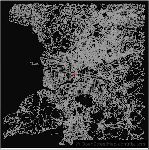
FIGURE 1. Map of 16 km radius around Kawajiri Station (the red dot in the center).

FIGURE 2

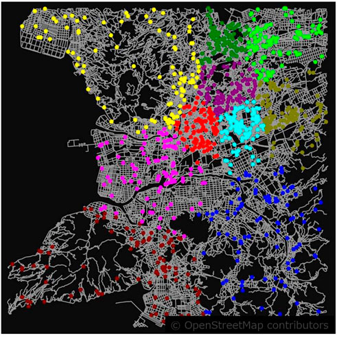
FIGURE 2. Ten instances with different geographic distributions in the base case.

TABLE 1

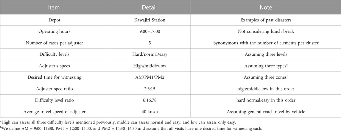
TABLE 1. Common settings for each instance.

TABLE 2

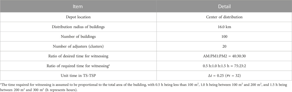
TABLE 2. Settings for each instance in the base case.

Furthermore, by setting up numerical experiments as described previously, H_div and H_matching in Eq. 13 can be written down specifically, respectively. Thus, the Hamiltonian $H_{\text{clustering}}^{\text{sim}}(\mathit{x})$ of the clustering phase in the numerical experiment is as follows:

$\begin{array}{cc}\hfill H_{\text{clustering}}^{\text{sim}}\left(\mathit{x}\right)& \hspace{0.17em}\hspace{0.17em}\hspace{0.17em}=A{\displaystyle \sum _{k=0}^{K-1}}{\displaystyle \sum _{\left(uv\right)\in E}}{D}_{uv}{x}_u^k{x}_v^k+B{\displaystyle \sum _{n=0}^{N-1}}{\left(1-{\displaystyle \sum _{k=0}^{K-1}}{x}_n^k\right)}^2+D{\displaystyle \sum _{k=0}^{K-1}}{\left(M-{\displaystyle \sum _{n=0}^{N-1}}{x}_n^k\right)}^2\hfill \\ \hfill & +C{\displaystyle \sum _{k=0}^{K-1}}\left\{{\left({\displaystyle \sum _{n\in \text{AM}}}{e}_n{x}_n^k\right)}^2+{\left({\displaystyle \sum _{n\in \text{PM}1}}{e}_n{x}_n^k\right)}^2+{\left({\displaystyle \sum _{n\in \text{PM}2}}{e}_n{x}_n^k\right)}^2\right\}\hfill \\ \hfill & +E\left\{{\displaystyle \sum _{n\in \text{Hard}}}{\left({\displaystyle \sum _{k\in \text{High}}}{x}_n^k-1\right)}^2+{\displaystyle \sum _{n\in \text{Normal}}}{\left({\displaystyle \sum _{k\in \text{High}\cup \text{Middle}}}{x}_n^k-1\right)}^2\right\},\hfill \end{array}(21)$

where N = 100, K = 20, and M = 5 correspond to the total number of visits, the total number of clusters, and the number of elements per cluster, respectively, and D_μν represent the distance matrix between visits μ and ν. We used A = 1, B = D = E = max(D_uv) × K × 2, C = 60 for each coefficient.

Similarly, the desired time constraint in Eq. 20 can be specifically written down, and the Hamiltonian $H_{\text{route}}^{\text{sim}}(\mathit{x})$ for the routing phase in the numerical experiment becomes

$\begin{array}{cc}\hfill H_{\text{route}}^{\text{sim}}\left(\mathit{x}\right)& ={\displaystyle \sum _{\begin{array}{c}1⩽a\ne b⩽N\\ 1⩽\tau ⩽T-1\end{array}}}\left(\frac{n_{ab}-\mu }{\rho }\times x_{\tau +e_{ab},a}{x}_{\tau ,b}+\lambda {\displaystyle \sum _{1⩽\delta \tau ⩽e_{ab}-1}}{x}_{\tau +\delta \tau ,a}{x}_{\tau ,b}\right)\hfill \\ \hfill & +\lambda \left({\displaystyle \sum _{\begin{array}{c}1⩽a<b⩽N\\ 1⩽\tau ⩽T\end{array}}}{x}_{\tau ,a}{x}_{\tau ,b}+{\displaystyle \sum _{\begin{array}{c}1⩽a⩽N\\ 1⩽\tau \ne {\tau }^{\prime }⩽T\end{array}}}{x}_{\tau ,a}{x}_{{\tau }^{\prime },a}\right)\hfill \\ \hfill & +\lambda \left({\displaystyle \sum _{\begin{array}{c}1⩽a⩽N\\ 1<\tau ⩽e_{a,\mathrm{d}\mathrm{e}\mathrm{p}\mathrm{o}\mathrm{t}}-1\end{array}}}{x}_{\tau ,a}\right)+\lambda \left({\displaystyle \sum _{\begin{array}{c}1⩽a⩽N\\ T-e_{\text{depot},a}⩽\tau ⩽T\end{array}}}{x}_{\tau ,a}\right)\hfill \\ \hfill & +\lambda \left\{{\displaystyle \sum _{a\in \text{AM}}}{\left({\displaystyle \sum _{\tau \in \text{AM}}}{x}_{\tau ,a}-1\right)}^2+{\displaystyle \sum _{b\in \text{PM}1}}{\left({\displaystyle \sum _{\tau \in \text{PM}1}}{x}_{\tau ,b}-1\right)}^2+{\displaystyle \sum _{c\in \text{PM}2}}{\left({\displaystyle \sum _{\tau \in \text{PM}2}}{x}_{\tau ,c}-1\right)}^2\right\},\hfill \end{array}(22)$

where N = 5 and T = 32⁴ correspond to the number of buildings per cluster and the number of time intervals, respectively, and ∑_a∈AM means taking the sum for building a such that the desired time for witnessing is the AM zone (the same for PM1 and PM2). n_ab in the first term can be obtained using the distance matrix D_ab and Eq. 15. We took λ = 40 for the coefficient.

3.2 Clustering

Here are some of the clustering results for each instance in the base case using the Hamiltonian in Eq. 21, accounting for the matchings of adjusters and buildings and dispersion in the required and desired time for witnessing.

Figure 3 shows⁵ a portion of the clustering results for instance No. 1 of the base case. The red point cloud in Figure 2, an example of an urban area, color-coded by clusters to visualize the location relationships and the data for each of the same clusters, is shown in Table 3. The distances between buildings in the cluster are short because of the high density near the depot, but the buildings closest to each other are necessarily not in the same cluster, which means the difficulty and spec correspondence and dispersion of desired and required time for witnessing are considered. For clusters other than those shown in Figure 3 and Table 3, the matching conditions for adjusters (clusters) and buildings were satisfied, and the required time and desired time for witnessing were appropriately distributed. There was no solution that did not satisfy the constraints (we call such a solution “break solution”) for either the SA or HSS solutions. No break solution occurred in all other instances, including sparsely populated areas, confirming that a feasible solution was obtained during the entire clustering phase.

FIGURE 3

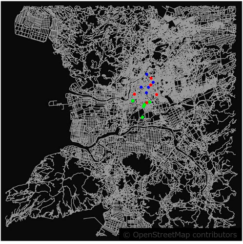
FIGURE 3. Location of the three clusters in instance No. 1 of the base case.

TABLE 3

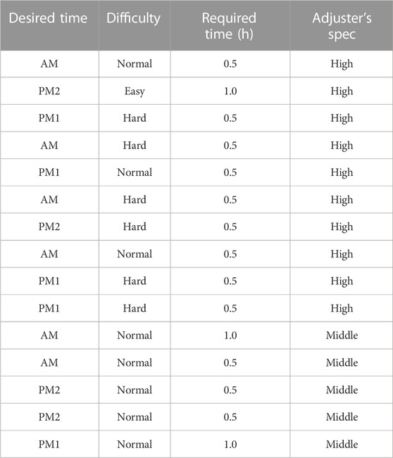
TABLE 3. Data for each of the three clusters in instance No. 1 of the base case: the top five, middle five, and bottom five points belong to different clusters (corresponding to red, blue, and green in Figure 3).

3.3 Routing

Here are some of the results of route optimization using Eq. 22 for the results of the clustering described in Section 3.2. In the routing phase, unlike the clustering phase, some cases occurred where feasible solutions were not obtained, so we also addressed such solutions.

Figure 4 visualizes the solution of route optimization for one cluster belonging to instance No. 1, corresponding to the top five clusters in Tables 3, 4 summarizes the travel time in the travel order for each visit. As shown in the chart, the route departs from the depot and returns to the depot within 8 h and is such that the desired time for witnessing each visit is satisfied. In addition, it was confirmed that all the route optimization solutions for the other clusters in instance No. 1 are also feasible.

FIGURE 4

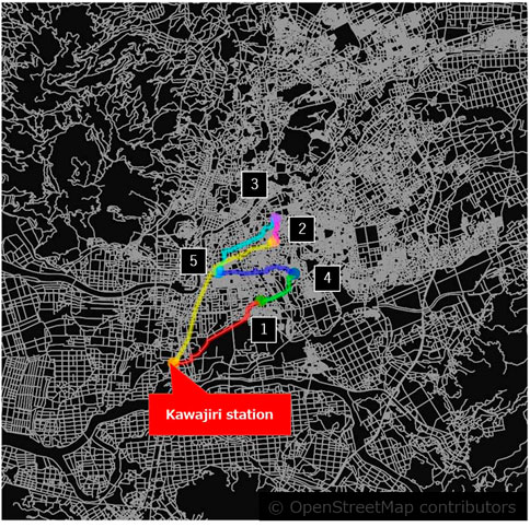
FIGURE 4. Route visualization for cluster No. 1 in instance No. 1 of the base case (paths are represented by red, green, blue, light blue, purple, and yellow in that order).

TABLE 4

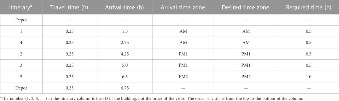
TABLE 4. Route optimization results for cluster No. 1 at instance No. 1 in the base case.

Conversely, only in instance No. 9, the brown point cloud in Figure 2, break solutions occurred in 2 out of 20 clusters. Figure 5 visualizes one of the clusters in instance No. 9, which is one of the solutions for which the constraint was broken. Table 5 summarizes the travel time for each building in order of travel; the desired time zone for witnessing the fourth visit is AM, but as a solution, it arrives at PM1, which breaks the desired time constraint. Similarly, for the other break solution, the break of the desired time constraint occurred in a cluster in a sparsely populated area far from the depot, resulting in a solution with a relatively long total travel distance. For these solutions, optimization with only the constraint term after excluding the cost term, the first term in Eq. 22, did not break, suggesting that the trade-off between travel time minimization and desired time constraints is more pronounced in the case of long total travel distances.

FIGURE 5

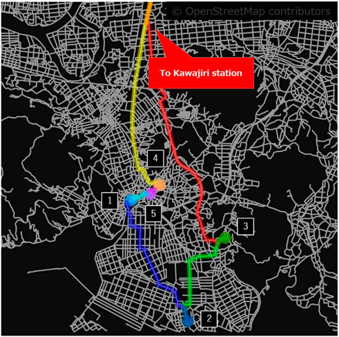
FIGURE 5. Route visualization for the break solution in instance No. 9 of the base case (paths are represented by red, green, blue, light blue, purple, and yellow in that order).

TABLE 5

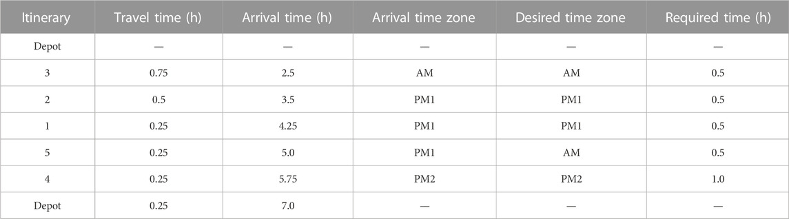
TABLE 5. Example of break solutions for route optimization results at instance No. 9 in the base case. The meaning of the “Itinerary” column is the same as in Table 4. A fourth visit breaks the desired time constraint.

3.4 Processing time

In the base case, we measured processing times in the two phases of the numerical experiment, the clustering and routing phases, and compared the differences between the solvers. The processing time was defined as the QUBO computation and solving time for both clustering and routing, both for one instance (for clustering, the process of dividing 100 buildings into 20 clusters of 5 elements each; for routing, the routing process for 20 clusters). The results are shown in Table 6. The processing time variation in clustering is small for HSS but large for routing. HSS, including quantum annealing, is superior in clustering, whereas SA is superior in the routing phase. The reason for these differences is that HSS performs quantum annealing while dividing QUBO according to the problem size, which is effective for large problems. However, extra processing time is presumably required for too small problems. The advantages of HSS will become even more effective when the problem size per processing unit increases during the routing phase.

TABLE 6

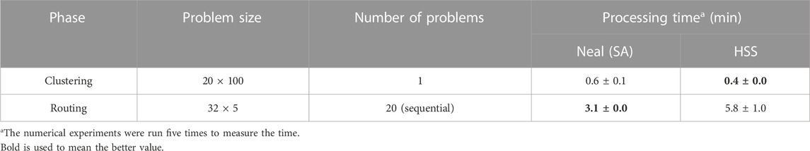
TABLE 6. Processing time for each solver in each phase.

For the break solution in the routing described previously, no feasible solution was obtained by HSS instead of SA. The break solution occurred even when the entire routing phase was solved with HSS from the beginning, and the same was true when both clustering and routing phases were solved consistently with HSS. Focusing especially on the clustering phase, where the superiority of the HSS solution was confirmed in terms of processing time, the percentage of solutions with the smaller energy value is shown in Table 7. The largest energy difference occurred at instance No. 6, yellow dots in Figure 2, where the HSS solution was 4.6% smaller than the SA solution in terms of magnitude. However, this level of energy difference is considered to have a small impact on the routing phase solution because there are cases where the break solution occurs in the routing phase, regardless of whether the HSS or SA solution is used in the clustering phase.

TABLE 7

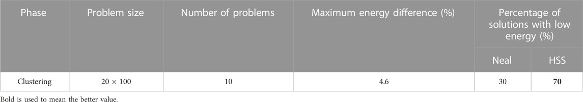
TABLE 7. Energetic advantage of each solver in the clustering phase.

In this paper, clustering is performed in the form of assigning a building to each adjuster, so even if a feasible solution is obtained in the clustering phase, the impact of the solution will strongly affect the next routing phase. To reduce this effect, for example, let us consider the case where the number of elements in one cluster increased. In this form of TS-VRP, a route optimization in which several people visit dozens of buildings, it may be possible to reduce the number of break solutions in the HSS solver and reduce the processing time. Mitigating the constraints that the solution of the clustering phase imposes on the next routing phase is a topic for future work.

3.5 Results of other cases

A list of changes from the base case for each case is shown in Table 8. The application of the results of five numerical experiments, each with SA for all cases, is shown in Table 9. Here, the processing time is calculated by the total processing time of the clustering and routing phases according to Table 6. The percentage of break solutions means the percentage of the total 200 route optimization solutions. In all cases, the changes in each setting value affected the processing time and solution quality. However, especially for case #4, although the processing time was reduced, the quality dropped significantly due to many broken solutions in the final routing phase caused by the increase in unit time in route optimization. There are instances of urban and sparsely populated areas in the numerical experiments. Particularly, in the former, where buildings to visit are relatively close to each other, a too large unit time would have a negative impact on the routing optimization. Therefore, an appropriate value for the problem setting should be set like the unit time of route optimization. It was also found that when there is no significant bias in the desired time zone, as in #1 and #2, a feasible solution is sufficient in the area within a radius of 16 km. For cases such as #5–#7, where there is a significant bias in the desired time zone, the Q2Q approach requires measures to ease the constraints on the routing solution by adjusting the size of the solution passed between the two phases, as described in Section 3.4. As also discussed in Section 3.4, the HSS has advantages, at least in clustering. Therefore, when HSS is used for severe cases such as #2, #7, and #8, it may be possible to suppress break solutions.

TABLE 8

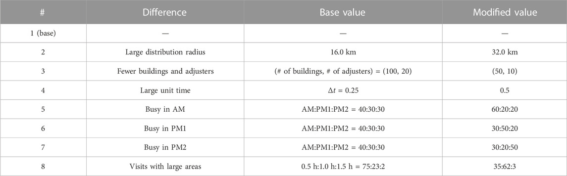
TABLE 8. Differences between the base case and other cases.

TABLE 9

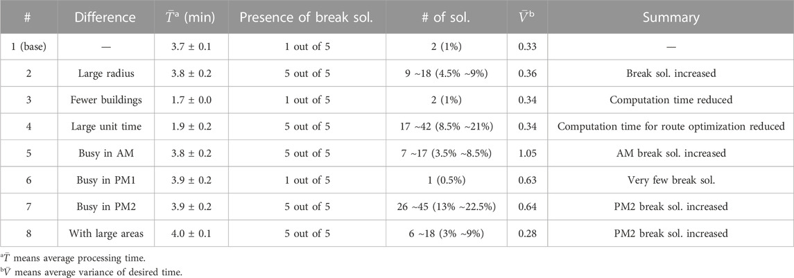
TABLE 9. Summary of numerical experimental results in each case.

Conversely, it is also important in real-world problems to consider multiple targets for optimization. In this paper, we aimed to optimize total travel time and total witnessing time, but various optimization targets depend on the needs, such as optimization to minimize the number of adjusters to be dispatched or optimization to complete all witnessing in a minimum number of operating days at the expense of operating time. These will be discussed in future prospects.

4 Conclusion

We formulate a real-world problem, the adjuster route optimization problem (ARP) in a QUBO form, and propose a method to solve it using quantum annealing. ARP is an optimization problem that extends VRP and can be solved using a 2-phase-heuristics approach, as in [23]. In the clustering phase, to determine the buildings to be witnessed by the adjuster, constraints were introduced to achieve adjuster/building matching and distribute the required and desired time for witnessing without bias for the next routing phase. In the routing phase, to determine the order of witnessing by the adjuster, the constraint was introduced to satisfy the desired time for witnessing that each building has. These constraints may be applicable not only to ARP but also to other real-world problems related to VRP.

Furthermore, we confirmed that our formulation works correctly by conducting numerical experiments using the actual quantum annealing machine D-Wave. We also confirmed the superiority of D-Wave Leap’s Hybrid Solver Service over classical algorithms. We hope that our research will help speed up witnessing operations during disasters using quantum computers.

While the constraints introduced in this paper alone are sufficient to make the model practical, additional conditions will likely need to be considered to actually implement the model in witnessing operations. For example, it may be necessary to consider break times, such as lunch (this can be realized by “state” in [32]), or routes that cannot be taken in the event of a disaster in the distance matrix. It is also a challenge to add and validate constraints to the model that may be necessary in the future.

Data availability statement

The original contributions presented in the study are included in the article/supplementary material. Further inquiries can be directed to the corresponding author.

Author contributions

NM mainly contributed to the construction and verification of the clustering Hamiltonian and performed all the numerical experiments through the clustering and routing phases. SF mainly contributed to routing Hamiltonian, especially the constraint term newly introduced, and conducted the numerical experiment of routing for verification. All authors contributed to the article and approved the submitted version.

Acknowledgments

The authors would like to thank Jun Mino for helpful discussions about ARP. The authors also want to thank the member of the Digital Promotion Department at Cognivision Inc., especially Masakazu Sato, Kazutaka Murakami, and Mitsuaki Nozawa for the careful reading of the article and the suggestions for improvements.

Conflict of interest

NM and SF were employed by Cognivision Inc.

Publisher’s note

All claims expressed in this article are solely those of the authors and do not necessarily represent those of their affiliated organizations, or those of the publisher, the editors, and the reviewers. Any product that may be evaluated in this article, or claim that may be made by its manufacturer, is not guaranteed or endorsed by the publisher.

Footnotes

¹Non-deterministic polynomial time.

²Equation 4 contains only the leading-order term. More rigorous discussion is given by Kimura and Nishimori [34].

³https://docs.ocean.dwavesys.com/en/stable/.

⁴As the total operating hours is 8 h (Table 1) and the unit time is Δt = 0.25 (Table 2), the number of time intervals is 8/0.25 = 32, according to the correspondence Eq. 14.

⁵For ease of viewing, the figure shows only three of the 20 clusters contained in each instance.

References

1. Karp RM. Reducibility among combinatorial problems. Complexity Comput Computations (1972) 85:85–103. doi:10.1007/978-1-4684-2001-2_9

CrossRef Full Text | Google Scholar

2. Kadowaki T, Nishimori H. Quantum annealing in the transverse Ising model. Phys Rev E (1998) 58:5355–63. doi:10.1103/PhysRevE.58.5355

CrossRef Full Text | Google Scholar

3. Johnson MW, Amin MHS, Gildert S, Lanting T, Hamze F, Dickson N, et al. Quantum annealing with manufactured spins. Nature (2011) 473:194–8. doi:10.1038/nature10012

PubMed Abstract | CrossRef Full Text | Google Scholar

4. Venturelli D, Marchand DJJ, Rojo G. Quantum annealing implementation of job-shop scheduling. COPLAS (2016). doi:10.48550/arXiv.1506.08479

CrossRef Full Text | Google Scholar

5. Ikeda K, Nakamura Y, Humble TS. Application of quantum annealing to nurse scheduling problem. Scientific Rep (2019) 9:12837. doi:10.1038/s41598-019-49172-3

CrossRef Full Text | Google Scholar

6. Venturelli D, Kondratyev A. Reverse quantum annealing approach to portfolio optimization problems. Quan Machine Intelligence (2019) 1:17–30. doi:10.1007/s42484-019-00001-w

CrossRef Full Text | Google Scholar

7. Neven H, Denchev VS, Rose G, Macready WG. QBoost: Large scale classifier training with adiabatic quantum optimization. JMLR: Workshop Conf Proc (2012) 25:333–48.

Google Scholar

8. O’Malley D, Vesselinov VV, Alexandrov BS, Alexandrov L. Nonnegative/binary matrix factorization with a D-Wave quantum annealer (2017). arXiv:1704.01605. doi:10.1371/journal.pone.0206653

CrossRef Full Text | Google Scholar

9. von Dollen D, Neukart F, Weimer D, Bäck T. Quantum-assisted feature selection for vehicle price prediction modeling (2021). arXiv:2104.04049. doi:10.48550/arXiv.2104.04049

CrossRef Full Text | Google Scholar

10. Benkner MS, Golyanik V, Theobalt C, Moeller M. Adiabatic quantum graph matching with permutation matrix constraints. In: 2020 International Conference on 3D Vision (3DV). Fukuoka, Japan: IEEE (2020). doi:10.1109/3DV50981.2020.00068

CrossRef Full Text | Google Scholar

11. Birdal T, Golyanik V, Theobalt C, Guibas L. Quantum permutation synchronization. In: 2021 IEEE/CVF Conference on Computer Vision and Pattern Recognition (CVPR). Nashville, TN, USA: IEEE (2021). doi:10.1109/CVPR46437.2021.01292

CrossRef Full Text | Google Scholar

12. Xia R, Bian T, Kais S. Electronic structure calculations and the Ising Hamiltonian. The J Phys Chem B (2017) 122:3384–95. doi:10.1021/acs.jpcb.7b10371

PubMed Abstract | CrossRef Full Text | Google Scholar

13. Streif M, Neukart F, Leib M. Solving quantum chemistry problems with a D-wave quantum annealer: First international workshop, QTOP 2019, Munich, Germany, March 18, 2019, proceedings. In: Quantum Technology and optimization problems (2017). p. 111–22. doi:10.1007/978-3-030-14082-3_10

CrossRef Full Text | Google Scholar

14. Ohzeki M, Miki A, Miyama MJ, Terabe M. Control of automated guided vehicles without collision by quantum annealer and digital devices. Front Comput Sci (2019) 1. doi:10.3389/fcomp.2019.00009

CrossRef Full Text | Google Scholar

15. Neukart F, Compostella G, Seidel C, von Dollen D, Yarkoni S, Parney B. Traffic flow optimization using a quantum annealer. Front ICT (2017) 4. doi:10.3389/fict.2017.00029

CrossRef Full Text | Google Scholar

16. Nishimura N, Tanahashi K, Suganuma K, Miyama MJ, Ohzeki M. Item listing optimization for E-commerce websites based on diversity. Front Comput Sci (2019) 1. doi:10.3389/fcomp.2019.00002

CrossRef Full Text | Google Scholar

17. Dantzig GB, Ramser JH. The truck dispatching problem. Manage Sci (1959) 6:80–91. doi:10.1287/mnsc.6.1.80

CrossRef Full Text | Google Scholar

18. Braysy O, Gendreau M. Vehicle routing problem with time windows, part I: Route construction and local search algorithms. Transportation Sci (2005) 39:104–18. doi:10.1287/trsc.1030.0056

CrossRef Full Text | Google Scholar

19. de Oliveira HCB, Vasconcelos GC. A hybrid search method for the vehicle routing problem with time windows. Ann Operations Res (2010) 180:125–44. doi:10.1007/s10479-008-0487-y

CrossRef Full Text | Google Scholar

20. Ralphs TK, Kopman L, Pulleyblank WR, Trotter LE. On the capacitated vehicle routing problem. Math Programming (2003) 94:343–59. doi:10.1007/s10107-002-0323-0

CrossRef Full Text | Google Scholar

21. Boothby K, Bunyk P, Raymond J, Roy A. Next-generation topology of D-Wave quantum processors (2020). arXiv:2003.00133. doi:10.48550/arXiv.2003.00133

CrossRef Full Text | Google Scholar

22. Laporte G, Semet F. Classical heuristics for the capacitated VRP. In: The vehicle routing problem. Philadelphia, Pennsylvania, USA: Society for Industrial and Applied Mathematics (2002). chap. 5.

Google Scholar

23. Feld S, Roch C, Gabor T, Seidel C, Neukart F, Galter I, et al. A hybrid solution method for the capacitated vehicle routing problem using a quantum annealer. Front ICT (2019) 6:1–13. doi:10.3389/fict.2019.00013

CrossRef Full Text | Google Scholar

24. Laporte G. The traveling salesman problem: An overview of exact and approximate algorithms. Eur J Oper Res (1992) 59:231–47. doi:10.1016/0377-2217(92)90138-Y

CrossRef Full Text | Google Scholar

25. Tsukamoto S, Takatsu M, Matsubara S, Tamura H. An accelerator architecture for combinatorial optimization problems. Fujitsu Sci (2017) 53.

Google Scholar

26. Yoshimura C, Yamaoka M, Aoki H, Mizuno H. Spatial computing architecture using randomness of memory cell stability under voltage control. In: 2013 European Conference on Circuit Theory and Design (ECCTD). Dresden, Germany: IEEE (2013). doi:10.1109/ECCTD.2013.6662276

CrossRef Full Text | Google Scholar

27. Yarkoni S, Raponi E, Bäck T, Schmitt S. Quantum annealing for industry applications: Introduction and review. Rep Prog Phys (2022) 85:104001. doi:10.1088/1361-6633/ac8c54

CrossRef Full Text | Google Scholar

28. Lucas A. Ising formulations of many NP problems. Front Phys (2014) 2. doi:10.3389/fphy.2014.00005

CrossRef Full Text | Google Scholar

29. Yonaga K, Miyama MJ, Ohzeki M. Solving inequality-constrained binary optimization problems on quantum annealer (2020). arXiv:2012.06119. doi:10.48550/arXiv.2012.06119

CrossRef Full Text | Google Scholar

30. Dash S, Günlük O, Lodi A, Tramontani A. A time bucket formulation for the traveling salesman problem with time windows. Informs J Comput (2010) 24:132–47. doi:10.1287/ijoc.1100.0432

CrossRef Full Text | Google Scholar

31. Kara I, Derya T. Formulations for minimizing tour duration of the traveling salesman problem with time windows. Proced Econ Finance (2015) 26:1026–34. doi:10.1016/S2212-5671(15)00926-0

CrossRef Full Text | Google Scholar

32. Irie H, Wongpaisarnsin G, Terabe M, Miki A, Taguchi S. Quantum annealing of vehicle routing problem with time, state and capacity. In: S Feld, and C Linnhoff-Popien, editors. Quantum Technology and optimization problems. QTOP 2019. Lecture notes in computer science. Cham: Springer (2019). p. 145–56. doi:10.1007/978-3-030-14082-3_13

CrossRef Full Text | Google Scholar

33. Kirkpatrick S, Gelatt CD, Vecchi MP. Optimization by simulated annealing. Science (1986) 220:671–80. doi:10.1126/science.220.4598.671

CrossRef Full Text | Google Scholar

34. Kimura Y, Nishimori H. Rigorous convergence condition for quantum annealing. J Phys A: Math Theor (2022) 55:435302. doi:10.1088/1751-8121/ac9dce

CrossRef Full Text | Google Scholar