Recirculation of plasmasphere material during idealized magnetic storms

1 Introduction

The plasmasphere is a cold ($\sim 1$ eV) dense (10³–10⁴/cm³) region of plasma which corotates with Earth [1]. During extended periods of low activity in the solar wind, the plasmasphere fills up to a saturation density as it reaches a diffusive equilibrium with the ionosphere. During periods of high activity, enhanced dayside reconnection with the Interplanetary Magnetic Field (IMF) causes mass-loaded magnetic flux tubes in the plasmasphere to be advected out to the reconnection region as described by the Dungey cycle [2] during southward interplanetary magnetic field. As the process of magnetic reconnection continues along the dayside magnetopause, a plume of plasmasphere material forms on the dayside. This plume drains plasma from the plasmasphere along the path of the advecting flux tubes. The plasma remains trapped on the field line through the process of reconnection and remains with the field line as it continues through the Dungey cycle. Su et al. 2001, found evidence of plasmasphere material on open field lines with magnetosheath material during periods of K_p ≥ 4 using both the Interball Auroral Probe and Polar satellites [3]. Su did not find as many instances of plasmasphere material on open field lines as they thought they would and among other causes, speculated that plasmaspheric material heating could make it indistinguishable from magnetosheath plasma using their method. Walsh et al. 2014, when studying the impact of the plasmasphere plume on the dayside reconnection rate, found that the cold plume plasma possessed energy around 10 eV enhancing the energy flux at that band as THEMIS D crossed from the magnetosheath into the magnetosphere [4]. After reconnection the field line is no longer closed with both ends on Earth, but is rather an open field line, with one end anchored to Earth and the other connected to the Interplanetary Magnetic Field (IMF). The question at this point is if the velocity of the trapped plasma along the field line is large enough that a significant fraction of it is within the loss cone, to be lost to scattering in the ionosphere, or travel further into the IMF before being trapped by reconnection on the night side. The plasma could recirculate through one of two paths. The first is that the plasma can be transported through the lobes by the advecting magnetic flux tubes and become trapped on closed field lines due to magnetic reconnection on the night side. Alternatively the plasma could recirculate by traveling along the flanks and mixing with the plasma sheet material in the tail through viscous interactions.

The recirculation of the plasmasphere was first proposed by Freeman et al. (1977) [5]. That paper proposed that the plasmaspheric material may either recirculate over the poles and-or around the flanks. Borovsky et al. (1997) [6] estimates that the plasmasphere can provide up to twice the needed material to explain the super dense plasma sheet. A six-step process was proposed by which the plasmaspheric material can recirculate over the poles. Using satellite data from four LANL-MPA instruments, it was demonstrated that plasmaspheric material does undergo the first three steps of the proposed six-step process. However, due to the orbits of the LANL satellites being used it was not possible to demonstrate conclusively that the plasmaspheric material went any further then step three of the six. Borovsky notes that the conditions necessary for the six-step process would also allow the penetration of solar wind into the plasma sheet, making it difficult to determine if observed material in the tail is of plasmasphere or solar wind origin. Daglis et al. (1999) demonstrated ring current ions primarily come from the plasma sheet and the solar wind. However, the plasma sheet is itself fed by the high latitude ionosphere and the solar wind. Thus, the ultimate source of ring current particles is the high latitude ionosphere and solar wind [7]. Su et al. (2001) demonstrated that plasmasphere material could be located on high-latitude open field lines in some cases, finding it twice in a sampling of 21 events using the Interball Auroral Probe and four times over 8 months using Polar [3].

Simulations and models have also been used to investigate this issue. In Elphic et al. (1997) [8], Elphic used the Weber 1996 and Tsyganenko 1989 models to track magnetic flux tubes by following their foot points in the ionosphere [9, 10]. Elphic found that in storm conditions the magnetic field flux tubes representing plasmasphere flux tubes did recirculate over the poles and not around the flank as was thought possible by Freeman. This study was limited as it did not include the recursive effects of the plasma being transported and included only one simulated event. Moore et al. (2008) [11] used the Lyon-Fedder-Mobarry (LFM) model to trace test particles that were given initial velocities and energies representative of the plasmasphere by the coupled Comprehensive Ring Current Model (CRCM). The contribution to the ring current of test particles that recirculated back into the region of the CRCM was then compared to the contribution to the ring current from other populations. It was found that the plasmasphere contributed about the same to the ring current as the polar wind, though its contribution lagged by about an hour, and that the plasmasphere contributed less then the solar and auroral wind sources. The Moore et al. (2008) study was limited by a lack of self-consistency. The plasmaspheric particles in the LFM portion were test particles, and the ionosphere particles in the CRCM portion were not coupling to the LFM model. It was suggested that treating the plasmasphere particles self-consistently and including the ionosphere particles in the LFM/CRCM coupling could substantially change the results.

Using observations to resolve the issue is difficult due to the composition of the plasma from the solar wind, plasmasphere, and ionosphere, which are all dominated by hydrogen as well as the large-scale nature of the problem. Until recently, simulations have not been up to the task of tracking multiple populations of ions in the magnetosphere on a global scale, due both to a lack of computational power and the outer boundary of dedicated plasmaspheric codes typically being placed at 8–10 R_E, which is to close to Earth to capture recirculation of the plasma [11–13]. However, recent advancements both in modeling approaches and computing power have made it possible to study the fate of plasmaspheric material on a global scale in numerical simulations.

This study presents two simulations using the Space Weather Modeling Framework in a novel configuration to study the fate of plasmaspheric material during magnetic storms. The simulations approach the recursive relationship of the inner magnetosphere and solar wind coupling from a self-consistent manner. This capability will enable us to address the fate of the plasmasphere once it enters to solar wind, and begin to resolve the outstanding question.

2 Methodology

2.1 Configuration of the SWMF

It is difficult to design a single model which captures the intricacies of the near-Earth space environment due to the large range in spatial and temporal scales, plasma composition, and complicated physics this entails. The Space Weather Modeling Framework [14] approaches this challenge by coupling together otherwise separate models which are specialized to capture the dynamics of sub regions, or particular processes of space weather. This coupling typically includes passing information about key values, such as the density and temperature of a plasma, between models to ensure that model solutions are similar both temporally and spatially. For this study the SWMF is configured to couple three models: the Block-Adaptive-Tree-Solarwind-Roe-Up-Wind-Scheme (BATS-R-US), the Dynamic Global Core Plasma Model (DGCPM) and the Ridley Ionosphere Model (RIM). BATS-R-US is a multi-fluid multi-species global magnetohydrodynamic (MHD) code [15]. In our case the simulation is configured with two fluids, both hydrogen. The first fluid is defined to be the known sources of the ring current, namely the solar wind and the high latitude ionospheric outflow [16, 17]. For the sake of simplicity we refer to the high latitude ionospheric outflow as the polar wind through out the rest of the report. The second BATS-R-US fluid represents the cold plasmasphere population and is coupled to DGCPM. For each fluid BATS-R-US solves the magnetohydrodynamic equations.

DGCPM is a two dimensional plasmasphere code which solves for flux tube ion content on the ionosphere grid, projected into the equatorial plane [18]. DGCPM is configured within the Space Weather Modeling Framework to have one way coupling with BATS-R-US. Within 10 R_E of Earth BATS-R-US will nudge its solution for the mass density of the plasmasphere fluid towards that of DGCPM, such that the solutions converge rapidly [15, 19]. BATS-R-US is coupled to RIM in a two-way manner. BATS-R-US provides field aligned currents to RIM which in turn provides the E × B values at the inner boundary of BATS-R-US to set the velocity of all fluids there [20]. RIM and DGCPM are one-way coupled. DGCPM uses the solution of the electric potential generated by RIM to calculate the electric field in the equatorial plane [18]. For a graphical representation of this configuration refer to Figure 1.

FIGURE 1

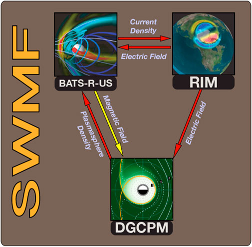
FIGURE 1. Configuration of the SWMF and coupling between sub modules. Red arrows depict coupling in the SWMF model which currently exists. The yellow arrow depicts coupling to be added to the future, to be discussed later.

Figure 1 summarizes the coupling of BATS-R-US, DGCPM and RIM through the framework of the SWMF. The red arrows in Figure 1 represent the coupling described above that was used in this study. The yellow arrow labeled “Magnetic Field” pointing from BATS-R-US to DGCPM indicates a desired future coupling to be discussed in future work.

Several simplifying assumptions were made in the BATS-R-US simulation. The first assumption is that Earth’s magnetic field can be represented as a dipole. The second assumption is that Earth’s magnetic dipole is parallel to Earth’s axis of rotation. The final assumption is that the axis of rotation is perpendicular to the ecliptic plane. DGCPM assumes a dipole with the same configuration, and thus by using a similar magnetic field configuration in BATS-R-US we minimize the effects of having non-coupled magnetic fields between the two models. The consequence of not having this coupling this will be discussed later.

The novel part of this configuration of the SWMF is that, on closed field lines within 10 R_E, the dynamics of the plasmasphere fluid in BATS-R-US are dictated by DGCPM. The DGCPM code has been shown to provide an accurate description of the plasmapause, as long as the ionospheric potential model is itself an accurate representation [18]. In this study we are using the SWMF to provide the ionospheric potential, via coupling to RIM, to drive DGCPM. This configuration has all of the advantages of the best preforming model to drive DGCPM as identified by Ridley et al. 2014 [18]. Therefore this configuration should provide the most accurate simulation of plasmaspheric dynamics to date within the SWMF.

Figure 2 shows a comparison of the plasmasphere in different configurations of BATS-R-US and DGCPM running as sub components of the SWMF. In Figure 2A we see the plasmasphere as produced by BATS-R-US running in a stand alone single fluid configuration. Figure 2B is BATS-R-US in a multi-fluid stand alone configuration with a dedicated plasmaspheric fluid. The difference between the configuration for 2a and 2b is that the inner boundary condition for the plasmaspheric fluid was increased from 28 amu/cc, a value typical of the polar wind, to 500 amu/cc. This inner boundary generates a much denser pseudo-plasmasphere. However, even with the configuration of 2b the plasmasphere and its plume is still very diffuse, lacking a sharply defined plasmapause. Figure 2C is a standalone DGCPM simulation, while Figure 2D is multi-fluid BATS-R-US coupled to DGCPM via the SWMF. As can be clearly seen in Figures 2A,B a global MHD code, even with a dedicated plasmasphere fluid, is a poor representation of the dynamics that a cold dense plasma undergoes near Earth. The standalone DGCPM simulation gives a very detailed plasmasphere (though some features, such as the tendrils visible near midnight, may not be real), but standalone DGCPM lacks the ability to include the effects of the solar wind, plasma sheet and anything beyond 10 R_E from Earth. While this gives us a detailed view of the plasmasphere, it limits our understanding of the entire system. Thus by coupling DGCPM to BATS-R-US, we capture the best of both worlds. We are able to see and model the solar wind and the broader near-Earth space environment while maintaining a detailed view of the plasmasphere. Importantly, this enables us to study in a self-consistent manner how plasmaspheric material evolves once it leaves the inner magnetosphere, and whether it is captured by night side reconnection and advected back towards Earth. Appendix A contains information on the input files and the full configuration for the SWMF as it appearers in this work.

FIGURE 2

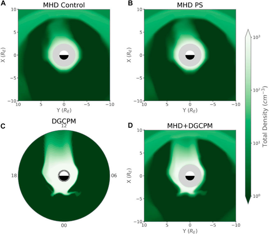
FIGURE 2. Coupling of BATS-R-US and DGCPM. (A) Z = 0 slice of single fluid BATS-R-US in standalone mode. GSE coordinates. (B) Z = 0 slice of two fluid BATS-R-US in standalone mode. GSE coordinates. (C) Standalone DGCPM out to 10 R_E. LT and Radius (D) Z = 0 SWMF coupling dual fluid BATS-R-US and DGCPM. GSE coordinates.

2.1.1 Configuration of BATS-R-US

BATS-R-US is a multi-fluid multi-species global MHD code. This type of code solves the magnetohydrodynamic equations for fluid packets, with each fluid able to be a separate species or represent a different population. In the configuration for the following simulations BATS-R-US is configured with two fluids, both of which are hydrogen. The first fluid is the combined solar wind and polar wind, while the second is a dedicated plasmasphere fluid. BATS-R-US handles the bulk of the computational space while the other models, DGCPM and RIM, handle specific components of the inner magnetosphere and ionosphere. BATS-R-US runs on a Cartesian grid in the GSM coordinate system. A key feature of BATS-R-US is the flexible grid size of cells within the region of computation. In the configuration used in this study, the entire inner magnetosphere was resolved to a resolution of 1/8 Earth Radii (R_E). The maximum grid size was cubes of 8 R_E a side, while the minimum was cubes of 1/16 R_E a side. The grid is set with areas of high resolution near the magnetosheath and Earth starting at 1/16 R_E cells and stepping down from there. Farther down the tail, the grid is dominated by cells of 8 R_E. For a more detailed discussion of the grid see Welling and Liemohn 2014 [21].

Within BATS-R-US, the upstream boundary condition is determined by solar wind and interplanetary magnetic field (IMF) values read from a file. Upstream plasma values must be provided for every fluid in the MHD simulation. This restriction is because the numerical schemes of BATS-R-US cannot handle zero densities or temperatures and must have all the fluids present in the whole computational domain. As such, low values are chosen for non-dominant ions such that their contribution to total density and energies are negligible in the region dominated by the solar wind. The inner boundary is determined by predefined values made to mimic the polar wind. In BATS-R-US, the inner boundary values for the combined solar and polar wind fluid were set to 28 amu/cc at 25,000.0 K. For the plasmasphere fluid, values of 0.01 amu/cc and 25,000 K were assigned. The low amu/cc count of the plasmasphere prevents the inner boundary condition from becoming a significant source of plasmasphere ions.

2.1.2 Configuration of DGCPM

DGCPM is a single species two-dimensional code solving for the flux tube content measured in electrons per Weber [22]. In the filling and emptying of dayside closed magnetic field lines, DGCPM works to drive each flux tube towards its saturation density. The saturation density is defined as the density at which dynamic equilibrium is reached between loss and filling processes on closed magnetic field lines. The saturation density was determined empirically by [23] as,

$n_{\mathit{sat}}=10^{\left(-0.3245L+3.9043\right)}(1)$

given in electrons per cubic centimeter where L is the L-shell of the field line in the equatorial plane. On the dayside, closed flux tubes whose density exceeds n_sat have their density reduced to the saturation value. If, however, the density on such a field line is less then n_sat, a refilling flux is applied up to a pre-defined maximum flux. On open field lines, night or day, the same decay rate is applied. A decay rate is also applied to closed field lines on the night side. Plasma convection is handled by a second-order upwind scheme with a Superbee limiter [18]. While at the core, DGCPM is the same model as from Ober et al. 1997, it has undergone significant modification to be fully integrated in the SWMF [12, 14, 24]. For a more detailed discussion on how DGCPM functions, see Ober et al. 1997 [12].

The temperature of the plasma is fixed to be 1 eV for the purpose of coupling to BATS-R-US. This value is consistent with values given in the literature which range from 0.1 eV to 2 eV [1, 25]. This temperature along with the density of the plasma in DGCPM is used to calculate the pressure of the plasmasphere in BATS-R-US. This pressure is always a small fraction (≤10%) of the total pressure of non-plasmaspheric fluid in BATS-R-US and does not significantly affect the MHD calculation. Therefore, the calculation is fairly insensitive to the choice made for the temperature of the plasmaspheric plasma during coupling. DGCPM assumes a dipole field and does not receive non-dipole values from BATS-R-US. BATS-R-US self-consistently calculates the magnetic field, though it also assumes a dipole for Earth’s magnetic field. The possible consequences of this discrepancy will be discussed in future work.

The initial condition of DGCPM for these runs is one of a dense plasmasphere at or near the saturation density. This initial condition is chosen specifically to give us the best chance at seeing recirculation occur. It is important to keep this in mind when we discuss the results as this may bias us to see recirculation as more of a dominant source relative to the solar and polar winds. However, as the fullness of the plasmasphere does not affect the likelihood of a geomagnetic storm occurring these results represent the recirculation of the plasmasphere when it is at or near saturation.

2.1.3 Configuration of RIM

The Ridley Ionosphere Model (RIM) is a 2D spherical electric potential solver. RIM uses the field aligned currents from BATS-R-US to calculate the electric potential as:

$J_R={\nabla }_{\perp }\left(\mathrm{\Sigma }\cdot {\nabla }_{\perp }\mathrm{\Phi }\right)(2)$

where J_R represents the radial currents supplied by BATS-R-US. S is the conductance tensor (comprising both Hall and Pedersen conductance), and Φ is the electric potential in the ionosphere [20]. The currents from BATS-R-US are taken at a fixed altitude near the inner boundary. The current values are then mapped along dipole field lines to the ionosphere. The gradient of the potential yields the electric field which can be combined with BATS-R-US’s magnetic field to yield the E × B value, which is returned to BATS-R-US. In BATS-R-US, the returned E × B values are used to set the tangential velocity of the plasma about the inner boundary. A major challenge for ionosphere models is getting a realistic conductance. Conductance is primarily derived from two sources: ionization due to extreme ultra-violet (EUV) radiation [26] and ionization due to precipitating ions and electrons [27–29]. Conductance caused by extreme ultra-violet radiation is included via an empirical formula, which is a function of solar zenith angle [20]. RIM uses an empirical model based on an Assimilate Mapping of Ionospheric Electrodynamics (AMIE) study to drive the conductance caused by particle precipitation [30]. The Assimilate Mapping of Ionospheric Electrodynamics study produced a simple relationship for the strength of field aligned currents and Hall or Pedersen conductance:

$\mathrm{\Sigma }={\mathrm{\Sigma }}_0{e}^{-A|J_{\Vert }|}(3)$

where Σ₀ and A are functions of latitude and longitude. Two sets of coefficients are used, one for upward, and one for downward field aligned currents. For a detailed discussion of how the model works see [19].

RIM is also coupled to DGCPM. In the one way coupling between DGCPM and RIM, DGCPM requests electric field data from RIM. RIM can calculate the electric potential down to the low latitudes and thus provide the electric field to the entire DGCPM domain.

3 Analysis

3.1 Ideal square wave

The first simulation presented for this study is an Ideal Square Wave event. The solar wind has a constant density and velocity of 5/cm⁻³ and 450 km/s. The B_z component of the interplanetary magnetic field (IMF) begins at +5 nT flipping to -10 nT after 8 h, marking the start of the storm. There is a constant value of B_y = +2 nT which moves the reconnection line slightly out of the equatorial plane. The B_x component of the solar wind is zero throughout the simulation. Such ideal event conditions are chosen to demonstrate that the recirculation of plasmaspheric plasma is possible. The long period of quiet time preceding the start of the storm allows the simulation to build a dense and saturated plasmasphere. The sudden southward turning and constant negative B_z provides the maximum amount of time for plasmaspheric material to recirculate. Having an extended southward B_z period increases the chances that we see such an affect occur. In addition, the constant negative B_z drives reconnection on the dayside, which in turn drives the formation of the dayside plasma plume. Relatively typical solar wind velocity and density were chosen to demonstrate that our results are not a consequence of rare or unusual solar wind conditions.

Figures 3A–F shows the state of the plasmasphere in BATS-R-US at three key points in the simulation. Figures 3A–C shows 2D slices from the Y = 0 plane, while Figures 3D–F shows 2D slices of the Z = 0 plane. The black and white circle at the origin of each plot represents the Earth. The white half of the circle represents the dayside and the black half the night side of Earth. The light gray circle around the Earth represents the inner boundary of BATS-R-US. The color map of each plot is the density of the plasmaspheric fluid in BATS-R-US at that point in the domain. The yellow arrows represent the magnitude and direction of the velocity vector field for the plasmaspheric fluid. The velocity arrows in the upstream solar wind of each plot are 450 km/s. In subplots A-C in Figure 3, the black contours are closed magnetic field lines, meaning both foot points of the field line are in the ionosphere. The red contour represents the last closed magnetic field line, whereas the white contours represent open field lines. Each column contains slices from a single time in the simulation. The times chosen are 08 Hr 40 Min, 09 Hr 19 Min, and 09 Hr 52 Min, for the left, center, and right columns respectively. Recall that the storm began with a southward turning of B_z at 8 Hr. Thus, the times shown in Figure 3 are from 40 Min, 1 Hr 19 Min, and 1 Hr 52 Min after the storm began respectively. These times show three key moments of plasmasphere recirculation. In Figure 3D, the dayside plume encounters the dayside reconnection line and begins venting plasmaspheric plasma along the dawn flank. This feature is highlighted by the red box in Figure 3D. We see in Figure 3A that the dayside lobes do not contain much plasmaspheric material. There is a strong divergence in the flow pattern on the night side in Figure 3B corresponding to the location of night side reconnection, marked by a red box. We also see that the lobes are beginning to fill, indicating that at this time, plasmaspheric material has not recirculated over the poles. In Figure 3E, we see a good deal of plasma has continued to leak out of the dayside plume and has begun to fill the plasma sheet with recirculated material. This process is aided by the flank biased plume which, when comparing to Figures 3C, 3F, is venting much more material along the flanks then though the dayside lobes. In Figure 3C, we see that the lobes have become saturated with plasmaspheric material, while in Figure 3F, we see that the amount of material vented along the flanks is greatly reduced. This reduction in material recirculating around the flank can be seen comparing the density within the red boxes marked on plots 3E and 3F.

FIGURE 3

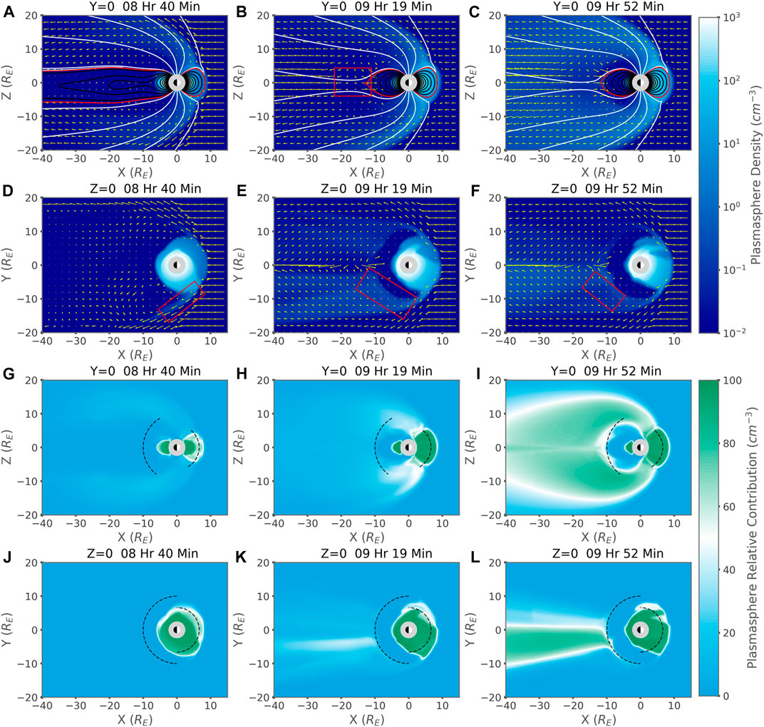
FIGURE 3. From the BATS-R-US simulation of the Ideal Square Wave Event. Column (A): 8 Hr and 40 Min into the simulation just as the plume arrives at dayside reconnection. Column (B): 9 Hr 19 Min into the simulation, when there is about equal recirculation around the flanks and over the poles. Column (C): 9 Hr 52 Min into the simulation, at the period of maximum relative contribution of the plasmasphere to total fluence across the night side measurement boundary 1. (A)–(F) State of the Plasmasphere at three key times of the Ideal Square Wave Event. The color map corresponds to the density of the plasmasphere fluid in BATS-R-US, while the yellow vector field represents the velocity of the same fluid. (A–C) Y = 0 slices additionally showing the magnetic field configuration. White curves are open magnetic field lines, red is the last closed field line, while black curves represent the closed magnetic field. (D–F) Z = 0 slices. (G–L) Relative contribution of the plasmasphere fluid to the total fluid density. A contribution of 0% means that there is no contribution to the total density from the plasmasphere fluid. A contribution of 50% means that the combined solar and polar wind fluid contributes to the total density equally with the plasmasphere fluid. A contribution of 100% means that there is no contribution to the total density from the combined solar and polar wind. The color map is scaled so that white occurs at 50%. The Black dashed circular arcs mark the where the surface of measurement crosses through the Y = 0 and Z = 0 planes 1. (G–I) Y = 0 slices, (J–L) Z = 0 slices.

Figure 3G–L shows the relative contribution of the plasmasphere fluid to the total fluid density in BATS-R-US. Figures 3G–I contains Y = 0 slices while Figure 3J–L contains Z = 0 slices. We see from the progression of Figures 3G–I that the filling of the dayside lobes with recirculating plasmasphere material takes a significant amount of time. By the time plasmasphere fluid is a significant fraction of the total population in the lobes, we see that the recirculating plasmasphere is already a significant contributor to the population of the plasma sheet (Figure 7B). In agreement with conclusions drawn from Figures 3A–F we see that the around-the-flank recirculation is must faster then over the pole recirculation. By comparing the timing of the lobes becoming dominated by the recirculated plasmasphere to Figure 7 we see that the peak of the relative contribution of the plasmasphere fluid to the total fluence from the plasma sheet into the inner magnetosphere comes during a time when through-the-lobe recirculation is dominant.

Consider the progression shown in all three time slices. We see that early in the storm, material leaks out of the plasmasphere primarily through the dawn flank, not over the lobes. While some plasmasphere material does recirculate through the dusk flank, it is a small amount compared to the recirculation through the dawn flank. This disparity is primarily due to the location of the plasmaspheric bulge being near the dawn flank when the storm began. We see that recirculation along the flanks is relatively fast compared to recirculation over the lobes as the tail begins to fill with plasmaspheric fluid from the flanks before the lobes fill with plasmaspheric material. As the storm progresses, however, we see that plasmaspheric plasma recirculating along the flanks diminishes as the dayside plume moves towards the center of the reconnection line away from the flank. At the same time, the lobes are now full and providing most of the recirculating plasma. Thus, the path that recirculating plasma takes is dependent on the location of the dayside plume and how much time has passed since the storm began. To see an animated movie of Figures 3A–F for the Ideal Square Wave simulation see the Supplementary Materials presented at the end of this paper.

The times, 08 Hr 40 Min, 09 Hr 19 Min, and 09 Hr 52 Min, are also marked on Figures 7, 8 to aid in making comparisons between plot features. These markings will be labeled ‘A.)’, ‘B.)’, and ‘C.)’, corresponding to the columns of Figure 3. In addition to these marked times, the start of the storm at 08 Hr 00 Min is also marked, though it is unlabeled.

Figure 4 shows the pressure of the fluids in BATS-R-US at the same times depicted in Figure 3. Figures 4 A–C and G–I are the pressure of the combined solar and polar wind and the plasmasphere in the Y = 0 slice, receptively. Figures 4 D–F and J–L are Z = 0 slices of the pressure of the same fluids. We see that the pressure of the combined solar wind and polar wind is much greater than that of the plasmasphere. This fact is reflected in Figure 5 where we compare the temperates. We see in Figures 4J–L that as time progresses the recirculated plasma sphere builds pressure in the tail and along the night side inner magnetosphere.

FIGURE 4

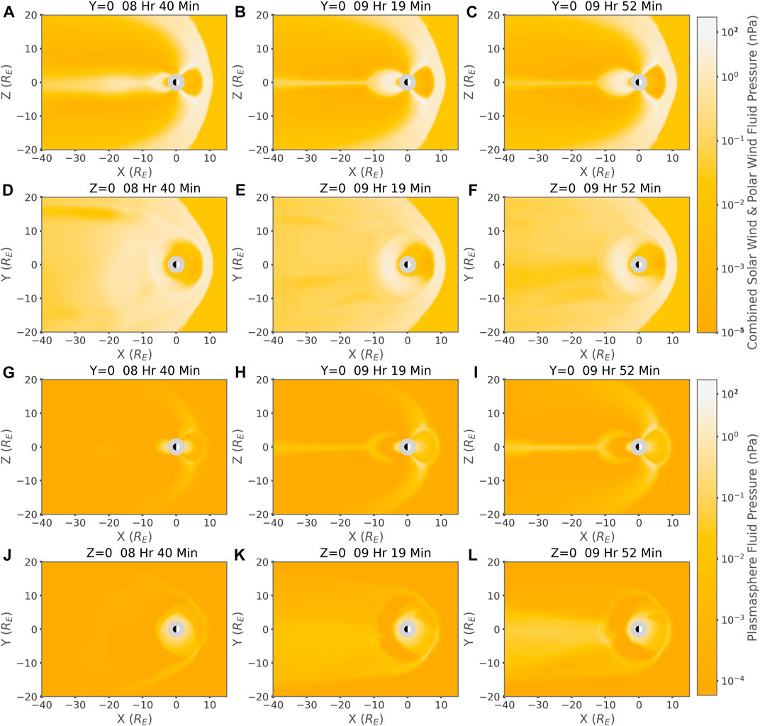
FIGURE 4. Pressure of Fluids in BATS-R-US for the Ideal Square Wave event. Column (A): 8 Hr and 40 Min into the simulation. Column (B): 9 Hr 19 Min into the simulation. Column (C): 9 Hr 52 Min into the simulation. (A–F) Pressure of the combined solar wind and ploar wind fluid. (A–C) Y = 0 slices, (D–F) Z = 0 slices. (G–L) Pressure of the plasmasphere fluid. (G–I) Y = 0 slices, (J–L) Z = 0 slices.

FIGURE 5

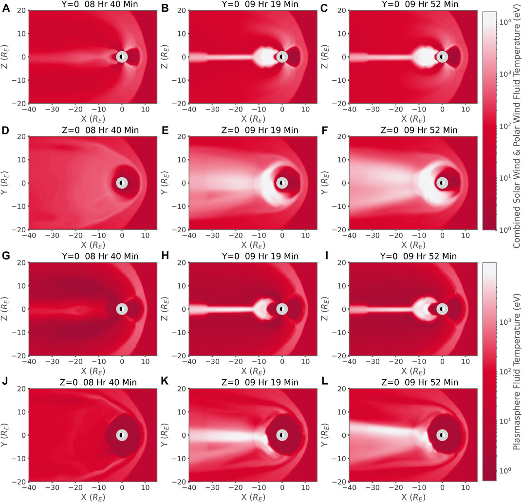
FIGURE 5. Temperature of Fluids in BATS-R-US for the Ideal Square Wave event. Column (A): 8 Hr and 40 Min into the simulation. Column (B): 9 Hr 19 Min into the simulation. Column (C): 9 Hr 52 Min into the simulation. (A–F) Temperature of the combined solar wind and ploar wind fluid. (A–C) Y = 0 slices, (D–F) Z = 0 slices. (G–L) Temperature of the plasmasphere fluid. (G–I) Y = 0 slices, (J–L) Z = 0 slices.

Figures 5A–F depicts the temperature of combined solar wind and polar wind fluid. In Figures 5G–L we see the temperature of the plasmasphere fluid. The left, center, and right columns are at the same time as those in Figure 3. The major take away from the plot is the degree to which the plasmasphere is heated during the process of recirculation. Over the entire course of leaving through the dayside plume and recirculating, plasmaspheric material is shown to heat several hundred to several thousand electron volts by the time it reenters the inner magnetosphere. This heating occurs due to several mechanisms. At the day side magnetopause pick up ion heating occurs. The plasmasphere material cools as it travels over the poles and heats again in the tail, mostly through conservation of the adiabatic invariants. Welling and Ridley 2010 discusses this process [31]. For a discussion of heating at the reconnection line Toledo-Redondo et al. 2016 and references therein discuss this [32].

Figure 6 depicts the absolute difference between the temperature of the plasmasphere fluid and the combined solar and polar wind fluid in BATS-R-US. Figures 6A–C shows Y = 0 slices while 6D-F shows Z = 0 slices. Again the left, center, and right columns correspond to 8 h 40 min, 9 h and 19 min and 9 h and 52 min after the simulation began. At all times we see a significant difference between the temperature of the plasmasphere and combined solar and polar wind. This large temperature difference occurs even in regions where the recirculating plasmaspheric plasma has been extremely heated. This difference in temperatures is crucial as it should be detectable by satellite missions such as THEMIS and CLUSTER. This feature indicates that a signature of recirculating plasma could be detected as a secondary population of plasma in the tail whose temperature is several keV below the majority of the detected plasma. The fact that this signature does not rely on tracer species, such as helium or oxygen, greatly expands the number of candidate events that can be studied in the future.

FIGURE 6

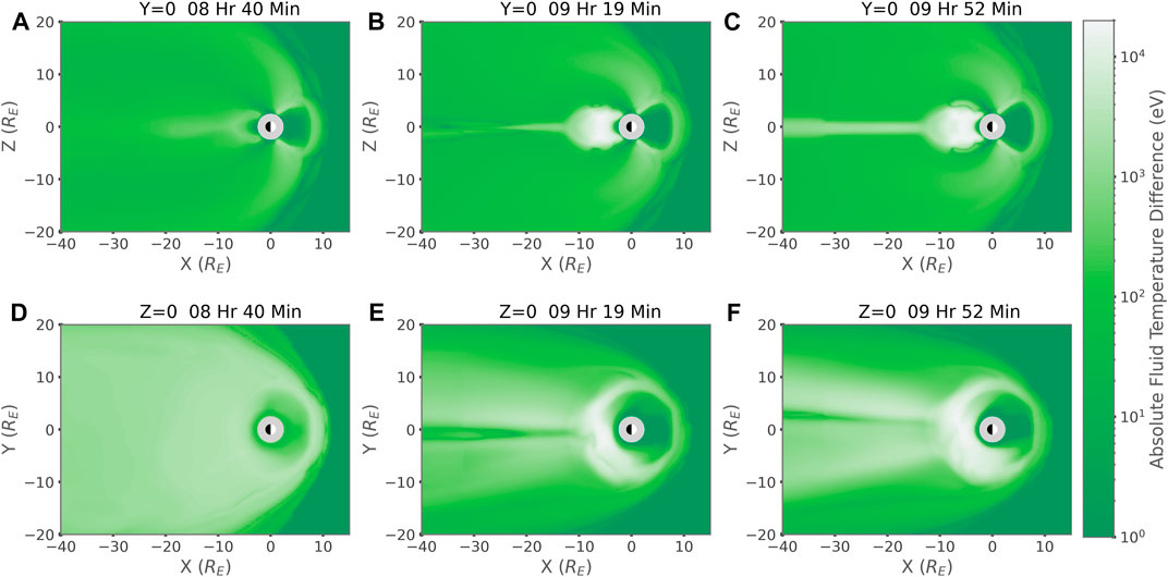
FIGURE 6. Absolute temperature difference of the plasmasphere fluid and combined solar and polar wind fluid in the BATS-R-US simulation for the Ideal Square Wave event. Column (A): 8 h and 40 min into the simulation. Column (B): 9 h 19 min into the simulation. Column (C): 9 h 52 min into the simulation. (A)–(C) Y = 0 slices, (D)–(F) Z = 0 slices.

The next value which we will look at is fluence, being the integration of flux over a surface. On the dayside of the planet, the surface of integration was a hemispherical shell going from dawn to dusk and spanning ±60° latitude at 6.6 R_E, geosynchronous orbit. The boundaries of the integration surfaces are recorded in Table 1. Fluence is calculated through the surface of the shell as a discrete sum of the flux over the area, where flux_r is the radial flux. r is the radius fixed to 6.6 R_E on the dayside. θ is the latitude and ϕ is the longitude. dθ and dϕ are the discrete step in theta and phi with values of π/90 radians due to the resolution of data points on the spherical shell. The flux is calculated from the density and bulk flow velocities of the fluids taken from BATS-R-US. On the night side, the boundary through which we measure flux and calculate fluence is a hemi spherical shell of 10 R_E going from dawn to dusk and ±30° latitude. This radial distance was chosen due to the coupling between BATS-R-US and DGCPM which occurs at and within 10 R_E. This limitation raises an issue which we will discuss later. The choice of 6.6 R_E on the dayside is somewhat arbitrary. The dayside surface was chosen to be at that distance because in both simulations the surface was never in the solar wind. Geosynchronous orbit is also were many satellites with plasma detecting instruments sit. Therefore, in the future, geosynchronous orbit is a likely place to look for signatures of plasmaspheric recirculation. Having such data now will allow us to compare directly between this current study and possible future work. On the night side, we are interested only in the fluence of the BATS-R-US fluids towards Earth. Therefore, the calculation of fluence on the night side censors flux which is pointing away from Earth. The case is reversed on the day side, where the flux pointing towards Earth is censored in the fluence calculation. The intersection of these 3D surfaces with the Y = 0 and Z = 0 planes is marked on Figures 3G–I as black dashed arc segments.

$fluence\left(\frac{\#}{s}\right)=\mathrm{\Sigma }flu{x}_r{r}^2\cos \left(\theta \right)d\theta d\varphi (4)$

TABLE 1

TABLE 1. Limits of the surface of measurement through which fluence is calculated.

Figure 7A shows the fluence of the fluids in BATS-R-US as they pass the measurement boundaries. The x-axis of Figure 7 is simulation time. We do not show the first 6 hours after the simulation began, as the early part of the simulation is simply to build a steady state in the inner magnetosphere. The y-axis of Figure 7A shows the fluence of the fluids in BATS-R-US as they pass through the measurement surfaces (Table 1). The vertical line marked ‘Ω.)’ corresponds to the start of the storm. The vertical lines marked ‘A.)’, ‘B.)’, ‘C.)’ correspond to the times: 08 h 40 min, 09 h 19 min, and 09 h 52 min. These times correspond to the left, center, and right columns of Figures 3–7 the bright green curve indicates the flow of plasmaspheric material through the dayside measurement surface, while the remaining three curves show the flow of material through the night side measurement surface. The dark green curve represents the fluence of plasmaspheric material on the night side, and thus, represents the recirculated plasmaspheric plasma. The dark blue curve shows the fluence of the combined solar and polar wind through the night side measurement surface. The dark red curve shows the total fluence of both BATS-R-US fluids through the night side measurement surface. Figure 7A shows that plasmaspheric material flows strongly out the dayside boundary, indicating a strong plume flow. This finding agrees well with observations made in the Z = 0 slices of Figure 3. The value is comparable to ionospheric outflow once the storm begins. By comparing the magnitude of the fluence of plasmaspheric material leaving the plasmasphere on the dayside to the fluence of the plasmaspheric materials crossing the night side boundary, we see that we lose an order of magnitude of material during the process of recirculation. Thus, we can state that most of the material is lost to the solar wind, which agrees well with Moore et al. (2008) [11]. Maximum fluence of the recirculated plasmaspheric material through the night side boundary occurs around 9 Hr 37 Min. Looking back to Figure 3, we see that this is in between the majority of recirculation traveling through the flanks at 09 h 19 min, or the lobes at 09 h 52 min. As might be expected, maximum recirculation occurs when the plasma has the most paths through which to travel. Note that from approximately 09 h 45 min to 10 h 30 m, the dayside plasmaspheric fluence out the plume remains fairly constant. However, at the same time, the fluence of plasmaspheric material on the night side decreases. By comparison to Figure 3, this time indicates a shift from mostly around the flank recirculation to mostly over-the-pole recirculation. Therefore, the fall off in plasmaspheric fluence on the night side indicates that recirculation through the flank is a more efficient path then over-the-pole recirculation. The spike in the solar and polar wind fluid crossing the night side boundary is explained by a build up of cold plasma on the night side due to flow patterns during quiet time. As the storm begins, the magnetosphere is disturbed injecting a large portion of this build up towards Earth as the magnetosphere collapses. After this initial spike, we see that the amount of combined solar and polar wind crossing the night side boundary is comparable to that of the plasmaspheric material which has recirculated. For a more detailed comparison of the fluid crossing the night side boundary, we look to the bottom frame of Figure 7B.

FIGURE 7

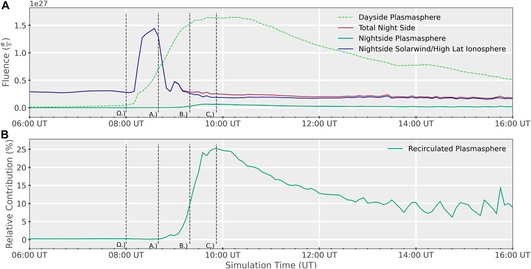
FIGURE 7. The vertical line marked ‘Ω.)’ corresponds to the beginning of the storm. The vertical lines marked ‘A.)’, ‘B.)’, ‘C.)’ correspond to the times shown in the left, center, and right columns of Figures three to six respectively. (A) Fluence of the BATS-R-US fluids as they cross the measurement boundaries on the day and night side 1. “Dayside Plasmasphere” corresponds to the fluence of the plasmasphere material through the dayside plume. “Total Night Side” refers to the total fluence of all fluids passing through the night side measurement boundary. “Nightside Solarwind/High Lat Ionosphere” refers to the fluence of the combined solar and polar wind across the night side boundary. “Nightside Plasmasphere” refers to the fluence of the recirculating plasmasphere through the night side measurement boundary. (B) Relative contribution of the recirculating plasmasphere to the total fluence crossing the night side measurement boundary in the Ideal Square Wave event 1. At 0% there is no recirculating plasmasphere, at 50% the recirculating plasmasphere is contributing equally to the combined solar and polar wind.

Figure 7B shows what percentage of the material crossing the night side boundary was provided by the recirculated plasmasphere material. The y-axis is the percentage of the total fluence which is provided by the recirculated plasmasphere. At 0% there is no plasmasphere recirculation, at 50% the recirculated plasmasphere contributes equally with the other fluid, which is the combined solar and polar winds. Once the dayside plume has vented a substantial amount of material, we see that the recaptured portion is still more then 10% of the total plasma content crossing the night side for three and a half hours. The maximum contribution of the recirculated material was 25%, with contributions over 20% lasting about an hour. Unsurprisingly, by comparison with Figure 3, we see that the maximum relative contribution occurs during the time when both flank and over-the-pole recirculated plasma was contributing to the total fluence on the night side. Refer to Figure 8 of Welling et al. (2018) [33] which shows the results of an experiment done where O⁺ was injected into the inner magnetosphere in windows centered around dawn, midnight, and dusk. As the plot there demonstrates, the more dawnward material is injected into the ring current, the more likely it is to remain on a closed drift path and contribute to the ring current. This fact raises a point which we will discuss later.

FIGURE 8

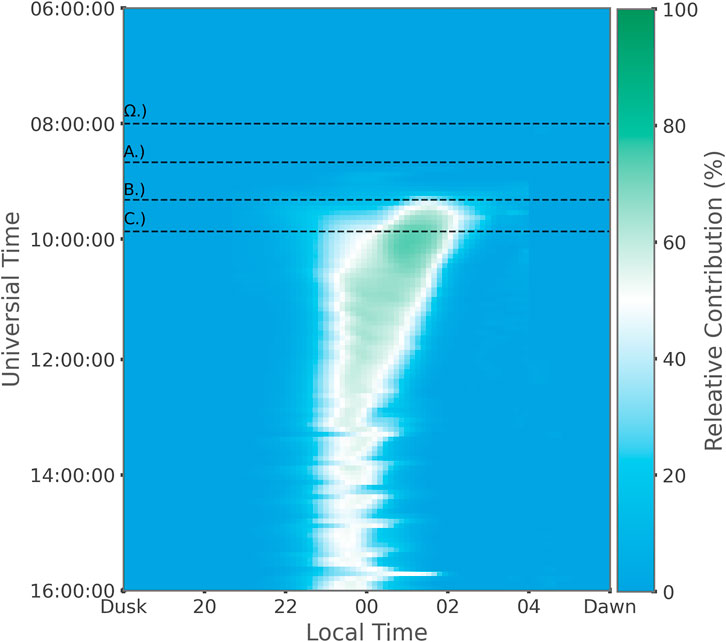
FIGURE 8. Relative contribution of the recirculating plasmasphere as a function of local time and simulation time. At 0% there is no recirculating plasmaspheric material. At 50% (white) the recirculating plasmaspheric material is contributing equally to the combined contributions of solar and polar winds. At 100% there is no contribution from the solar and polar winds. The horizontal line marked ‘Ω.)’ corresponds to the beginning of the storm. The horizontal lines marked ‘A.)’, ‘B.)’, ‘C.)’ correspond to the times shown in the left, center, and right columns of Figures three to six respectively.

A consequence of Welling et al. (2018) [33] Figure 8 is that in addition to considering the absolute contribution of the fluids in BATS-R-US to the plasma sheet, we must also consider where those contributions were made in space. Figure 8 shows what percentage of the total fluence crossing the night side measurement surface was provided by the recirculating plasmaspheric plasma, broken down by magnetic local time. The y-axis is simulation time, with the earlier parts of the simulation being at the top of the plot. The x-axis is magnetic local time going from dusk through midnight to dawn. The color map is scaled so that 0% recirculated plasmaspheric plasma corresponds to the darkest blue. At 100%, which would represent only recirculated plasmaspheric material crossing the night side boundary, the color map is the darkest green. The white color indicates 50% where recirculated plasmaspheric fluid and the combined solar and polar wind fluid are contributing equally. What we see here is that, relative to the combined solar wind and polar wind fluid, most of the contribution of the recirculated plasmaspheric material is centered in a window spanning midnight to 2 a.m. local time. The recirculated plasmaspheric plasma goes from being mostly provided by the dawn side flank, to being provided by the over-the-pole recirculation. At the same time, we see the majority contribution of the plasmaspheric plasma flow shift duskward. The duskward shift of the plasmasphere material crossing the night side boundary also corresponds with the dayside plume continuing to sweep from dawn to dusk. The recirculated plasmaspheric plasma has a local maximum contribution of 70% of the total fluence across the boundary in a window spanning midnight to 2 a.m. local time.

3.2 Idealized corotating interaction region

The second event studied for this paper is an idealized corotating interaction region (CIR). The event was constructed by taking a time averaged epoch analysis of 11 storms during solar cycle 23 [34]. For a more detailed discussion of exactly how the anaylysis was preformed see Katus et al. 2015. Figure 9 shows a detailed plot of the IMF conditions used for this simulation. All four panes of Figure 10 share an x-axis with the major ticks being periods of 24 h. Figure 9A, the top panel shows the B_y and B_z components of the IMF. The y-axis here is the displacement from quiet time averages of the IMF measured in nanotesla (nT). The storm occurs in two phases. The first phase of the storm starts after 6 h and begins as a sharp southward turning in the B_z component of the IMF of about 7.5 nT. After remaining steady for about 4 hours, there is a second southward turning in the B_z component of roughly another 7.5 nT where it remains for approximately 4 hours before beginning to recover. The idealized CIR storm has a long recovery period of 65 h [34]. As this study is only interested in the main phase of the storm, the first 30 h of the ideal CIR storm was simulated. The density of the solar wind, Figure 9B, increases from an average of 12.5/cm⁻³ up to 22.5/cm⁻³ before recovering to 12.5/cm⁻³ at the end of the storm. Figure 9C shows the velocity of the solar wind measured in km/s along the y-axis. The velocity of the solar wind began slower then that of the other simulation at 350 km/s, however, the velocity increased throughout the simulation ending at 525 km/s.

FIGURE 9

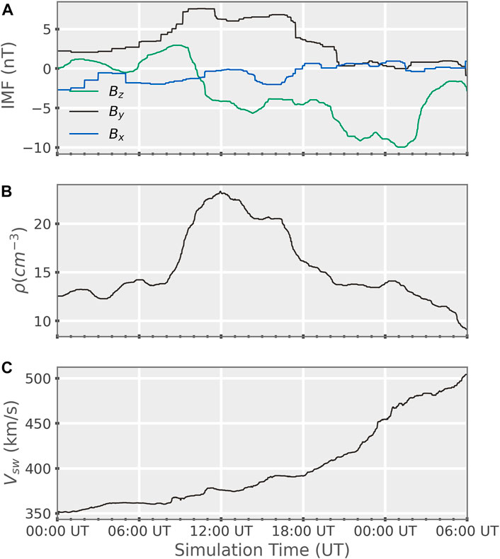
FIGURE 9. (A) Magnitude of disturbance from quiet time average of the B_z and B_y components of the IMF. (B) Density of the solar wind as a function of simulation time. (C) Velocity of solar wind as a function of simulation time.

FIGURE 10

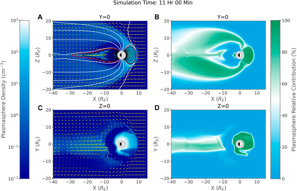
FIGURE 10. (A) Y = 0 slice showing the density of the plasmasphere fluid, plasmasphere fluid velocity vector field, and magnetic fields. White magnetic field lines are open, black are closed, and red is the last closed magnetic field line. (B) Y = 0 slice showing the relative contribution to the total density of the plasmasphere fluid. (C) Z = 0 slice showing the density of the plasmaspheric fluid, plasmaspheric fluid velocity vector field. Yellow arrows in both plots are the velocity of the plasmasphere fluid. (D) Z = 0 slice showing the relative contribution to the total density of the plasmasphere fluid. All plots are from 11 h into the Idealized CIR event simulation. This time approximately corresponds to the maximum relative contribution of the plasmasphere material to the total fluence on the night side measurement boundary.

Figure 10 reports the state of the plasmasphere in BATS-R-US for the Idealized CIR storm at 11 h. This time corresponds to the period of maximum relative contribution of the recirculated plasmasphere to the total fluence through the night side measurement boundary (Figure 11B). Figure 10A shows a 2D slice from the Y = 0 plane, while Figure 10C shows a 2D slice of the equatorial plane. The color map of Figures 10A,C is the density of the plasmaspheric fluid in BATS-R-US. The yellow arrows represent the magnitude and direction of the velocity vector field for the plasmaspheric fluid. The velocity arrows in the upstream solar wind of each plot are 450 km/s. In Figure 10A, the black contours are closed magnetic field lines (i.e. both foot points in the ionosphere), and the red contour represents the last closed magnetic field line, whereas the white contours represent open field lines. Similar to the plot shown for the Ideal Square Wave event (Figure 3), we see that the majority of the plasmaspheric material is flowing over the poles after the initial phase of the storm. There is virtually no flow of plasmaspheric plasma around the flank by this time. This lack of flow is in part due to the location of the dayside plume. Unlike in the Ideal Square Wave event, there were initially two plumes. The smaller of the plumes was present from early in the simulation venting plasmaspheric material along the dusk flank. The main plume formed as a result of the changing IMF conditions, and first impacted the dayside reconnection line around 7:00 Simulation Time. The central plume remained much broader and denser then the dusk side plume contributing the majority of the fluence on the dayside. The third dawn side plume formed as features from the night side, plasmasphere co-rotating around Earth, became stretched out on the dawn flank as a consequence of dayside reconnection. Again, we see that plasmaspheric materials flows along the flanks well before there is significant flow over the poles into the lobes. However, unlike in the Ideal Square Wave Event, we see that the peak contribution from the plasmasphere comes from a time dominated by over-the-pole flow. Interestingly, despite the dusk side plume venting material into the tail from early in the storm, there is a slight dawnward bias in the MLT where the plasmaspheric material flows down the tail towards Earth. This dawnward bias is clearly seen in Figure 10D. To see an animated movie of Figures 10A,C for the entire storm, see the Supplementary Materials. Figures 10B,D shows the relative contribution of the plasmasphere density to the total fluid density in the Y = 0 and Z = 0 planes. Similar to what we see in Figures 3G–L, by the time we reach peak relative contribution of the recirculating plasmasphere to the total density we see that the lobes are dominated by plasmasphere material. In addition, we also see that over-the-pole recirculation dominates over around-the-flank recirculation at this stage of the storm.

FIGURE 11

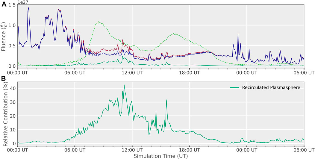
FIGURE 11. (A) Fluence of the BATS-R-US fluids as they cross the measurement boundaries on the day and night side 1. “Dayside Plasmasphere” corresponds to the fluence of the plasmasphere material through the dayside plume. “Total Night Side” refers to the total fluence of all fluids passing through the night side measurement boundary. “Nightside Solarwind/High Lat Ionosphere” refers to the fluence of the combined solar and polar wind across the night side boundary. “Nightside Plasmasphere” refers to the fluence of the recirculating plasmasphere through the night side measurement boundary. (B) Relative contribution of the recirculating plasmasphere to the total fluence crossing the night side measurement boundary in the Idealized CIR event 1. At 0% there is no recirculating plasmasphere, at 50% the recirculating plasmasphere is contributing equally to the combined solar and polar wind.

Figure 11 shows the fluence of the fluids in BATS-R-US as they pass the measurement boundaries (Table 1). The dashed bright green curve of Figure 11 is the fluence of the dayside plume, the dark red curve is the total fluence across the night side boundary, the dark green curve is the fluence of the recirculating plasmasphere on the night side, while the dark blue curve is the fluence of the combined solar and polar wind on the night side. The fluence of the dayside plume occurred in two major phases. The first phase coincided with the onset of the storm beginning around 6:00 UT. The second phase began around 14:00 UT, which coincides with the occurrence of several sub-storms in the tail. As can be seen in the animated movie included in the Supplementary Materials the relaxing of the magnetic fields after the sub-storms causes a large injection of material into the inner magnetosphere from the tail. As can also be seen by comparing Figure 11 to the animated movie of the Idealized CIR storm, as the storm progress the reconnection line on the night side moves in towards the planet. The movement of the reconnection line causes recirculating plasmasphere material to enter the tail, rather then being injected back into the inner magnetosphere. The shifting nightside reconnection line explains the lack of an increase in the recirculating plasmasphere on the night side following the period of increased fluence out the dayside seen from 14:00 UT to 20:00 UT.

Figure 11 shows the percentage of the total fluence crossing the night side boundary which is provided by the recirculating plasmaspheric plasma. The y-axis for Figure 11 is the percent relative contribution of the plasmasphere fluid. At 0% there is no recirculating plasmaspheric plasma. At 50%, the recirculating plasmaspheric plasma and combined solar and polar winds contribute equally to the fluence across the night side boundary. We note that the recirculated plasmaspheric material began to become a noticeable fraction of the whole much faster than in the Ideal Square Wave event. The relatively early increase in the importance of the recirculated plasmaspheric contribution is explained by the plasmaspheric material leaking out of the plasmasphere through the dusk side plume and into the tail through the flanks. The relative contribution is much higher than in the previous event with a maximum contribution of up to 43%. For a period of 4 hours, starting from 09:00 UT, over 20% over the total material contributing to the plasma sheet is recirculated plasmaspheric material.

Figure 12 shows what percentage of the total fluence crossing the night side measurement surface was provided by the recirculating plasmaspheric plasma, broken down by magnetic local time for the Idealized CIR event (Table 1). The y-axis is simulation time, with the earlier parts of the simulation being at the top of the plot. The x-axis is magnetic local time going from dusk through midnight to dawn. The color map is scaled so that 0% recirculated plasmaspheric plasma corresponds to the darkest blue. At 100%, which would represent only recirculated plasmaspheric material crossing the night side boundary, the color map is the darkest green. The white color indicates 50% where recirculated plasmaspheric fluid and the combined solar and polar wind fluid are contributing equally. Unlike for Figure 8 a filter is applied to the calculated relative contribution. This filter takes the form of a minimum required fluence. If the total fluence in a given cell is below 4E7 particles per second then the value is censored and set to 0% for the purposes of the color bar scale. When the total fluence is low the recirculating plasmasphere can become a significant portion of the total fluence in a cell, even dominating it. This lack of fluence causes random spikes of high contribution of the recirculating plasmasphere to appear all over the plot. Therefore, the minimum fluence requirement is imposed to not give a false sense of importance to the recirculating plasmasphere. Despite the censorship, we see several similarities to Figure 8. The most important similarity is that the majority of the plasmasphere recirculation comes in a window centered around midnight. This fact is true even in the earlier part of the storm where the recirculation was primarily happening through the dusk flank. Though unlike in Figure 8 we see a duskward, rather then dawnward bias.

FIGURE 12

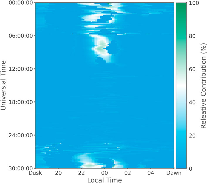
FIGURE 12. Relative contribution of the recirculating plasmasphere as a function of local time and simulation time in the Idealized CIR simulation. At 0% there is no recirculating plasmaspheric material. At 50% (white) the recirculating plasmaspheric material is contributing equally to the combined contributions of solar and polar winds. At 100% there is no contribution from the solar and polar winds.

Figure 13 shows the pressure of the fluids in BATS-R-US at the point when recirculating plasmasphere material was at it highest peak. The left column depicts the pressure of the plasmasphere fluid, while the right column depicts the combined solar and polar wind. The top row of Figure 13 contains a Y = 0 slice, while the bottom row contains a Z = 0 slice. Figure 13 shows that in the equatorial plane the combined solar and polar wind fluid has a much higher pressure then the plasmasphere fluid. The most significant source of pressure for the plasmasphere, outside the plasmasphere itself, is a beam of plasma in the night side equatorial tail centered around midnight. This region of relatively high pressure corresponds, by comparison to Figure 10, to a fast, but not dense, flow of recirculating plasma in the tail.

FIGURE 13

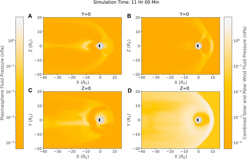
FIGURE 13. Taken from BATS-R-US at 11 h into the Idealized CIR simulation. (A, C) Y = 0 and Z = 0 slices pressure of plasmasphere fluid respectively. (B, D) Y = 0 and Z = 0 slices pressure of combined solar and polar wind fluid respectively.

Figure 14 shows how the temperature of the fluids in BATS-R-US evolve as a function of location within the environment. The image was generated from a single time corresponding to the storm maximum in the Idealized CIR event simulation. The right column shows 2D slices of the Z = 0 plane, while the left hand column shows 2D slices from the Y = 0 plane. The top row of Figure 14 shows the absolute temperature difference between the combined solar and polar wind fluid, and the plasmaspheric fluid measured in electron volts (eV). The central row depicts the temperature of the combined solar and polar wind fluid, while the bottom row depicts the temperature of the plasmaspheric fluid, both reported in electron volts (eV). In strong agreement with Figures 5, 6 we see that the plasmasphere fluid is heated to several keV in regions outside the plasmasphere. We see that the temperature difference between the combined solar and polar wind and the plasmasphere is on the scale of several keV in regions such as the tail. This finding reinforces the results of Figure 6, demonstrating that the recirculated plasmasphere could be detached independent of the solar or polar winds, with out the need of a tracer species.

FIGURE 14

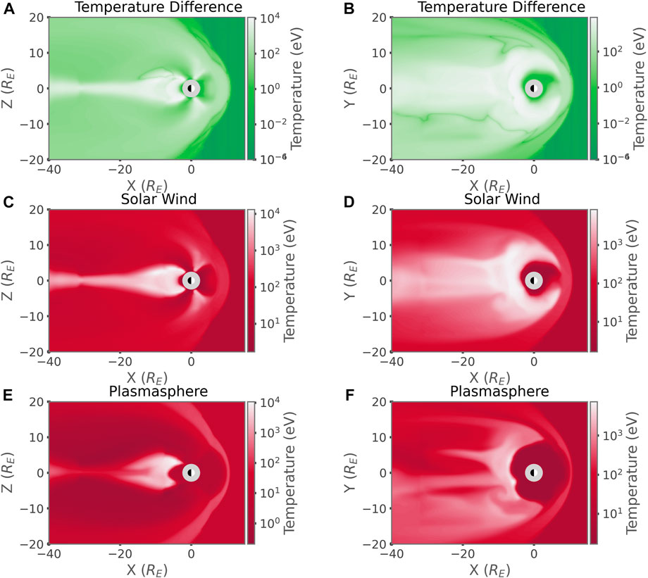
FIGURE 14. (Left Column) Y = 0 Slices, (Right Column) Z = 0 slices. (A, B) Absolute Temperature Difference between the two BATS-R-US fluids. (C, D) Temperature of the combined solar wind and polar wind fluid. (E, F) Temperature of the plasmasphere fluid.

4 Discussion

This work makes large improvements over previous studies such as the Moore et al. (2008) study. The large advancements past previous studies is the inclusion of a self-consistent plasmasphere-global MHD coupling. However, this study is limited in a key way. Due to the coupling between BATS-R-US and DGCPM, it is not possible to say how significant a contributor recirculated plasmasphere material is to the ring current. Referring back to Figure 11, note in the Z = 0 slice the region of low plasmasphere density just inside of 10 R_E on the night side. A similar phenomena is also visible in the subplots D-F in Figure 3. There is a clear and sudden fall off of plasmasphere material being injected from the tail into the night side plasmasphere and ring current. This drop of plasmasphere density is due to the nature of the coupling between BATS-R-US and DGCPM. Within 10 R_E, BATS-R-US nudges its own solution for the plasmasphere fluid density towards that calculated by DGCPM from the ion flux tube content. In BATS-R-US, once the plasmasphere fluid leaves the plasmasphere DGCPM loses track of it. At this point the dynamics of the plasmaspheric fluid are entirely determined by MHD. Thus, when plasmaspheric plasma recirculates and crosses back into the coupling region with DGCPM, BATS-R-US quickly kills the density of the plasmaspheric fluid to match DGCPM, which is unaware of material at those L-shells and local times.

Given the results of our simulations, we can state that recirculation happens within SWMF. Relative to the solar wind and high latitude ionosphere outflow, the recirculating plasmaspheric plasma is non-negligible. Due to the coupling of BATS-R-US and DGCPM, we cannot state the exact affect the recirculating plasmaspheric plasma has on the ring current. It should be possible to use the results of these two simulations to drive a ring current model. This simulation would allow us to test the magnitude of the contribution provided by recirculating plasmaspheric plasma to the ring current. To serve as a control case, storms both with and without dayside plumes would be required. In keeping with the idea of self-consistency, however, it would be preferable to add a ring current into the SWMF configuration laid out in Figure 1 and have it couple both to the plasmasphere and MHD codes.

5 Conclusion

We performed two simulations using the SWMF configured with a global MHD, plasmasphere, and ionosphere models. In each simulation, we saw that material from the plasmasphere does recirculate into the inner magnetosphere and provides anywhere from ten to forty percent of the total material entering the inner magnetosphere from the tail. Therefore, we can state that recirculating plasmaspheric plasma is a non-negligible, possibly significant, contributor to the ring current. Other findings include that most of the plasmaspheric material was lost to the solar wind in both simulations, which is in agreement with the Moore et al. (2008) study. We found that the path of recirculation was dependent on the location of the dayside plume. Additionally, we found that the path of recirculation would evolve as the storm progressed. Early in the storm recirculation around the flanks was favored, while latter in the storm over-the-pole recirculation was dominant. The pre-storm and storm conditions can have a significant impact on the relative contribution of the plasmasphere. We also found that during the process of recirculation the plasmasphere material can be heated anywhere from several hundred eV to several keV, which is a greater heating effect then seen in earlier studies.

Data availability statement

The original contributions presented in the study are included in the article/Supplementary Materials, further inquiries can be directed to the corresponding author.

Author contributions

C-AB-W: Primary Author, graduate student. Paper covers first 3 years of graduate work DW: Graduate Advisor. Helped with interpretation of data, editing, and writing portions of the paper. RL: Graduate Advisor. Helped with interpretation of data, editing, and writing portions of the paper. RK: Provided IMF storm conditions for use in a simulation presented in this work BW: advised group on plasmasphere dynamics.

Funding

This work was supported by grants from the NSF (award AGS 1502436) and NASA (award 80NSSC21K2057).

Conflict of interest

The authors declare that the research was conducted in the absence of any commercial or financial relationships that could be construed as a potential conflict of interest.

Publisher’s note

All claims expressed in this article are solely those of the authors and do not necessarily represent those of their affiliated organizations, or those of the publisher, the editors and the reviewers. Any product that may be evaluated in this article, or claim that may be made by its manufacturer, is not guaranteed or endorsed by the publisher.

Supplementary material

The Supplementary Material for this article can be found online at: https://www.frontiersin.org/articles/10.3389/fphy.2023.1146035/full#supplementary-material

Abbreviations

BATS-R-US, Block-Adaptive-Tree-Solarwind-Roe-Upwind-Scheme; CRCM, Comprehensive Ring Current Model; CIR, Corotating Interaction Region; DGCPM, Dynamic Global Core Plasma Model; R_E, Earth Radii; IMF, Interplanetary Magnetic Field; LFM, Lyon-Fedder-Mobarry; MHD, magnetohydrodynamic; RIM, Ridely Ionosphere Model; SWMF, Space Weather Modeling Framework.

References

1. Singh AK, Singh RP, Siingh D. State studies of earths plasmasphere: A review. Planet Space Sci (2011) 59:810–34. doi:10.1016/j.pss.2011.03.013

CrossRef Full Text | Google Scholar

2. Dungey JW. Interplanetary magnetic field and the auroral zones. Phys Rev Lett (1961) 6:47–8. doi:10.1103/PhysRevLett.6.47

CrossRef Full Text | Google Scholar

3. Su YJ, Borovsky JE, Thomsen MF, Dubouloz N, Chandler MO, Moore TE, et al. Plasmaspheric material on high-latitude open field lines. J Geophys Res Space Phys (2001) 106:6085–95. doi:10.1029/2000JA003008

CrossRef Full Text | Google Scholar

4. Walsh BM, Phan TD, Sibeck DG, Souza VM. The plasmaspheric plume and magnetopause reconnection. Geophys Res Lett (2014) 41:223–8. doi:10.1002/2013GL058802

CrossRef Full Text | Google Scholar

5. Freeman JW, Hills HK, Hill TW, Reiff PH, Hardy DA. Heavy ion circulation in the earth’s magnetosphere. Geophys Res Lett (1977) 4:195–7. doi:10.1029/GL004i005p00195

CrossRef Full Text | Google Scholar

6. Borovsky JE, Thomsen MF, McComas DJ. The superdense plasma sheet: Plasmaspheric origin, solar wind origin, or ionospheric origin? J Geophys Res Space Phys (1997) 102:22089–97. doi:10.1029/96JA02469

CrossRef Full Text | Google Scholar

7. Daglis LA, Thorne RM, Baumjohann W, Orsini S, Daglis IA, Thorne RM, et al. The terrestrial ring current: Origin, formation, and decay. Rev Geophys (1999) 37:407–38. doi:10.1029/1999RG900009

CrossRef Full Text | Google Scholar

8. Elphic RC, Thomsen MF, Borovsky JE. The fate of the outer plasmasphere. Geophys Res Lett (1997) 24:365–8. doi:10.1029/97GL00141

CrossRef Full Text | Google Scholar

9. Weimer DR. A flexible, imf dependent model of high-latitude electric potentials having “space weather” applications. Geophys Res Lett (1996) 23:2549–52. doi:10.1029/96GL02255

CrossRef Full Text | Google Scholar

10. Tsyganenko N. A magnetospheric magnetic field model with a warped tail current sheet. Planet Space Sci (1989) 37:5–20. doi:10.1016/0032-0633(89)90066-4

CrossRef Full Text | Google Scholar

11. Moore TE, Fok MC, Delcourt DC, Slinker SP, Fedder JA. Plasma plume circulation and impact in an mhd substorm. J Geophys Res Space Phys (2008) 113. doi:10.1029/2008JA013050

CrossRef Full Text | Google Scholar

12. Ober DM, Daniel M, Ober JL, Horwitz DG. Formation of density troughs embedded in the outer plasmasphere by subaruroral ion drift events. J Gphysical Res (1997) 102:14595–602. doi:10.1029/97JA01046

CrossRef Full Text | Google Scholar

13. Huba J, Krall J. Modeling the plasmasphere with Sami3. Geophys Res Lett (2013) 40:6–10. doi:10.1029/2012GL054300

CrossRef Full Text | Google Scholar

14. Tóth G, Sokolov IV, Gombosi TI, Chesney DR, Clauer CR, De Zeeuw DL, et al. Space weather modeling framework: A new tool for the space science community. J Geophys Res Space Phys (2005) 110:A12226. doi:10.1029/2005JA011126

CrossRef Full Text | Google Scholar

15. Glocer A, Welling D, Chappell CR, Toth G, Fok MC, Komar C, et al. A case study on the origin of near-earth plasma. J Geophys Res Space Phys (2020) 125. doi:10.1029/2020JA028205

CrossRef Full Text | Google Scholar

16. Welling DT, Ridley AJ. Validation of swmf magnetic field and plasma. Space Weather (2010) 8. doi:10.1029/2009SW000494

CrossRef Full Text | Google Scholar

17. Welling DT, Liemohn MW. The ionospheric source of magnetospheric plasma is not a black box input for global models. J Geophys Res Space Phys (2016) 121:5559–65. doi:10.1002/2016JA022646

CrossRef Full Text | Google Scholar

18. Ridley A, Dodger AM, Liemohn MW. Exploring the efficacy of different electric field models in driving a model of the plasmasphere. J Geophys Res Space Phys (2014) 119:4621–38. doi:10.1002/2014JA019836

CrossRef Full Text | Google Scholar

19. Ridley AJ, Gombosi TI, DeZeeuw DL. Ionospheric control of the magnetosphere: Conductance. Ann Geophysicae (2004) 22:567–84. doi:10.5194/angeo-22-567-2004

CrossRef Full Text | Google Scholar

20. Welling D. Magnetohydrodynamic models of B and their use in GIC estimates. American Geophysical Union (2019). p. 43–65. chap. 3. doi:10.1002/9781119434412.ch3

CrossRef Full Text | Google Scholar

21. Welling DT, Liemohn MW. Outflow in global magnetohydrodynamics as a function of a passive inner boundary source. J Geophys Res Space Phys (2014) 119:2691–705. doi:10.1002/2013JA019374

CrossRef Full Text | Google Scholar

22. Jorgensen AM, Heilig B, Vellante M, Lichtenberger J, Reda J, Valach F, et al. Comparing the dynamic global core plasma model with ground-based plasma mass density observations. J Geophys Res Space Phys (2017) 122:7997–8013. doi:10.1002/2016JA023229

CrossRef Full Text | Google Scholar

23. Carpenter DL, Anderson RR. An isee/whistler model of equatorial electron density in the magnetosphere. J Geophys Res Space Phys (1992) 97:1097–108. doi:10.1029/91JA01548

CrossRef Full Text | Google Scholar

24. Tóth G, van der Holst B, Sokolov IV, De Zeeuw DL, Gombosi TI, Fang F, et al. Issue: Computational Plasma Physics, 231 (2012). p. 870–903. doi:10.1016/j.jcp.2011.02.006.SpecialAdaptive numerical algorithms in space weather modelingJ Comput Phys

CrossRef Full Text | Google Scholar

25. Darrouzet F, De Keyser J. The dynamics of the plasmasphere: Recent results. J Atmos Solar-Terrestrial Phys (2012) 99:53–60. doi:10.1016/j.jastp.2012.07.004

CrossRef Full Text | Google Scholar

26. Moen J, Brekke A. The solar flux influence on quiet time conductances in the auroral ionosphere. Geophys Res Lett (1993) 20:971–4. doi:10.1029/92GL02109

CrossRef Full Text | Google Scholar

27. Frahm RA, Winningham JD, Sharber JR, Link R, Crowley G, Gaines EE, et al. The diffuse aurora: A significant source of ionization in the middle atmosphere. J Geophys Res Atmospheres (1997) 102:28203–14. doi:10.1029/97JD02430

CrossRef Full Text | Google Scholar

28. Newell PT, Sotirelis T, Liou K, Meng CI, Rich FJ. A nearly universal solar wind-magnetosphere coupling function inferred from 10 magnetospheric state variables. J Geophys Res Space Phys (2007) 112. doi:10.1029/2006JA012015

CrossRef Full Text | Google Scholar

29. Newell PT, Sotirelis T, Wing S. Diffuse, monoenergetic, and broadband aurora: The global precipitation budget. J Geophys Res Space Phys (2009) 114. doi:10.1029/2009JA014326

CrossRef Full Text | Google Scholar

30. Richmond AD, Kamide Y. Mapping electrodynamic features of the high-latitude ionosphere from localized observations: Technique. J Geophys Res Space Phys (1988) 93:5741–59. doi:10.1029/JA093iA06p05741

CrossRef Full Text | Google Scholar

31. Welling DT, Ridley AJ. Exploring sources of magnetospheric plasma using multispecies mhd. J Geophys Res Space Phys (2010) 115. doi:10.1029/2009JA014596

CrossRef Full Text | Google Scholar

32. Toledo-Redondo S, André M, Vaivads A, Khotyaintsev YV, Lavraud B, Graham DB, et al. Cold ion heating at the dayside magnetopause during magnetic reconnection. Geophys Res Lett (2016) 43:58–66. doi:10.1002/2015GL067187

CrossRef Full Text | Google Scholar

33. Welling DT, Jordanova VK, Zaharia SG, Glocer A, Toth G. The effects of dynamic ionospheric outflow on the ring current. J Geophys Res Space Phys (2011) 116:1–15. doi:10.1029/2010JA015642

CrossRef Full Text | Google Scholar

34. Katus RM, Liemohn MW, Ionides EL, Ilie R, Welling D, Sarno-Smith LK. Statistical analysis of the geomagnetic response to different solar wind drivers and the dependence on storm intensity. J Geophys Res Space Phys (2015) 120:310–27. doi:10.1002/2014JA020712

CrossRef Full Text | Google Scholar