An improved approach for rapid filter convergence of GNSS satellite real-time orbit determination

1 Introduction

Since the announcement of global BeiDou navigation system (BDS-3) operation by the Chinese government in July 2020, there have been 137 global navigation satellite system (GNSS) satellites in operation, including GPS, Galileo, GLONASS, and BDS, until December 2022 (https://igs.org/mgex/constellations/). Numerous GNSS satellites provide plenty of observations for a better performance of positioning, navigation, and timing service. The GNSS satellite precise orbit is the basic requirement for high-accuracy applications such as precise point positioning (PPP) and precise time transfer [20, 28].

The batch processing method is generally used to calculate precise orbit products. It uses observations from globally distributed stations and calculates the state parameters together with the dynamic parameters through least square estimation. Using the batch processing method, the one-dimensional (1D) orbit accuracy of GPS satellites from the International GNSS Service (IGS) final product is better than 2.5 cm [27]. For multi-GNSS satellites, a consistency between different IGS Multi-GNSS Experiment (MGEX) analysis centers in three-dimensional (3D) is 6–17 cm for GLONASS, 14–29 cm for Galileo, and 12–26 cm, 32–51 cm, and 5 m for BDS medium Earth orbit (MEO), inclined geosynchronous orbit (IGSO), and geostationary orbit (GEO) satellite, respectively [16]. The predicted orbit is usually broadcast to users as the real-time orbit. At present, the ultra-rapid orbit product provided by IGS is broadcast via Internet every 6 h, including 24-h measured orbit and 24-h predicted orbit. The 3D root mean square (RMS) of the predicted GPS orbit is less than 5 cm [24]. For multi-GNSS satellites, a previous study showed that the accuracy of GPS, Galileo, and BDS-2 satellites of ultra-rapid products from the International GNSS Monitoring and Assessment System (iGMAS) is 5.7 cm, 14.2 cm, and 18.0 cm with respect to the IGS final product (Xu et al. 2020), respectively. Although the batch processing method can provide the real-time orbit at the centimeter level, this approach is not the most suitable for real-time applications. On one hand, the orbit accuracy will be greatly decreased after a long time of integration if the initial state of satellites or the force model is not accurate enough. This is especially noticeable for BDS-2 satellites in the orbit-normal mode [4]. On the other hand, the batch processing method cannot handle the satellite in maneuver in real time [3]. In addition, batch processing algorithm needs to store a huge amount of observation data for calculation, resulting in a low computational efficiency [25].

In order to overcome the problems mentioned previously, an alternative method is to use the filter method to provide stable and precise real-time orbit to users. It updates the orbit state in real time, and parameters of the solar radiation pressure (SRP) model can be processed more flexibly and better adjusted to the influence on orbit brought by the change in SRP. Using the filter method, the Jet Propulsion Laboratory (JPL) has developed the Global Differential GPS to provide real-time products of GPS and GLONASS since 2000 [18]. RTG/RTGX software from JPL uses square root information filter (SRIF) to determine the real-time orbit and achieves a 3D accuracy of 6.4 cm for GPS. The Trimble Company developed a CenterPoint RTX Service System with centimeter-level accuracy using the Kalman filter [9]. Comparing with the IGS final product, the 3D accuracy for GPS and GLONASS satellites is 2.7 cm and 5.3 cm [9], respectively. In addition, Auto-BAHN software developed by the European Space Agency (ESA) uses the extended-Kalman filter to determine the real-time orbit of GPS, and the mean 3D-RMS is approximately 13.6 cm [26]. However, the defect of the filter method is that the orbit will undergo a convergence process costing more than 10 h in the initial stage, which brings a bad experience to real-time users.

Some studies have made contributions to reduce the convergence time of the filter method. By estimating the orbit with ambiguity resolution, the convergence time for GPS satellites can be reduced to 2.75 h, 3.25 h, and 4.5 h in the along-track, cross-track, and radial directions [13], respectively. However, the convergence time is still relatively long. By using the ultra-rapid product as the initial orbit and setting a proper a priori standard deviation (STD) of the initial states, the convergence time for BDS satellites can reach the accuracy of decimeter-level in a few minutes [19]. In general, the a priori STD is determined empirically, which lacks universality for different situations. In addition, only the a priori STD of BDS satellites is discussed while GPS and Galileo satellites are not included. [5] proposed a method of using the ultra-rapid product as the external constraint to improve the orbit convergence performance of BDS-2 satellites. By setting the constraint variation of position parameters and velocity parameters at 0.5 m and 0.5 mm/s, there is no convergence phenomenon for BDS-2 IGSO and MEO satellites. However, the stochastic model of the constraint equation is still determined empirically, which lacks theoretical foundation.

In this study, we propose an improved approach for rapid filter convergence of GNSS satellite real-time orbit determination to solve the aforementioned problems. In this approach, the ultra-rapid orbit products are introduced as external constraints where the stochastic model of the constraint equation is established by analyzing differences between the predicted part of the ultra-rapid orbit and the SRIF orbit after convergence. The constraint equation is then added to the observation equation at every epoch during the constraint period to strengthen the structure of the information matrix. This paper is organized as follows: in Section 2, the details of the proposed method are first described. Then, the experiment of real-time orbit determination without external constraints is carried out for GPS, Galileo, and BDS-3 satellites. Afterward, the differences between the ultra-rapid product and the SRIF orbit after convergence are analyzed to establish the stochastic model of the constraint equation. The constant stochastic and time-dependent stochastic models of the constraint equation are proposed and determined. Finally, the experiments of real-time orbit determination with external constraints from different schemes of constraint models are implemented to analyze the convergence performance. In Section 3, we analyze the results of our proposed method. Lastly, we discuss the results in Section 4 and show that our proposed method can effectively reduce the convergence time without damaging the orbit accuracy after convergence.

2 Materials and methods

In this section, we first introduce the function model of real-time orbit determination with external constraints. Then, a time-dependent stochastic model of the constraint equation is derived. Afterward, the implementation of the proposed method is described in a flowchart. Finally, the data collection and processing strategy are introduced.

2.1 Real-time precise orbit determination without external constraints

After solving the motion equation, the state equation for orbit determination can be expressed as follows:

$x_{t_i}^s={\Phi }^s\left(t_i,t_{i-1}\right)*x_{t_{i-1}}^s,(1)$

$x_{t_i}^s=X_{t_i}^s-{\stackrel{\sim }{X}}_{t_i}^s,(2)$

where $s$ is the satellite pseudo-random noise (PRN) code; $t_{i-1}$ and $t_i$ are the previous epoch time and the current epoch time, respectively; $X_{t_i}^s$ represents the orbit state which is a vector that includes satellite position, satellite velocity, and SRP model parameters; ${\stackrel{\sim }{X}}_{t_i}^s$ denotes the reference orbit state derived from numerical orbital integration; $x_{t_i}^s$ is the correction relative to the reference orbit parameters at the epoch time $t_i$; and ${\mathrm{\Phi }}^s\left(t_i,t_{i-1}\right)$ represents the orbit state transition matrix from the previous epoch time $t_{i-1}$ to current epoch time $t_i$.

Using the observation from continuous arcs of BDS/GNSS satellites, the real-time orbit state parameters of satellites can be determined. Through combining the original phase observation and the pseudo-range observation to eliminate the first order of ionosphere delay, the observation equations at the current epoch time $t_i$ are obtained after linearization at the reference orbit ${\stackrel{\sim }{X}}_{t_i}^s$ as follows:

$V_{P_{t_i,r,if}^s}=-l_{t_i,r}^s{x}_{t_i,r}+l_{t_i,r}^s{x}_{t_i}^s+c\left(t_{t_i,r}-t_{t_i}^s\right)+M_{t_i,r}^s{T}_{t_i,r},(3)$

$V_{L_{t_i,r,if}^s}=-l_{t_i,r}^s{x}_{t_i,r}+l_{t_i,r}^s{x}_{t_i}^s+c\left(t_{t_i,r}-t_{t_i}^s\right)+N_{t_i,r}^s+M_{t_i,r}^s{T}_{t_i,r},(4)$

where $r$ is the station ID; $V_{P_{t_i,r,if}^s}$ is the observation minus calculation (OMC) of the pseudo-range using the ionosphere-free (IF) combination; $V_{L_{t_i,r,if}^s}$ is the phase OMC using the IF combination; $l_{t_i,r}^s$ is the unit direction vector from the receiver to satellite; $x_{t_i,r}$ is the correction of the station coordinate relative to its initial value; and $t_{t_i,r}$ and $t_{t_i}^s$ denote the receiver clock bias and satellite clock bias, respectively. Note that the hardware delays in pseudo-range observation are included in receiver and satellite clock biases. Thus, they are not shown in the equation. $c$ denotes the speed of light; $M_{t_i,r}^s$ is the tropospheric projection function; $T_{t_i,r}$ is the zenith tropospheric delay (ZTD); and $N_{t_i,r,if}^s$ is the phase ambiguity that includes phase hardware delays.

All parameters in Eqs 3, 4 can be estimated at every processing epoch through filter techniques. For real-time orbit determination, there are several filter models which are usually adopted, such as the extended-Kalman filter and adaptive robust filter. We use SRIF to estimate the orbit state parameters at every processing epoch. This is because the SRIF adopts the square root matrix, and the element length is only half of the element length of the Kalman filter. Thus, the SRIF is more stable than the Kalman filter in numerical value [25].

Due to the restriction of factors such as a priori accuracy and geometry structure, the SRIF orbit parameter usually needs a long convergence time to reach high accuracy. Considering that the orbit parameter is constrained by the dynamic model with a strong regularity, the orbit parameter from the ultra-rapid orbit products can be introduced as the external constraint [5]. In this way, the solution to the equation is enhanced. The constraint equation can be expressed as

$V_{x,t_i}^s=x_{t_i}^s-{\overline{x}}_{t_i}^s,(5)$

${\overline{x}}_{t_i}^s={\overline{X}}_{t_i}^s-{\stackrel{\sim }{X}}_{t_i}^s,(6)$

where ${\overline{X}}_{t_i}^s$ represent the orbit state parameter of the ultra-rapid orbit at the current epoch time $t_i$; ${\overline{x}}_{t_i}^s$ is the difference between the ultra-rapid orbit and the reference orbit; and $V_{x,t_i}^s$ is the OMC of the constraint equation where the corresponding STD is ${\sigma }_{Vx}$.

The radial, transverse, and normal (RTN) coordinate system is usually used to measure the difference between the ultra-rapid orbit and the filter orbit. The proposed constraint equation is hence implemented in the radial, transverse, and normal (RTN) coordinate system. However, the Earth-centered inertial (ECI) coordinate system is generally adopted in precise orbit determination (POD) for a better realization of orbit integration. Therefore, we need to transform the constraint equation from the RTN coordinate system to the ECI coordinate system. Assume that the parameter vector is expressed as $V_{x,RTN}$ in the RTN coordinate system, while the corresponding vector in the ECI coordinate system is expressed as $V_{x,ECI}$. The current position and velocity vectors in the ECI coordinate system are expressed as $r$ and $\dot{r}$, respectively. Thus, the rotation matrix from the RTN coordinate system to the ECI coordinate system is

$\left\{\begin{array}{l}{g}_1=\frac{r}{\left|r\right|},\\ g_3=-r\times \dot{r}/\left|r\times \dot{r}\right|,\\ g_2=g_1\times g_3,\\ G={\left(g_1,g_2,g_3\right)}^T.\end{array}\right.(7)$

Consequently, the constraint equation in the ECI coordinate system is shown in Eq. 8. For brevity, the epoch time $t_i$ is omitted in the equation.

$V_{x,ECI}^s=G\bullet V_{x,RTN}^s.(8)$

2.2 The stochastic model of the constraint equation

From Eq. 5, we can see that the SRIF orbit parameter can be estimated closely to the parameter of the a priori orbit by constructing the constraint equation. The proximity depends on the STD ${\sigma }_{Vx}$, and the convergence performance is expected to be improved after the SRIF starts. There is no doubt that the precise determination of ${\sigma }_{Vx}$ is key to improving the convergence performance. Substituting Eqs 2, 6 into Eq. 5, the constraint equation can be rewritten as follows:

$V_{x,t_i}^s=X_{t_i}^s-{\overline{X}}_{t_i}^s.(9)$

Eq. 9 indicates that the OMC of the virtual equation is actually the difference between the orbit state and the ultra-rapid orbit products. By averaging the root mean square (RMS) of the differences for all satellites, the STD ${\sigma }_{Vx}$ can be approximately determined and is equal to a constant value for all satellites. Therefore, the constant stochastic model of the constraint equation can be established as follows:

$V_{x,RMS}^s=\sqrt{\frac{{\sum }_{i=1}^{n_t}{\left(V_{x,t_i}^s\right)}^2}{n_t},}(10)$

${\sigma }_{Vx}=\frac{{\sum }_{s=1}^{n_s}\left(V_{x,RMS}^s\right)}{n_s},(11)$

where n_t is the number of epochs to be averaged and n_s is the number of satellites for each system.

Note that the accuracy of the ultra-rapid orbit products would be decreased over time, while it is not rigorous to take ${\sigma }_{Vx}$ as a constant value during the convergence period. Therefore, a time-dependent stochastic model related to time $t$ is further proposed to simulate the time-varying value of ${\sigma }_{Vx}$, as shown in Eqs 12, 13. The function expression of Eq. 13 should be determined after analysis of the differences between the SRIF orbit state and the ultra-rapid orbit products for all satellites.

$V_{x,t_i}=\frac{{\sum }_{s=1}^{n_s}\left(V_{x,t_i}^s\right)}{n_s},(12)$

${\sigma }_{Vx}=f\left(t,V_{x,t_i}\right).(13)$

Same as the OMC value of the constraint equation, the model of Eqs 11, 13 is usually determined in the RTN coordinate system. It should be transformed to the ECI coordinate system. According to the variance–covariance propagation law, the STD of the OMC of the constraint equation in the ECI coordinate system is expressed as follows:

${\sigma }_{Vx,ECI}=\sqrt{G\bullet {\sigma }_{Vx,RTN}^2\bullet G^T.}(14)$

2.3 Implementation of the proposed method

The proposed method is implemented in five steps. First, the ultra-rapid orbit product is used to obtain the initial orbit state of BDS/GNSS satellites, and the time length of constraint period is chosen. Second, the orbit state parameters are integrated to the current time according to Eq. 1. Meanwhile, all the observation data from globally distributed ground stations are collected to form the observation equations based on Eqs 3, 4. Then, the constraint equation is constructed and introduced to the POD process using Eq. 5. Afterward, the SRIF is used to estimate orbit state parameter correction and update orbit parameter at every processing epoch. Finally, the orbit parameters are estimated without constraints after the constraint period. The flowchart of the aforementioned steps is shown in Figure 1.

FIGURE 1

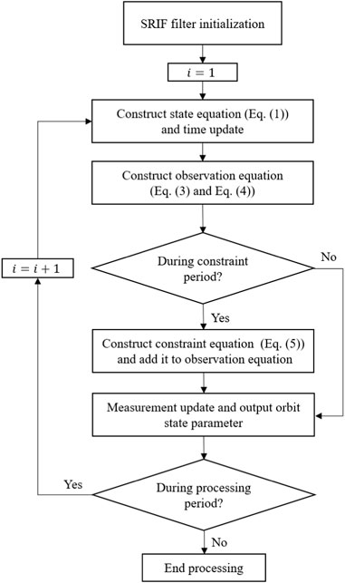
FIGURE 1. Flowchart of the proposed method for rapid filter convergence of GNSS satellite real-time POD.

In addition, if the predicted part of the ultra-rapid orbit is not of good quality (e.g., satellite maneuver), we have proposed a quality control strategy based on the statistics of the post-fit residual. The variance of unit weight of post-fit residual is first calculated in every epoch. If the result is larger than a threshold (e.g., 5.0), we calculate the residuals of ground stations toward every satellite. Then, if the percentage of ground stations with a large residual is more than a threshold (e.g., 70%), the weight of this satellite should be lowered to avoid bad values.

2.4 Data collection and processing strategies

A total number of 80 globally distributed Multi-GNSS Experiment (MGEX) stations are selected in our experiment. All these stations are able to track GPS, Galileo, and BDS-3 satellites from DOY (day of the year) 275 to DOY 302 in 2020. The global distribution of these stations is shown in Figure 2. Data processing strategies for real-time POD used in the experiments are shown in Table 1. Note that all available GPS and Galileo satellites are used for POD, while only MEO satellites of BDS-3 are included.

FIGURE 2

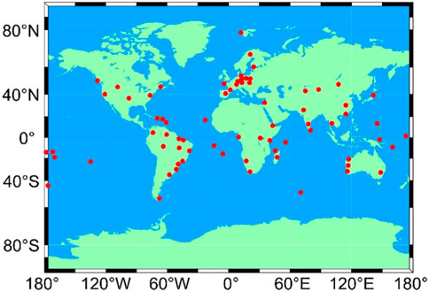
FIGURE 2. Global distribution of 80 selected IGS MGEX stations.

TABLE 1

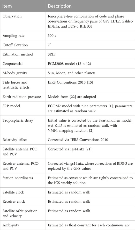
TABLE 1. Data processing strategies for real-time POD.

In order to make a comparison, we design three schemes to evaluate the convergence performance of each system, i.e., GPS, Galileo, and BDS-3. The first scheme is to estimate the orbit without external constraints. We consider the convergence performance as the reference to evaluate the enhancement of the proposed method. The second scheme is to estimate the orbit by introducing constraints to the constant stochastic model. In this scheme, we conduct the experiment with external constraints from the ultra-rapid orbit products, where the STD of the OMC of the constraint equation is chosen as a constant value by averaging the RMS of the differences between the predicted part of the ultra-rapid orbit and the SRIF orbit in different time ranges (see Eq. 11). The third scheme is to estimate the orbit by introducing constraints to a time-dependent stochastic model. In contrast to the second scheme, we use Eq. 13 to determine the time-dependent values of the STD of the OMC of the constraint equation. For each scheme, the convergence time and the orbit accuracy during and after the convergence would be evaluated and compared.

3 Results

In this section, we first implement real-time POD without external constraints to analyze the convergence time and orbit accuracy after convergence. Then, we determine the expression of both the constant stochastic model and the time-dependent stochastic model of the constraint equation by analyzing the differences between the SRIF orbit after convergence and the predicted part of the ultra-rapid orbit. Finally, we conduct the real-time POD with external constraint equations from the constant stochastic model and the time-dependent stochastic model to evaluate the convergence time and orbit accuracy.

3.1 Real-time POD without external constraints

The convergence time and the corresponding accuracy after convergence are evaluated for the real-time POD without external constraints. Precise orbit products released by Wuhan University (WUM) are taken as the reference for this evaluation. The time series of the RMS in the along-track, cross-track, and radial directions for all satellites of each GPS, Galileo, and BDS-3 constellation are shown in Figure 3. The convergence criteria for each system is that the RMSs of the along-track, cross-track, and radial directions are below 0.25 m, 0.15 m, and 0.15 m, respectively, which is shown by the dotted curve in the figure .

FIGURE 3

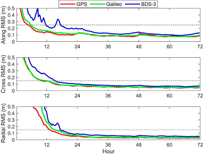
FIGURE 3. RMS time series of orbit differences for all satellites of each GNSS constellation with respect to the WUM products.

Figure 3 shows that all GPS, Galileo, and BDS-3 satellites take a long time to converge to a stable state. By comparing between different systems, GPS satellite has the shortest convergence time, while BDS-3 satellite has the longest convergence time. The reason may be that there are more ground observation stations that can track GPS and Galileo satellites, leading to a better geometric configuration. On the contrary, the distribution of ground observation stations for different BDS satellites is less uniformly distributed than that of GPS and Galileo satellites. In addition, the SRP model is more precise for GPS and Galileo satellites. This has been proved by the fact that the orbit accuracy of GPS and Galileo satellites is better than that of BDS satellites using the batch processing method [11]. Therefore, the SRIF orbit accuracy of BDS satellites is relatively poorer, and it needs longer convergence time. In addition, it can be found that the time series of the RMS will confront a discontinuity at 24 h and 48 h. Among three satellite systems, the discontinuity of Galileo satellite is the smallest while that of BDS-3 satellite is the largest. This is because WUM provides orbit products of one-day solution using the batch processing method, which leads to discontinuity at the boundary of each day. On the contrary, the SRIF method provides continuous orbit over three consecutive days, which can avoid such discontinuity and shows its superiority.

In order to evaluate and analyze the convergence time quantitatively, the corresponding average convergence time is shown in Table 2. For GPS satellites, the convergence time in the along-track, cross-track, and radial directions are 5.00 h, 10.25 h, and 13.75 h, while that for Galileo satellites are 6.25 h, 12.00 h, and 15.25 h, respectively. The convergence time of Galileo satellite is approximately 1.5 h longer than that of GPS satellites. For BDS-3 satellites, the convergence time in the along-track, cross-track, and radial directions is 12.00 h, 15.50 h, and 17.75 h, respectively, which is significantly longer than that of GPS and Galileo satellites. Note that the RMS exceeding 0.25 m at approximately 16 h in the along-track direction of BDS-3 is regarded as the abnormal value after convergence. In addition, the convergence time in each direction is similar for all satellites, where the along-track direction has the shortest convergence time while the radial direction has the longest convergence time.

TABLE 2

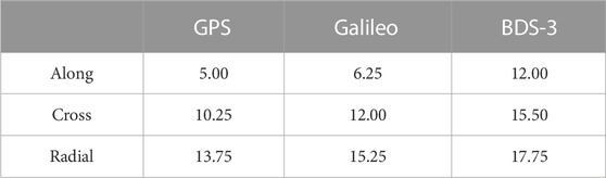
TABLE 2. Average convergence time in each direction for different satellite systems (unit: hour).

As shown in Figure 3, the SRIF orbit is rather stable after 48 h. Thus, the RMS of orbit difference after 48 h with respect to the WUM products can be taken as the final precision of the SRIF orbit. The orbit difference RMSs for each satellite after 48 h are shown in Figure 4. The average RMS for each system in different directions is also shown in the legend of the figure. It can be seen that the RMSs of most satellites in each direction are less than 0.1 m. The RMSs of GPS satellites are the best, while those of Galileo satellites are slightly larger. The RMSs of BDS-3 satellites are the largest among the three systems. To be specific, the average RMSs in the along-track, cross-track, and radial directions are 0.081 m, 0.046 m, and 0.029 m for GPS satellite, 0.079 m, 0.049 m, and 0.031 m for Galileo satellite, and 0.109 m, 0.066 m, and 0.054 m for BDS-3 satellite, respectively.

FIGURE 4

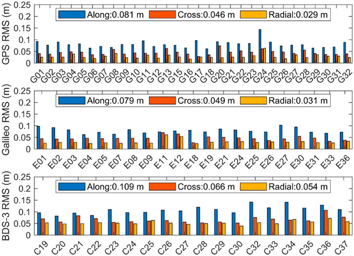
FIGURE 4. RMS of orbit differences with respect to the WUM products for each satellite after 48 h. The mean RMS for all satellites in each direction is shown.

3.2 Determination of the stochastic model of the constraint equation

Using Eq. 9, as discussed in Section 2, we compare the 24-h predicted part of ultra-rapid products released by WUM and the SRIF orbit after 48 h (stable SRIF orbit) with the WUM final orbit. The time series of RMS of the 24-h predicted orbit (blue dotted curve), the SRIF orbit (green dotted curve), and the difference between the 24-h predicted orbit and the stable SRIF orbit (red solid curve) for all satellites of each system are shown in Figure 5. Since the accuracy of SRIF orbit after 48 h basically remains stable, the statistical value shown in Figure 4 is adopted, and thus the green dotted curve is parallel to the horizontal axis.

FIGURE 5

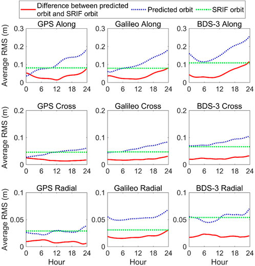
FIGURE 5. Time series of average RMS of the 24-h predicted orbit, the SRIF orbit after 48 h, and the difference between them for all satellites of each constellation.

As for the 24-h predicted orbit, the average RMS generally increases for GPS and Galileo satellites in the along-track and cross-track directions, as well as BDS-3 satellites in the cross-track direction. Due to the increase in the predicted time, the orbit error accumulates after orbit integration. Therefore, the predicted orbit tends to be less accurate along with the predicted time. Different from the along-track and cross-track directions, the variation trend of the average RMS of all systems in the radial direction generally remains flat for most time. In addition, the accuracy in the along-track direction of BDS-3 satellite increases in the first 6 h and then generally decreases. This is due to relatively larger discontinuity between the final products of two consecutive days than that of GPS and Galileo satellites.

From the red solid curve in Figure 5, we can find that the RMS of the orbit differences first decreases and then gradually increases for all satellites in the along-track direction, as well as GPS and Galileo satellites in the cross-track direction. This is because the accuracy of 24-h predicted part of the ultra-rapid orbit is better than that of the stable SRIF orbit in the beginning and then it is worse than that of the stable SRIF orbit as time goes on. It takes approximately 6–12 h to reach the bottom of the curve. In the cross-track direction for BDS-3 satellites, the accuracy of predicted orbit decreases with the increase in time and is always worse than that of the stable SRIF orbit. Therefore, the RMS of orbit differences keeps continuously increasing. In the radial direction of Galileo satellites, the RMS of orbit difference will first slightly decrease and then generally increase. On the contrary, there is no significant regularity of the RMS of orbit differences for GPS and BDS-3 satellites in the radial direction and it remains very stable.

The average values of the RMS of orbit difference between the predicted orbit and stable SRIF orbit from different predicted time length is shown in Table 3. It shows that the RMS of the difference over 6 h in the along-track, cross-track, and radial directions are 0.026/0.016/0.007 m for GPS satellite, 0.021/0.013/0.021 m for Galileo satellite, and 0.041/0.020/0.015 m for BDS-3 satellites, respectively. Generally speaking, the RMS of the difference over 12 h has the lowest value, while that over 24 h has the largest value in the along-track and cross-track directions. For the radial direction, the RMS of the orbit difference between different time ranges is generally the same except for Galileo and BDS-3 over 24 h. The values in the table are taken as a basis for the determination of the constant stochastic model of the constraint equation in our subsequent experiment.

TABLE 3

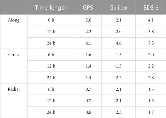
TABLE 3. Average RMS of the difference between the predicted orbit from ultra-rapid products and the stable SRIF orbit for all satellites (unit: cm).

If only the constant stochastic model is adopted, the value of the constraint may not adjust to the change in difference between the predicted orbit and the stable SRIF orbit over time. In order to build the time-dependent stochastic model of the constraint equation, the linear function, quadratic function, and cubic function related to the time $t$ is selected to fit the along-track, cross-track, and radial directions according to the time series pattern shown in Figure 5. The goodness of fit ($R^2$) of three different functions is listed in Table 4.

TABLE 4

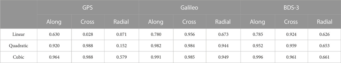
TABLE 4. Goodness of fit (${\mathit{R}}^{\mathbf{2}}$) of linear function, quadratic function, and cubic function to fit the RMS of the differences between the 24-h predicted ultra-rapid product and the stable SRIF.

From Table 4, we can find that the quadratic function greatly improves the fit performance of the linear function in all directions for GPS, Galileo, and BDS-3 satellites. For GPS and BDS-3 satellites, $R^2$ of the quadratic function in the along-track and cross-track directions exceeds 0.9. However, $R^2$ of the quadratic function in the radial direction is much lower, which are 0.152 and 0.653, respectively. This is because the RMS of the difference in radial direction of GPS is at the millimeter level, which is too small to be recognized as a clear regular trend of time-varying changes. For Galileo satellite, $R^2$ of all directions exceeds 0.9. This indicates that the quadratic function can fit the Galileo satellite well in all directions. Compared to the quadratic function, the cubic function mainly improves the radial direction for GPS satellite while the improvement in other directions for all navigation systems is limited. Although $R^2$ in the radial direction for GPS satellite is improved using the cubic function, there is no need to adopt the cubic function to model all satellites because the RMS of the difference changing over time in the radial direction for GPS is rather small. Therefore, the quadratic function is more suitable to build the time-dependent stochastic model of the constraint equation for GPS, Galileo, and BDS-3 satellites. The expression of the quadratic function is shown in Eq. 15, and the corresponding coefficient estimates are shown in Table 5.

${\sigma }_{Vx,RTN}=a\bullet t^2+b\bullet t+c.(15)$

TABLE 5

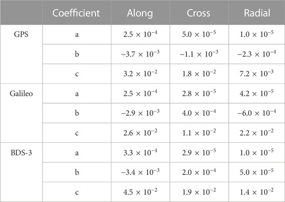
TABLE 5. Coefficient estimates of the quadratic function of the difference between the ultra-rapid product and stable SRIF orbit for each constellation.

The time series of fit residuals for each system in each direction are shown in Figure 6. It can be seen that the majority of residuals is in a range of −1 cm–1 cm, with an average value close to zero. The absolute values of residuals in the along-track direction are relatively larger than those in the cross-track and radial directions. The average RMSs of residuals in the along-track, cross-track, and radial directions are 5.8/0.6/1.1 mm for GPS satellite, 3.3/1.1/0.8 mm for Galileo satellite, and 7.5/1.4/1.4 mm for BDS-3 satellite, respectively. This indicates that the quadratic function can precisely fit the difference between ultra-rapid product and stable SRIF orbit.

FIGURE 6

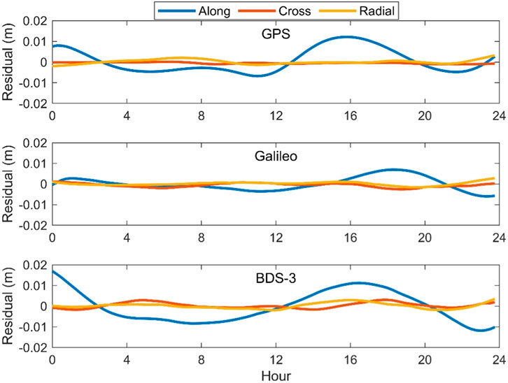
FIGURE 6. Fit residuals of the difference between 24-h predicted part of the ultra-rapid orbit and the stable SRIF orbit for all satellites of each constellation.

3.3 Real-time POD with external constraints from different schemes

The performance of real-time POD with external constraints is analyzed in this section. POD results with the constant stochastic model and the time-dependent stochastic model of the constraint equation are compared to those without external constraints. According to the average convergence time of each system (see Table 2), the constraint period in our experiment is chosen as 14 h, 16 h, and 18 h for GPS, Galileo, and BDS-3 satellites, respectively. Figure 5 shows that the accuracy of ultra-rapid products is better than that of the stable SRIF orbit in the first 6–12 h. Therefore, the ultra-rapid product is not suitable for the baseline of the constraint equation after 6–12 h if the constraint orbit is not updated timely. Considering that the ultra-rapid product is updated every 6 h, we choose to update the constraint orbit every 6 h during the constraint period in our scheme. Therefore, for the scheme with the time-dependent stochastic model, the argument of time $t$ in the quadratic function (see Eq. 15) will repeat every 6 h to determine the time-variant STD of the OMC of the constraint equation. For the scheme with the constant stochastic model, the RMS over 6 h and 24 h (see Table 3) is used as the constant STD of the OMC of the constraint equation, respectively. The time series of the RMS of orbit differences from different schemes with respect to the WUM orbit products are shown in Figure 7. The corresponding average RMS is shown in Figure 8, where the results during the constraint period is shown in the left panels and those after the constraint period is shown in the right panels. Note that the scope of the vertical axis in Figure 8 is limited to 0.5 m to clarify the results of the proposed method although some of the orange bars in the left panel exceed this scope.

FIGURE 7

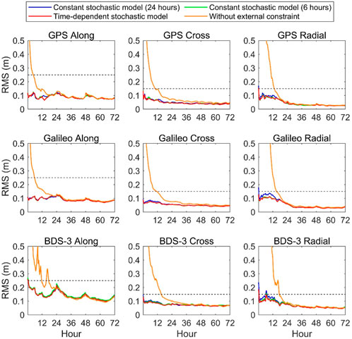
FIGURE 7. Time series of the RMS of differences between the SRIF orbit results and the WUM orbit products for different schemes.

FIGURE 8

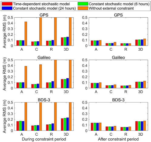
FIGURE 8. Average RMS of the orbit differences for different systems from three schemes.

Figure 7 shows that the convergence time of the schemes with external constraints in all directions is significantly reduced when compared with that of the schemes without external constraints. In the scheme with the constant stochastic model (24 h), there is no significant convergence phenomenon for GPS and Galileo satellites under the convergence criteria of 0.25 m, 0.15 m, and 0.15 m in the along-track, cross-track, and radial directions, respectively. However, there still exists a convergence phenomenon of less than 1 hour for BDS-3 in all directions. In the scheme with the constant stochastic model (6 h), no significant convergence phenomenon is observed for all systems in all directions. In the scheme with the time-dependent stochastic model, the RMS for GPS, Galileo, and BDS-3 satellites in all directions has a further improvement during the constraint period when compared to the scheme with the constant stochastic model (6 h). This indicates that different stochastic models of the constraint equation have a significant effect on the performance of convergence. In addition, the time-dependent stochastic model achieves more improvement in the cross-track and radial directions than the along-track direction for all systems when compared to the constant stochastic model.

The left panel of Figure 8 shows that the average RMSs in the along-track, cross-track, and radial directions are 0.092/0.072/0.086 m for GPS satellites, 0.099/0.068/0.099 m for Galileo satellites, and 0.164/0.087/0.106 m for BDS-3 satellites in the scheme with the time-dependent stochastic model, respectively. These values are almost at the same level as those after the constraint period shown in the right panel of the figure. Nevertheless, the RMSs in all directions for GPS, Galileo, and BDS-3 satellites all exceed 0.3 m in the scheme without external constraints. Compared to the average RMSs of the scheme without external constraints, the scheme with the constant stochastic model (6 h) during the constraint period shows an improvement of 86.5%, 84.8%, and 96.8% in the 1D direction for GPS, Galileo, and BDS-3 satellites. Compared with the scheme with the constant stochastic model (24 h), the scheme with the constant stochastic model (6 h) shows an improvement of 5.0%, 10.0%, and 4.8% in the 1D direction for GPS, Galileo, and BDS-3 satellites. Furthermore, the scheme with the time-dependent stochastic model performs better than the scheme with the constant stochastic model (6 h) with an improvement of 1.3% and 3.7% in 1D direction for GPS and BDS-3 satellites. For Galileo satellite, the average RMSs of the schemes with the time-dependent stochastic model and the constant stochastic model (6 h) are comparable. It demonstrates that the time-dependent stochastic model achieves a better performance than the constant stochastic model. After the constraint period, the right panel of the figure shows that the three schemes with external constraints basically perform with a comparable accuracy, which is slightly better than the scheme without external constraints. Therefore, our proposed constraint method can significantly improve the orbit accuracy in the convergence period without damaging the orbit accuracy after convergence.

Due to the limited manuscript space, the effectiveness and difference of the model results derived from different ACs and different satellite systems need further verification in the future research.

4 Discussion

The ultra-rapid orbit product is reliable external information to shorten the convergence time of the filter orbit because it can provide the predicted GNSS satellite orbit at the centimeter level. However, the problem of appropriately determining the stochastic model of the constraint equation derived from the ultra-rapid orbit has not been solved yet. In view of this, we propose an improved approach where the stochastic model is developed by analyzing the differences between the predicted part of the ultra-rapid orbit and the filter orbit after convergence. The constraint equation is added to the observation equation at every processing epoch to obtain an improved performance of the real-time orbit after the filter starts.

To validate the proposed method, 1-month data collected from 80 globally distributed IGS MGEX stations are processed using the SRIF method. The performance of the scheme without external constraints is first evaluated. Under the convergence criteria of 0.25 m, 0.15 m, and 0.15 m in the along-track, cross-track, and radial directions, the results show that the convergence time in the along-track, cross-track, and radial directions is 5.00/10.25/13.75 h for GPS satellite, 6.25/12.00/15.25 h for Galileo satellite, and 12.00/15.50/17.75 h for BDS-3 satellite, respectively. The average orbit accuracy after 48 h in the along-track, cross-track, and radial directions is 0.081/0.046/0.029 m for GPS satellite, 0.079/0.049/0.031 m for Galileo satellite, and 0.109/0.066/0.054 m for BDS-3 satellite. Afterward, we analyze the time series of the orbit differences between 24-h predicted part of the ultra-rapid orbit product and the stable SRIF orbit. The constant stochastic model is then determined by averaging the RMS of the orbit differences in different time ranges. Considering that the predicted orbit of the ultra-rapid products varies over time, a time-dependent stochastic model is also developed. The goodness of fit ($R^2$) of linear function, quadratic function, and cubic function is compared to determine the STD of the OMC of the constraint equation. Results show that the quadratic function is suitable to fit the difference between 24-h predicted part of the ultra-rapid orbit product and the stable SRIF orbit in all directions.

The experiments of different schemes with external constraints of the constant stochastic model and the time-dependent stochastic model are carried out. In the scheme with the constant stochastic model using average RMS values over 24 h, the results show that there is no convergence phenomenon in all directions for GPS and Galileo satellites under the same convergence criteria of the results without external constraints. However, there still exists a convergence phenomenon of less than an hour in all directions for BDS-3 satellites. In the scheme with the constant stochastic model using average RMS values over 6 h, no significant convergence phenomenon exists for all systems in all directions. When compared to the results without introducing external orbit constraints, the 1D RMS value during the constraint period is improved by 86.5%, 84.8%, and 96.8% for GPS, Galileo, and BDS-3 satellites. In the scheme with the time-dependent stochastic model, the accuracy during the constraint period shows a further improvement of 1.3% and 3.7% in the 1D direction for GPS and BDS-3 satellites when compared to that with the constant stochastic model using RMS values over 6 h, while the average RMSs of the two schemes are generally the same for Galileo satellite. After the constraint period, results with both the constant stochastic model and time-dependent model are at the same level, which is slightly better than those without external constraints. The aforementioned results indicate that our proposed method of using the ultra-rapid product as external constraints can significantly improve the convergence performance without damaging the orbit accuracy after convergence, and the constraint with the time-dependent stochastic model can further improve the convergence performance when compared to the constraint with the constant stochastic model.

Data availability statement

The datasets presented in this study can be found in online repositories. The names of the repository/repositories and accession number(s) can be found in the article/Supplementary Material.

Author contributions

LZ contributed to all the work and drafting of the article. LF and XF contributed to the technical route, designing of the research, and revising the article. ZL contributed to the analysis and interpretation of the experimental data. CS contributed to the interpretation of results. All authors listed have made a substantial, direct, and intellectual contribution to the work and approved it for publication.

Funding

This work was supported by the National Natural Science Foundation of China (Grant Nos 42274041 and 41931075).

Acknowledgments

The authors thank IGS for providing GNSS data and Wuhan University for providing ultra-rapid GNSS orbit products.

Conflict of interest

The authors declare that the research was conducted in the absence of any commercial or financial relationships that could be construed as a potential conflict of interest.

Publisher’s note

All claims expressed in this article are solely those of the authors and do not necessarily represent those of their affiliated organizations, or those of the publisher, the editors, and the reviewers. Any product that may be evaluated in this article, or claim that may be made by its manufacturer, is not guaranteed or endorsed by the publisher.

References

1. Arnold D, Meindl M, Beutler G, Dach R, Schaer S, Lutz S, et al. CODE’s new solar radiation pressure model for GNSS orbit determination. J Geodesy (2015) 89(8):775–91. doi:10.1007/s00190-015-0814-4

CrossRef Full Text | Google Scholar

2. Boehm J, Werl B, Schuh H. Troposphere mapping functions for GPS and very long baseline interferometry from European centre for medium-range weather forecasts operational analysis data. J Geophys Res Solid Earth (2006) 111:B02406. doi:10.1029/2005jb003629

CrossRef Full Text | Google Scholar

3. Dai X, Lou Y, Dai Z, Qing Y, Li M, Shi C. Real-time precise orbit determination for BDS satellites using the square root information filter. GPS Solutions (2019) 23(2):45–58. doi:10.1007/s10291-019-0827-1

CrossRef Full Text | Google Scholar

4. Duan B, Hugentobler U, Chen J, Selmke I, Wang J. Prediction versus real-time orbit determination for GNSS satellites. GPS Solutions (2019) 23(2):39–10. doi:10.1007/s10291-019-0834-2

CrossRef Full Text | Google Scholar

5. Fan L, Shi C, Beidou LM. Satellite real-time precise orbit determination using ultra-rapid ephemeris' constraint. J Geodesy Geodynamics (2018) 38(9):937–42. (in Chinese). doi:10.14075/j.jgg.2018.09.011

CrossRef Full Text | Google Scholar

6. Glocker M, Landau H, Leandro R, Nitschke M. Global precise multi-GNSS positioning with trimble centerpoint RTX. In: Proceedings of the 6th ESA workshop on satellite navigation technologies (navitec 2012) & European workshop on GNSS signals and signal processing (2012). p. 1–8. doi:10.1109/NAVITEC.2012.6423060

CrossRef Full Text | Google Scholar

7. Guo F, Li X, Zhang X, Wang J. Assessment of precise orbit and clock products for Galileo, BeiDou, and QZSS from IGS multi-GNSS experiment (MGEX). GPS Solutions (2017) 21(1):279–90. doi:10.1007/s10291-016-0523-3

CrossRef Full Text | Google Scholar

8. Kuang K, Li J, Zhang S. Galileo real-time orbit determination with multi-frequency raw observations. Adv Space Res (2021) 67(10):3147–55. doi:10.1016/j.asr.2021.02.009

CrossRef Full Text | Google Scholar

9. Leandro R, Santos M, Langley R. Analyzing GNSS data in precise point positioning software. GPS Solutions (2011) 15(1):1–13. doi:10.1007/s10291-010-0173-9

CrossRef Full Text | Google Scholar

10. Li R, Wang N, Li Z, Zhang Y, Wang Z, Ma H. Precise orbit determination of BDS-3 satellites using B1C and B2a dual-frequency measurements. GPS Solutions (2021) 25(3):95–14. doi:10.1007/s10291-021-01126-x

CrossRef Full Text | Google Scholar

11. Li X, Yuan Y, Zhu Y, Jiao W, Bian L, et al. Improving BDS-3 precise orbit determination for medium Earth orbit satellites. GPS Solutions (2020) 24(2):53–13. doi:10.1007/s10291-020-0967-3

CrossRef Full Text | Google Scholar

12. Li X, Zhu Y, Zheng K, Yuan Y, Liu G, Xiong Y. Precise orbit and clock products of Galileo, BDS and QZSS from MGEX since 2018: Comparison and PPP validation. Remote Sensing (2020) 12(9):1415. doi:10.3390/rs12091415

CrossRef Full Text | Google Scholar

13. Li Z, Li M, Shi C, Fan L, Liu Y, Song W, et al. Impact of ambiguity resolution with sequential constraints on real-time precise GPS satellite orbit determination. GPS Solutions (2019) 23(3):85–14. doi:10.1007/s10291-019-0878-3

CrossRef Full Text | Google Scholar

14. Lou Y, Liu Y, Shi C, Wang B, Yao X, Zheng F. Precise orbit determination of BeiDou constellation: Method comparison. GPS Solutions (2016) 20(2):259–68. doi:10.1007/s10291-014-0436-y

CrossRef Full Text | Google Scholar

15. Luzum B, Petit G. The IERS Conventions (2010): Reference systems and new models. Proc Int Astronomical Union (2012) 10(H16):227–8. doi:10.1007/s10291-014-0436-y

CrossRef Full Text | Google Scholar

16. Montenbruck O, Hauschild A, Steigenberger P. Differential code bias estimation using multi-GNSS observations and global ionosphere maps. Navigation (2014) 61(3):191–201. doi:10.1002/navi.64

CrossRef Full Text | Google Scholar

17. Montenbruck O, Steigenberger P, Prange L, Deng Z, Zhao Q, Perosanz F, et al. The multi-GNSS experiment (MGEX) of the international GNSS Service (IGS) – achievements, prospects and challenges. Adv Space Res (2017) 59(7):1671–97. doi:10.1016/j.asr.2017.01.011

CrossRef Full Text | Google Scholar

18. Muellerschoen R, Reichert A, Kuang D, Heflin M, Bertiger W, Bar-Sever Y. Orbit determination with NASA's high accuracy real-time global differential GPS system. Proc ION GPS (2001) 2294–303. Institute of Navigation, Salt Lake City, September 11-14.

Google Scholar

19. Qing Y, Lou Y, Liu Y, Dai X, Cai Y. Impact of the initial state on BDS real-time orbit determination filter convergence. Remote Sensing (2018) 10(1):111. doi:10.3390/rs10010111

CrossRef Full Text | Google Scholar

20. Ray J, Senior K. IGS/BIPM pilot project: GPS carrier phase for time/frequency transfer and timescale formation. Metrologia (2003) 40(3):270–88. doi:10.1088/0026-1394/403/307

CrossRef Full Text | Google Scholar

21. Rebischung P, Schmid R. IGS14/igs14.atx: A new framework for the IGS products. In: AGU fall meeting 2016 (2016).

Google Scholar

22. Rodriguez-Solano C, Hugentobler U, Steigenberger P, Lutz S. Impact of Earth radiation pressure on GPS position estimates. J Geodesy (2012) 86(5):309–17. doi:10.1007/s00190-011-0517-4

CrossRef Full Text | Google Scholar

23. Rodriguez-Solano C, Nitschke M, Zhang F, Weinbach U, Brandl M, Landau H. Trimble RTX precise orbit determination of Galileo satellites (2016). doi:10.13140/RG.2.1.2297.5606

CrossRef Full Text | Google Scholar

24. Springer T, Hugentobler U. IGS ultra rapid products for (Near-) real-time applications. Phys Chem Earth, A: Solid Earth Geodesy (2001) 26(6-8):623–8. doi:10.1016/S1464-1895(01)00111-9

CrossRef Full Text | Google Scholar

25. Tapley B, Schutz B, Born G. Statistical orbit determination. In: BD Tapley, BE Schutz, and GH Born, editors. Burlington: Academic Press (2004). p. xi–xv. doi:10.1016/b978-0-12683630-1/50019-9

CrossRef Full Text | Google Scholar

26. Zhang Q, Moore P, Hanley J, Martin S Auto-BAHN: Software for near real-time GPS orbit and clock computations. Adv Space Res (2007) 39(10):1531–8. doi:10.1016/j.asr.2007.02.062

CrossRef Full Text | Google Scholar

27. Zhang X, Li X, Li P. Review of GNSS PPP and its application. Acta Geodaet Cartograph Sin (2017) 46(10):1399–407. doi:10.11947/j.AGCS.2017.20170327

CrossRef Full Text | Google Scholar

28. Zumberge J, Heflin M, Jefferson D, Watkins M, Webb F. Precise point positioning for the efficient and Robust analysis of GPS data from large networks. J Geophys Res (1997) 102(B3):5005–17. doi:10.1029/96JB03860

CrossRef Full Text | Google Scholar