Effective rheology of immiscible two-phase flow in porous media consisting of random mixtures of grains having two types of wetting properties

1 Introduction

It was in 1827 that Ohm published his law stating that electrical current is proportional to the voltage drop across a conductor [1], meeting fierce resistance from the physics community in the beginning. Darcy arrived in 1856 at a similar law for single-phase flow in porous media, i.e., the volumetric flow rate is proportional to the pressure drop across the porous medium [2]. Both of these fundamental laws are examples of there being a linear relationship between current and driving force. In the case of the Darcy law, the derivation based on pore scale physics has been a challenge, see e.g., Whitaker’s derivation based on momentum transfer [3].

The Darcy law for single-phase flow through a porous sample is given as follows:

$Q=-\frac{AK}{\mu L}\mathrm{\Delta }P,(1)$

where Q is the volumetric flow rate along the axis of the cylindrical sample, ΔP is the pressure drop along it in the flow direction, A is the area of the sample orthogonal to the flow direction, K is the permeability of the sample, μ is the viscosity of the liquid, and L is the system length.

In 1936, the Darcy law (1) was generalized to the simultaneous flow of two immiscible liquids by Wyckoff and Botset by essentially splitting it into two [4].

$Q_w=-\frac{AK{k}_{rw}}{{\mu }_{w}L}\mathrm{\Delta }P,(2)$

$Q_n=-\frac{AK{k}_{rn}}{{\mu }_{n}L}\mathrm{\Delta }P,(3)$

where the subscripts w and n refer to the wetting properties of the two fluids with respect to the matrix; w refers to the more wetting fluid and n to the less wetting fluid. The idea behind this split is simple. The wetting fluid will see a pore space reduced by the presence of the other fluid, leading to a reduction in effective permeability for the wetting fluid. The reduction parameter is the wetting relative permeability k_rw. Completely analogously, the non-wetting fluid sees an effective reduction of the permeability by a factor k_rn, the non-wetting relative permeability. The split was given physical contents when Wyckoff and Botset assumed that the two relative permeabilities were functions of the wetting saturation S_w alone, the wetting saturation being the pore volume occupied by the wetting fluid divided by the total pore volume and assuming the fluids are incompressible. Barenblatt et al. [5] have later shown that this assumption is valid if there exists a local phase equilibrium between the fluids, a condition that is fulfilled only for slow flows. A further assumption built into Eqs 2, 3 is that there are no macroscopic saturation gradients present.

The total volumetric flow rate is given by the sum of the volumetric flow rates of each fluid as follows

$Q=Q_w+Q_n,(4)$

and as a consequence, the generalized Darcy Eqs 2, 3 predict the following expression:

$Q=-\frac{AK}{L}\left[\frac{k_{rw}}{{\mu }_w}+\frac{k_{rn}}{{\mu }_n}\right]\mathrm{\Delta }P,(5)$

that is, a total volumetric flow rate being proportional to the pressure drop.

Eqs 2, 3 assume that there are no macroscopic saturation gradients. If this is not the case, the pressure is split into one associated with the non-wetting fluid, P_n, and one associated with the wetting fluid, P_w. Their difference is equal to the capillary pressure function, P_n − P_w = P_c(S_w), which is also assumed to depend only on the S_w. Eqs 2, 3 will then contain terms of the type ∇P_c = (dP_c/dS_w)∇S_w, thus setting up the pressure gradient and the saturation gradient as driving forces. When these equations are combined with mass conservation, the result is a closed set of equations that determine how the saturation develops within the porous medium.

When the saturation changes inhomogeneously in the porous medium with time, one implicitly assumes that fluid interfaces move within the porous medium. It was then a surprise when Tallakstad et al. [6, 7] reported a flow rate Q depending on ΔP as follows:

$Q\propto |\mathrm{\Delta }P{|}^{\beta },(6)$

with β ≈ 1.85 for a two-dimensional glass-bead-filled Hele–Shaw cell filled with a water–glycerol mixture and air in the flow regime where the generalized Darcy Eqs 2, 3 are supposed to be valid. This study was followed up by an NMR study of the three-dimensional glass bead packings by Rassi et al. [8] finding an exponent β varying between 2.2 and 3.3. Aursjø et al. [9] using the same model porous medium as Tallakstad et al. [6, 7], but with two incompressible fluids, found β ≈ 1.5 or 1.35, depending on the fractional flow rates. Similar results, in the sense that β is considerably larger than one, have since been observed by a number of groups; see [10–13]. There has also been a considerable effort to understand these results theoretically and reproduce them numerically [6, 7, 14–25].

It should be pointed out that the power law behavior seen in Eq. 6 is different from that described by Wilkinson in 1986 [26]. In his work, Wilkinson used the invasion percolation model to work out the dependence of the relative permeabilities on the capillary pressure, which could be linked to the saturation. He found that the non-wetting relative permeability k_rn would depend on the difference between the capillary pressure P_c and a critical capillary pressure $P_c^c$ related to the percolation critical point, which is shown as follows:

$k_{rn}\sim {\left(P_c-P_c^c\right)}^t,(7)$

where t is the percolation conduction exponent [27]. This is, however, a very different problem from that giving rise to Eq. 6. The power law in (7) is a direct reflection of the geometry of the clusters of the non-wetting fluid in the system after the invasion process. Hence, it is a static problem. The power law in (6) is, as we shall see, the result of a dynamic process caused by the motion of the fluid interfaces.

The power law behavior in Eq. 6 is due to a competition between the capillary and the viscous forces. It is straightforward to understand why the flow rate should increase faster than linear when these forces are in competition. When the pressure difference across the porous medium is increased, more interfaces begin to move, leading to a higher effective permeability [28]. The reason why it should be a power law is less obvious. The best argument was perhaps already given by Tallakstad et al. [6, 7] through comparing the pressure drop across fluid clusters with the capillary pressures holding them in place. Capillary fiber bundle models [29, 30] are porous media in the form of bundles of capillary fibers, and they are typically simple enough to be mathematically solvable [16, 19–21, 24, 25]. When the fibers have undulating radii along the long axis, they show non-linear volumetric flow rate vs. pressure drop; they are not quite of the form (6) but rather

$Q=\left\{\begin{array}{cc}0\hfill & \text{if\hspace{0.17em}}|\mathrm{\Delta }P|\le P_t,\hfill \\ M{\left(|\mathrm{\Delta }P|-P_t\right)}^{\beta }\hfill & \text{if\hspace{0.17em}}{P}_t<|\mathrm{\Delta }P|<P_{\max },\hfill \\ M_D\left(|\mathrm{\Delta }P|-P_t\right)\hfill & \text{if\hspace{0.17em}}{P}_{\max }\ll |\mathrm{\Delta }P|,\hfill \end{array}\right.(8)$

where P_t is a threshold pressure necessary for the flow to occur, P_max is the maximum threshold pressure found in any capillary fiber, and M and M_D are mobilities. A non-zero threshold pressure is in general necessary in porous media when neither of the two immiscible fluids percolates when dealing with porous media and not just the capillary fiber bundle model [10, 15, 21]. The existence of a non-zero threshold pressure makes the measurement of β much harder than when it is zero as this implies determining two parameters simultaneously, (P_t, β), rather than just one, β.

A central unanswered question is whether the exponent β is universal in the sense that there are classes of systems that all have the same value, i.e., can one define universality classes? Intuitively, this is a very appealing idea as one has a diverging length scale, as in equilibrium critical phenomena as |ΔP| → P_t mentioned previously [6, 7]. The experimental measurements of β have so far neither given any indication of the existence of universality classes nor have the computational efforts due to the difficulties in dealing with two unknown parameters, P_t and β. Roy et al. [19] found using a capillary fiber bundle model that β = 2 if the fiber-to-fiber probability distribution of thresholds includes P_t = 0 with a finite probability; otherwise, β = 3/2. The fibers here had smoothly undulating radii along the flow direction. Lanza et al. [24] who studied a non-Newtonian mixture of immiscible Newtonian and non-Newtonian fluids in a capillary fiber bundle model found a different value of β when the radius distribution is jagged from when it is smooth.

Eq. 8, which was derived for the capillary fiber bundle model, predicts there being a pressure drop |ΔP| = P_t below which the flow rate Q is zero. This threshold may be zero. Within the capillary fiber bundle model, this means that some capillary tubes belonging to the bundle have interfaces that move as soon as there is a pressure difference across them. There is, however, one important mechanism missing in the capillary fiber bundle models: in the porous medium, the immiscible fluids may be percolating. In other words, there are pathways through the porous medium along which there are no interfaces. In this case, there will be a linear regime when the pressure drop is low enough so that the interfaces surrounding the percolating paths do not move. When the pressure drop is increased sufficiently for them to do so, the non-linear power law regime sets in.

Recently, Fyhn et al. [21] studied the exponent β and the threshold pressure P_t in a capillary fiber bundle model and a dynamic pore network model under mixed wet conditions. In the dynamic pore network model, each link was given a wetting angle—in the sense that if there is an interface in the link, this is the angle it will make with the walls of the tube—drawn from a given probability distribution. In the capillary fiber bundle model, each undulating tube is given a wetting angle from a given probability distribution. In both models, a constitutive law of the form (8) was found. The capillary fiber bundle model could be solved analytically, giving the following equation:

$\beta =\left\{\begin{array}{cc}1\hfill & \text{if\hspace{0.17em}}|\mathrm{\Delta }P|-P_t\gg P_{\max },\hfill \\ 2\hfill & \text{if\hspace{0.17em}}{P}_t\ll |\mathrm{\Delta }P|-P_t\ll P_{\max },\hfill \\ 3/2\hfill & \text{if\hspace{0.17em}}0<|\mathrm{\Delta }P|-P_t\ll P_t.\hfill \end{array}\right.(9)$

The network model studies showed a less clear picture, with β varying between 1 and 1.8, depending on the saturation and the wetting angle distribution. It was not possible to resolve whether there were regions of fixed β or whether it varied continuously with the parameters of the model. This was due to the non-zero threshold pressure P_t, which needed to be determined together with β.

We study here a model for immiscible two-phase flow in a porous medium made from two types of grains that have different wetting properties with respect to the fluids. The model treats the interfacial tension between the two fluids similarly to a model introduced by Irannezhad et al. [31, 32]. We imagine a packing of two types of grains, say type “+” and type “−.” Two immiscible fluids, denoted by “A” and “B,” flow through the pores between the grains denoted by “+” or “−”. Fluid “A” is fully wetting, and “B” is fully non-wetting with respect to “+” grains, whereas it is the opposite with respect to “−” grains. The direction of the capillary forces in the links between two “+” grains is, therefore, opposite compared to the direction in the links between two “−” grains, whereas the capillary forces in the links between two opposite types of grains are zero.

The probability that a grain is of “+” type is p⁺. A second parameter is the wetting saturation S_w. There is a rich phase diagram when plotting the threshold pressure P_t as a function of the two control variables p⁺ and S_w, which is illustrated in Figure 1. It should be noted, in particular, in this phase diagram that there is a region in the middle where the threshold pressure P_t = 0. This region is limited by two p⁺ = constant critical lines. Each line signifies a percolation transition [27]. The two curved gray lines signify a possible shift of the two blue transition lines due to the dynamics of the model. There are also two other lines: one green line marked “hysteretic transition” and one red line marked “non-hysteretic” transition. Crossing such a line, one of the two fluids stops moving and we are essentially dealing with a single-phase flow problem. When the wetting fluid stops moving, there is no hysteresis. On the other hand, when the non-wetting fluid stops, there is hysteresis in the sense that wetting saturation has to be lowered more to get the non-wetting fluids moving again [33].

FIGURE 1

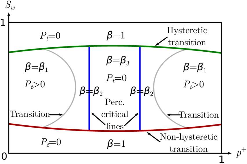
FIGURE 1. Phase diagram showing the exponent β and the threshold pressure P_t plotted against the occupation probability p⁺ and the saturation S_w. The diagram is symmetric about the p⁺ = 1/2 line. The two vertical blue lines are critical lines associated with the two percolation transitions. The lower red line is separating the two-phase flow from the single-phase flow. There is no hysteresis associated with this line. The upper green line also distinguishes between two-phase and single-phase flows. However, in this case, there is hysteresis. The two gray lines represent the transition lines from threshold pressure P_t = 0 to a non-zero value. The nature of these lines is unknown.

In the region where P_t = 0, while still having two-phase flow, we observe an exponent β = β₃ = 2.56 ± 0.05 for saturation S_w = 0.5. This value is also seen when setting p⁺ = p_c or p⁺ = 1 − p_c, where p_c ≈ 0.5927 is the site percolation threshold for square lattices, i.e., β = β₂ = β₃. For p⁺ much lower than 1 − p_c or p⁺ much higher than p_c, still for saturation S_w = 0.5, we see β = β₁ = 2.25 ± 0.1. The large uncertainty in β seen here stems from P_t > 0.

It is surprising that β₂ = β₃ within the precision we are able to obtain. The exponent β₂ is obtained at the percolation threshold where the paths where fluid surfaces meet no resistance are fractal with fractal dimension 4/3 as they are the external perimeters of percolation clusters [34]. The reason for not seeing the critical behavior reflected in β comes from there also being other links that have no interfacial tension in them as they contain no interfaces, thus driving the system away from criticality. In order to investigate whether there are any traces at all in the transport properties of the percolation critical point, we have studied the mobility M at low pressure drops as p⁺ approaches a critical value, where we expect it to vanish with an exponent t′ of the same type as the conductivity exponent t in ordinary percolation in the vicinity of the critical p⁺ [27, 35]. We find that t′ ≈ 5.7, indicating that the system is not critical and M falls off faster than algebraic. We, therefore, expect there to be two extra transition lines (marked in gray in Figure 1) that distinguish between P_t = 0 and P_t > 0. The nature of these lines is unknown.

We use a dynamic pore network model [36–40] for this study. It has been used earlier in the context of modeling-mixed wetting porous media; see [21, 41, 42]. We describe the model in Section 2 including our use of the wetting model similar to that introduced by Irannezhad et al. [31, 32]. Section 3 explains how we identify the paths through the network that have no capillary forces associated with them and relate them to a site percolation problem. Section 4 presents the analysis of the low pressure drop mobility at the percolation critical points. Section 5 constitutes our investigation of the volumetric flow rate Q vs. pressure drop ΔP. We fix the saturation S_w = 0.5 and scan through this line in the phase diagram in Figure 1 for different values of p⁺. We also tested whether there would be hysteresis with respect to increasing or decreasing the pressure drop, finding none. Section 6 contains a summary and our conclusions.

2 Dynamic pore network model

A sketch of the dynamic pore network (DPN) model used in this work is given in Figure 2, showing a square two-dimensional network with links with the same length tilted 45° from the flow direction. ΔP across the network drives the flow leading to Q, which is measured over a cross section of the system normal to the direction of the overall flow. The zoomed-in sketch to the right in Figure 2 illustrates the rules for using the wetting properties of the grains to assign wetting angles θ to the links, where θ is consistently defined through one of the fluids. In contrast to earlier models [21, 41, 42] that assign the wetting angles to the pores or links directly, the physical basis for this model is a mixture of grains and the wettability of the pore space in-between depends on the wettability of the surrounding grains, similar to the system introduced by Irannezhad et al. [31, 32]. We assume two types of grains, they being either fully non-wetting with θ = 180° or fully wetting with θ = 0°. Having fully non-wetting or fully wetting grains maximizes the difference between the two types of grains in terms of their wettability and, hence, maximizes any impact on the rheology that comes as a result of this difference. The grains are denoted fully non-wetting and assigned a notation “+” with an occupation probability p⁺, and the rest of the grains are then fully wetting with a notation “−”. For each link, θ is determined based on the link’s adjacent grains. Each grain in the network is connected to four links, which means each link has two adjacent grains, as shown in Figure 2. If both of the adjacent grains are assigned “+”, the link will have θ = 180°. If both of the adjacent grains are assigned “−”, then θ = 0°. Lastly, if one of the adjacent grains is “+” and the other one is “−”, the link in the middle should be easy to pass through for both fluids, and the wettability should be neutral with θ = 90°.

FIGURE 2

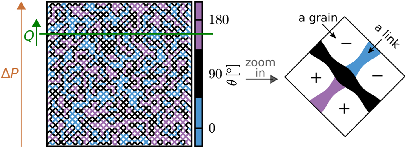
FIGURE 2. Dynamic pore network model implemented on a square lattice consists of links oriented 45° from the overall flow direction. The flow is driven by a global applied pressure ΔP, and the total volumetric flow rate Q is measured over a cross section normal to the direction of the overall flow. The wetting angle θ of each link is based on its adjacent grains. The grains are assigned “+” with an occupation probability p⁺, and the rest of the grains are assigned “−”. If both of the adjacent grains are assigned “+”, θ = 180° (marked pink). If both of the adjacent grains are assigned “−”, θ = 0° (marked blue). Lastly, if one of the adjacent grains is “+” and the other one is “−”, then θ = 90° (marked black), and hence, there are no capillary forces associated with interfaces in the link.

The networks have periodic boundary conditions in both directions. Two fluids that flow through the network are immiscible, and their movement is traced through the position of their interfaces at each instant in time. Whenever the fluids flowing in a link reach the crossing point with the three other links, namely, a node, the fluids get distributed into the neighboring links in the same time step instead of being retained in the node itself [36].

The volumetric flow in each link with length l, pointing along the link’s center axis x, is given by the following equation:

$q=-\frac{\pi {\bar{r}}^4}{8\mu l}\left(\mathrm{\Delta }p-\widehat{x}\cdot \left(\sum _k{p}_t\left(x_k\right){\widehat{J}}_k\right)\right),(10)$

where it has been assumed that the radius does not deviate too much from its average value $\bar{r}$ [36]. Here, μ = s_Aμ_A + s_Bμ_B is the saturation weighted viscosity of the fluids, where s_A and s_B are saturations of the two fluids A and B, respectively, with viscosities μ_A and μ_B in the links (in contrast to S_w, which is the average saturation over the whole network). Figure 3 can be used to further explain the variables in Eq. 10. The unit vector $\widehat{J}$ lies along the x-axis and points in the direction out of the fluid within which θ is defined. In Figure 3, θ is consistently measured through fluid A in both examples (a) and (b), regardless of if fluid A is more or less wetting with respect to the solid. Hence, $\widehat{J}$ also consistently points across the interface starting from fluid A toward fluid B. The sum in Eq. 10 is taken over the interfaces numbered k with varying ${\widehat{J}}_k$ with positions x_k ∈ [0, l] along x. The dot product of this sum with the unit vector $\widehat{x}$ in the positive x direction is taken afterward to obtain the total capillary pressure. The capillary pressure across one interface at position x which has an angle θ with the solid through fluid A is modeled by using the Young–Laplace equation [43],

$p_t\left(x\right)=\frac{2\sigma \cos \theta }{r\left(x\right)},(11)$

where σ is the surface tension and

$r\left(x\right)=\frac{r_0}{1-a\cos \left(\frac{2\pi x}{l}\right)}(12)$

is the radius where a is the amplitude of the periodic variation, and r₀/a is randomly chosen from the interval [0.1l, 0.4l]. This way, p_t varies with both the position along a link and from link to link.

FIGURE 3

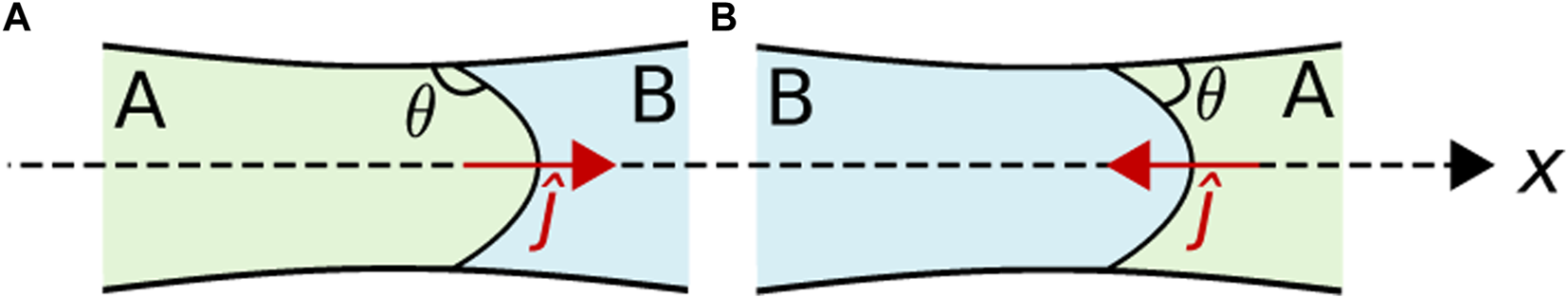
FIGURE 3. Wetting angle θ is consistently measured through fluid A in both examples (A,B), regardless of the wettability situation. The unit vector $\widehat{J}$ lies along the center axis x and points in the direction out of the fluid within which θ is measured, which, in this case, is from fluid A to fluid B.

For all simulations in the following, the two immiscible fluids have been given surface tension 3.0 ⋅ 10^–5 N/mm and viscosity 0.1 Pa⋅s for both. The overall network saturation is kept constant at 0.5, meaning there are equal amounts of the two fluids. The links in the network have length l = 1 mm. In all the figures, the logarithms are in base 10.

3 Easy links and connected paths

There are three types of links in the model: those that are of the “++” type, those that are of the “−−” type, and the “+−” = “ − +” type. We will, in the following, refer to the latter type as “easy links” since they offer no capillary resistance to interfaces that happen to be in them. Paths of connected easy links may percolate, i.e., stretch across the network forming loops as we are implementing bi-periodic boundary conditions. We will refer to such percolating paths of easy links as “connected paths”; see Figure 4.

FIGURE 4

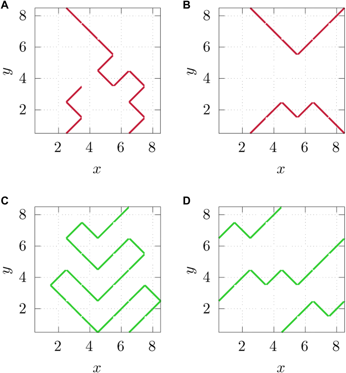
FIGURE 4. Due to periodic boundary conditions in both directions parallel and orthogonal to Q, it is not enough for a path to connect the bottom to the top of the network in the direction of Q to qualify as a connected path; it also has to loop back to itself. We show here four examples of clusters of easy links in an 8 × 8 lattice. Figures (A,B) do not qualify as connected paths, as defined for the networks in this work, while (C,D) do. The cluster of easy links in (A) connects the top and the bottom of the network but needs one additional link centered at (x, y) = (4, 4) to form a connected path. The cluster of easy links in (B) forms a closed loop but does not cross the network fully in the flow direction, which is along the y-axis. In (C), the link centered at position (x, y) = (1, 7) meets the link centered at (x, y) = (6, 8) due to the periodic boundary condition in the y-direction and completes the loop, hence making the path a connected path. The effect of having a periodic boundary condition in the x-direction is apparent in (D), where the link centered at (x, y) = (8, 2) connects to the link at (x, y) = (1, 3), and similarly, (x, y) = (8, 6) connects to (x, y) = (1, 7) and (x, y) = (4, 8) connects to (x, y) = (5, 1), thus completing the loop.

The geometry of the easy links and connected paths may be mapped onto an ordinary site percolation problem [27]. The links altogether form a square lattice. The nodes of the dual lattice form another square lattice [44] and are assigned “+” or “−”. These values are placed at random. The distribution of neighboring “+” sites in this dual lattice forms an ordinary site percolation problem. In an infinitely large lattice, there will be a percolating “+” cluster when p⁺ ≥ p_c, where p_c is the site percolation threshold 0.5927…. If we, on the other hand, focus on the “−” sites, there will be a cluster of such sites that percolate if p⁻ = 1 − p⁺ ≥ p_c or p⁺ ≤ 1 − p_c ≈ 0.4073… [45]. Hence, if 0 ≤ p⁺ ≤ 1 − p_c, the “−” clusters percolate, if 1 − p_c ≤ p⁺ ≤ p_c, neither the “−” sites nor the “+” sites percolate, and if p_c ≤ p⁺, the “+” sites percolate. We show in Figure 5 a map of the wetting angles associated with different values of p⁺. The easy links are shown in black.

FIGURE 5

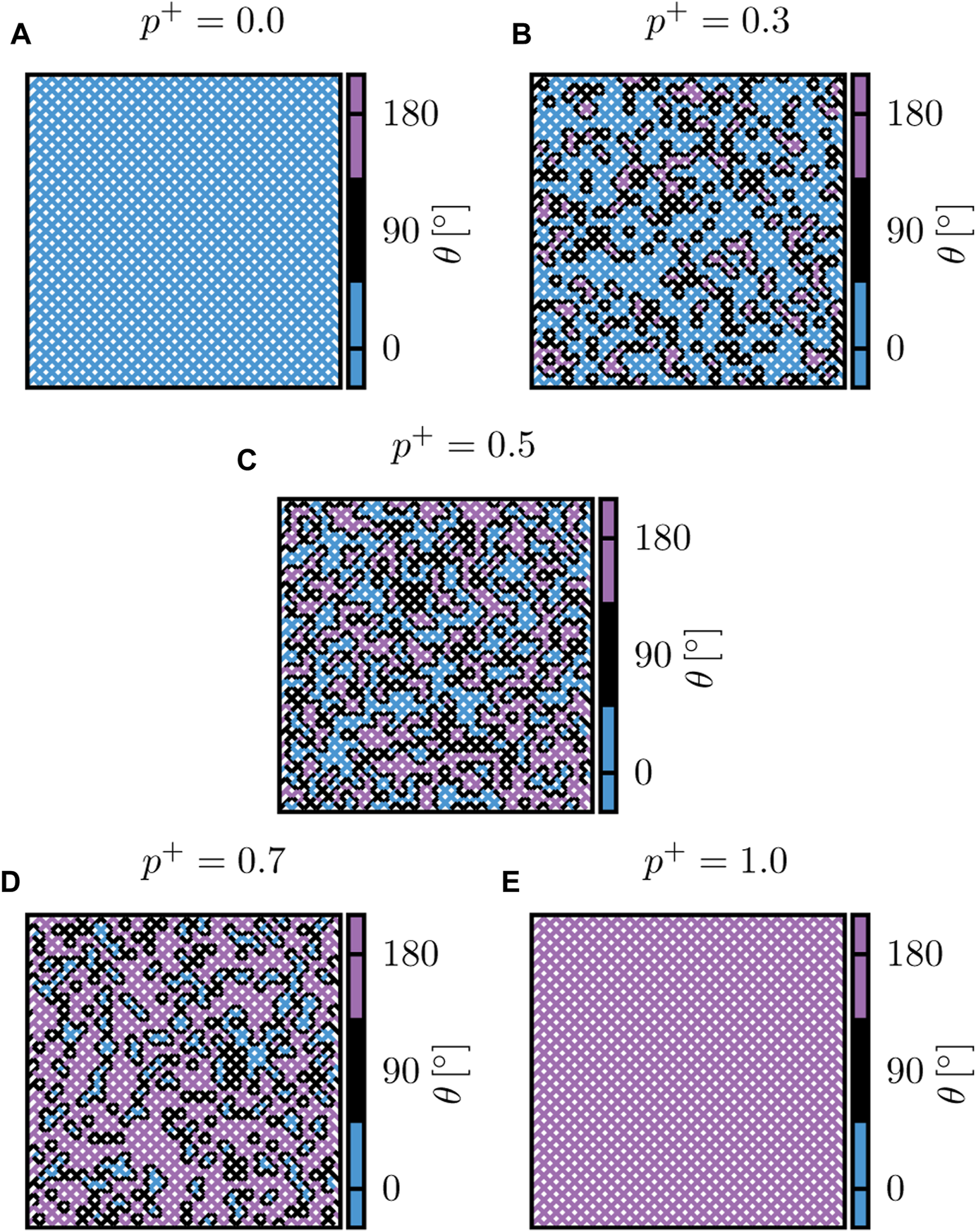
FIGURE 5. At p⁺ = 0, shown in (A), all the grains are fully wetting grains that are noted as “−” in Figure 2. This means that the pore space between these grains, namely, the links in DPN, all have θ = 0°. Oppositely at p⁺ = 1.0, shown in (E), there are only links that have θ = 180°. In these two extreme cases, there is no easy link in the network with neutral wettability θ = 90°. Moving away from these extremes, when p⁺ = 0.3 in (B) or when p⁺ = 0.7 in (D), links with θ = 90° are present but not enough to create a connected path that crosses the entire system. At the middle point of p⁺ = 0.5 (C), DPN has half of each type of grain, creating the highest possible probability for having connected paths with only θ = 90° links. In these examples, p⁺ = 0.5 (C) is the only one that lies within the limit 1− p_c < p⁺ < p_c, and it is only here we find connected paths.

We note that if neither the “+” sites nor the “−” sites percolate (1 − p_c ≤ p⁺ ≤ p_c), there must be connected paths. We, furthermore, note that if either of the two site types percolates, there cannot be any connected paths. At the two thresholds, p⁺ = 1 − p_c and p⁺ = p_c, the connected paths appear together with the appearance of a percolating cluster of either “−” or “+” type as the perimeter of the incipient percolating cluster is a connected path. At the percolation thresholds, we know that the fractal dimension of the perimeter, and hence the corresponding connected path, is 4/3 [34]. For values away from the critical points, the connected paths are not fractal. Hence, the structure of the easy link clusters and the connected path is very different away from the critical points while still being in the interval 1 − p_c ≤ p⁺ ≤ p_c.

The probability of finding a connected path as a function of p⁺ is investigated by testing 1,000 randomly generated networks with size L × L for each p⁺ ∈ {0.3000, 0.3001, 0.3002, …, 0.7000}. The results are shown in Figure 6 for L = 50 links and L = 100 links. We see that the two curves cross very close to 1 − p_c and p_c.

FIGURE 6

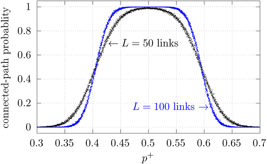
FIGURE 6. Probability for having connected paths in systems with non-wetting grain probability p⁺ and size L × L, where L is either 50 or 100 links.

4 Mobility

As we will show with the results presented in the following section, the constitutive law between the volumetric flow rate Q and the pressure drop |ΔP| can be written as follows:

$Q=\left\{\begin{array}{cc}M|\mathrm{\Delta }P|\hfill & \text{if\hspace{0.17em}}|\mathrm{\Delta }P|<P_l,\hfill \\ M_m|\mathrm{\Delta }P{|}^{{\beta }_3}\hfill & \text{if\hspace{0.17em}}{P}_l<|\mathrm{\Delta }P|<P_u,\hfill \\ M_D|\mathrm{\Delta }P|\hfill & \text{if\hspace{0.17em}}{P}_u<|\mathrm{\Delta }P|,\hfill \end{array}\right.(13)$

in the region 1 − p_c ≤ p⁺ ≤ p_c. Here, P_l and P_u are two crossover pressures. There are three regimes: 1) a linear regime for low pressure drops, 2) a non-linear regime for intermediate pressure drops, and 3) a linear regime for high pressure drops. Each regime is characterized by a mobility, M(p⁺, S_w), M_m(p⁺, S_w), and M_D(p⁺, S_w), respectively.

If we move to values of p⁺ where P_t > 0, regime (1) disappears. Hence, we have that M(p⁺, S_w) tends to zero as p⁺ reaches the boundary between the P_t = 0 region and the P_t > 0 region. We hypothesize, in the following, that the boundaries of this region are given by the percolation thresholds 1 − p_c and p_c.

Expecting that M(p⁺, S_w) shows similar behavior to the conductivity in percolation [35], we make the assumption that the mobility vanishes as

$M\sim \left\{\begin{array}{cc}{\left(p^{+}-\left(1-p_c\right)\right)}^{t^{\prime }}\hfill & \text{for\hspace{0.17em}}{p}^{+}\to {\left(1-p_c\right)}^{+},\hfill \\ {\left(p_c-p^{+}\right)}^{t^{\prime }}\hfill & \text{for\hspace{0.17em}}{p}^{+}\to {\left(p_c\right)}^{-},\hfill \end{array}\right.(14)$

where t′ is a transport exponent of the same type as the conductivity exponent t in ordinary percolation, which is 1.303(8) according to [46]. In Eq. 14, $p^{+}\to {(1-p_c)}^{+}$ means p⁺ approaches 1 − p_c from above and $p^{+}\to {(p_c)}^{-}$ means p⁺ approaches p_c from below. By using finite size scaling analysis, we obtain the following equation:

$M\sim L^{-t^{\prime }/\nu },(15)$

where ν is the correlation length exponent in percolation, which is known to be 4/3 [47].

To investigate the relation given in Eq. 15, we set p⁺ = 0.5927 ≈ p_c and network-dimensions L × L for L between 50 and 90 links. The lowest numerically feasible |ΔP| is used in order to stay in the lower linear regime in Eq. 13, specifically 2.8 Pa/link ⪅|ΔP|/L⪅5.8 Pa/link. When operating at low |ΔP|, the flow, which is mainly through the connected paths, stabilizes quickly and retains approximately a constant value compared to the fluctuating flow at higher |ΔP|. For these simulations, the flow is driven for approximately 40 pore volumes of fluid through the network, where one pore volume is equal to the total volume of the pore space in the network. The values of Q are calculated by averaging over the last 20 pore volumes simulated. Variation in the connected paths a network can have is covered by averaging the results over 50 network realizations. The results are shown in Figure 7, where we get t′/ν = 4.3 ± 1.0, giving the following equation:

$t^{\prime }=5.7\pm 1.3.(16)$

FIGURE 7

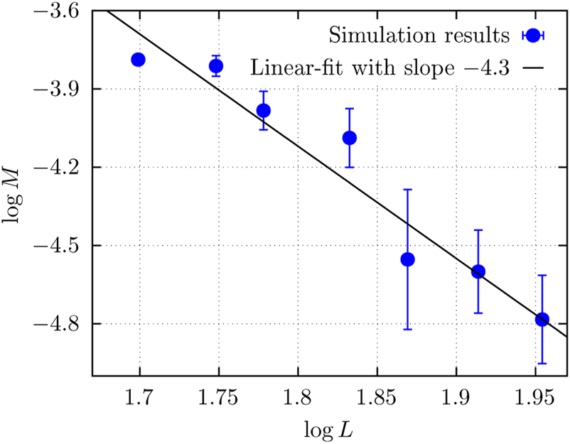
FIGURE 7. Mobility M in networks with size L × L. The slope of the linear fit is −t′/ν = −4.3 ± 1.0. The saturation was set to S_w = 0.5 in this calculation.

This is a huge value. A possible explanation for the observed value is that the system is not at a critical point in spite of the geometry of the easy links and the connected paths indicating this. In our argumentation, we have not taken into account the empty links, i.e., those links that do not contain any interfaces. They will be indistinguishable from the easy links with respect to the dynamics. These empty links drive the system away from the percolation critical point, and Figure 7 is in reality, indicative of non-algebraic behavior. We have indicated this possible shift in transition in the phase diagram shown in Figure 1.

5 Non-Darcy behavior

In the simulations performed for this section, networks have dimensions 100 × 100 links². For each |ΔP|, the flow is driven for approximately 100 pore volumes of fluid through the network. This ensures the steady-state flow, and the value of Q in the steady state is calculated by averaging over the total flow rate during approximately the last 25 pore volumes simulated.

5.1 Hysteresis

We pose, here, the question of whether there are any hysteretic effects from raising and lowering the pressure drop |ΔP| on the volumetric flow rate Q. The result is shown in Figure 8. With the passing of time, measuring in terms of injected pore volumes, |ΔP| applied across a network is raised and then lowered in steps. The |ΔP| values used, 200 Pa, 266 Pa, 355 Pa, 473 Pa, and 631 Pa, are from the lowest numerically feasible range. It can be observed from Figure 8 that whenever |ΔP| is returned to the same value, Q also quickly stabilizes back to the previous value it had with the same |ΔP|. This shows that the steady-state results generated using the DPN model do not depend on long-term memory [48].

FIGURE 8

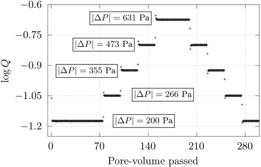
FIGURE 8. Increasing global pressure difference |ΔP| with the injected pore volumes raises the volumetric flow rate Q, and subsequently decreasing |ΔP| returns Q to the original value. Q was measured in units mm³/s.

5.2 Volumetric flow rate dependence on pressure drop

The results relating Q and |ΔP| in systems with zero P_t and different values of p⁺ are shown in Figure 9. We used p⁺ ∈ {0.42, 0.46, 0.50, 0.54, 0.58, and 0.5927} for the simulations. For each of these p⁺ values, the results were averaged over 10 randomly chosen networks that have connected paths, meaning 10 networks were randomly chosen from a subset of networks with zero threshold pressure P_t. To assist the understanding of Figure 9, velocity maps of a network with p⁺ = 0.5 at various |ΔP| have been plotted in Figure 10. The velocity maps show the steady-state averaged absolute velocities; in other words, they show the average speed of the fluid. The velocities are color coded so that those through neutral links with θ = 90° are in shades of red, and the rest that are through links with θ ∈ {0°, 180°} are in shades of blue. The results in Figures 9, 10 show three regimes in terms of β, as indicated in Eq. 13.

FIGURE 9

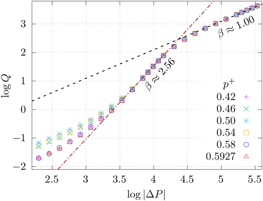
FIGURE 9. Total volumetric flow rate Q as a function of global pressure difference |ΔP| in systems with different non-wetting grain occupation probabilities p⁺. The results of linear fit with slopes β are included in the plot, where β is the exponent in Q ∝ |ΔP|^β. Q was measured in units mm³/s, and |ΔP| was measured in units Pa. This figure is the basis for Eq. 13.

FIGURE 10

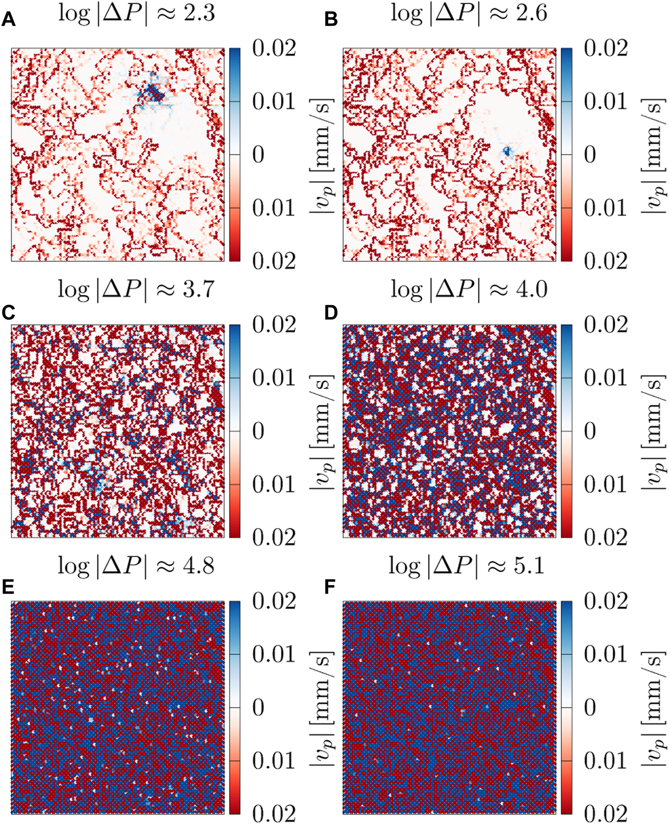
FIGURE 10. Maps of steady-state averaged absolute velocities |v_p| at different global pressure differences |ΔP|, where velocities through links with the wetting angle θ = 90° have shades of red and those through links with θ ∈ {0°, 180°} have shades of blue. The network had non-wetting grain occupation probability p⁺ = 0.5. |ΔP| was measured in units Pa.

The lowest regime in Eq. 13 seems to correspond to log  |ΔP|⪅2.8 in Figure 9; in other words, |ΔP|/L⪅6.3 Pa/link. The transition from this regime to the next is more gradual for p⁺ away from 0.5 in Figure 9. In this regime with very low |ΔP|, we find β = 1.00 ± 0.01. The velocity maps of a network with p⁺ = 0.5 at two different |ΔP| in this regime are shown in Figures 10A,B, and they indicate that the flow is mainly through the neutrally wet (red) links. When increasing log  |ΔP| from Figure 10A to Figure 10B, the impact mainly manifests in the increase of the speed of the fluids rather than the creation of new paths. Therefore, it makes sense that the flow remains Darcy-like with β approximately equal to 1. In the lowest regime in Figure 9, it is apparent that the mobility M in Eq. 13 decreases when p⁺ moves away from 0.5 toward p_c ≈ 0.5927 and 1 − p_c ≈ 0.4073. In this regime, the flow is mainly through the connected paths. The network has more connected-path links and transports more fluid for the same |ΔP| value, hence resulting in a larger Q value, meaning a larger M value when p⁺ moves toward 0.5. For instance, at log  |ΔP| ≈ 2.3, the number of active connected-path links is high at p⁺ = 0.5, as can be seen in Figure 10A, slightly lower at p⁺ = 0.54, as can be seen in Figure 11A, and significantly lower at p⁺ = 0.58, as can be seen in Figure 11B, making Q at p⁺ = 0.58 significantly less than in the other two cases.

FIGURE 11

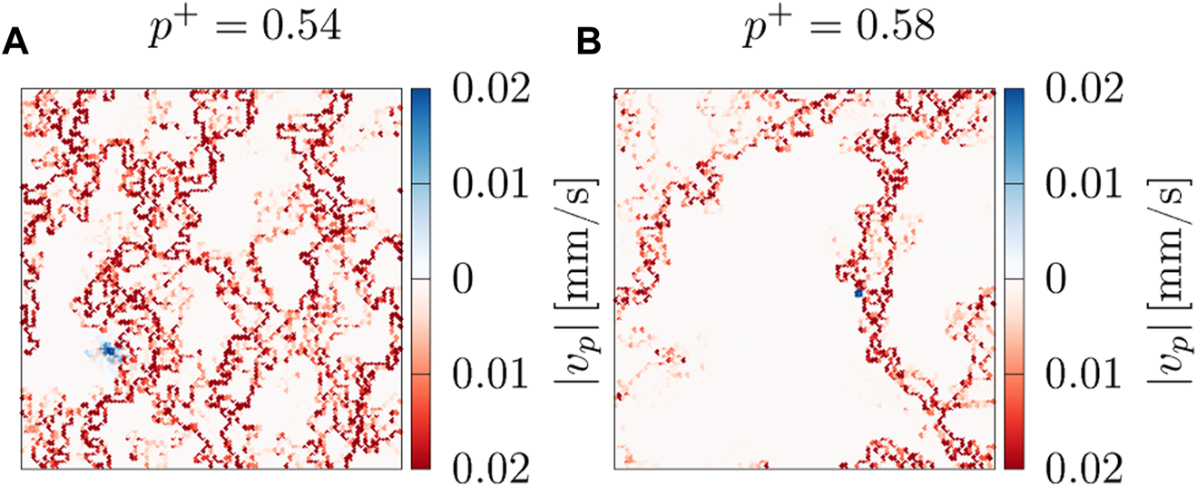
FIGURE 11. Maps of steady-state averaged absolute velocities |v_p| at log  |ΔP| ≈ 2.3, where |ΔP| is the global pressure difference. The velocities through links with the wetting angle θ = 90° have shades of red, and those through links with θ ∈ {0°, 180°} have shades of blue. p⁺ is the non-wetting grain occupation probability.

The middle regime in Eq. 13 seems to correspond to 3.3⪅ log  |ΔP|⪅4.1 in Figure 9; in other words, 20.0 Pa/Link ⪅|ΔP|/L⪅125.9 Pa/link. Here, the exponent in Eq. 13 is β = β₃ = 2.56 ± 0.05, and M_m is the same for all p⁺ values examined. When log  |ΔP| increases from Figure 10C to Figure 10D in this regime, the velocity maps show that there is a significant increase in the number of flow carrying links, meaning Q also increases significantly. The opening of new paths in addition to the increased flow in the already active paths explains β being large. At this level of |ΔP|, M_m and β being the same for all p⁺ examined makes sense as the connected paths that differentiate networks with different p⁺ no longer are the main contributors to the flow.

The highest regime in Eq. 13 seems to correspond to log  |ΔP|⪆4.5 in Figure 9; in other words, |ΔP|/L⪆316.2 Pa/link. Here, the exponent in Eq. 13 is β = 1.00 ± 0.01, and M_D is the same for all p⁺ examined. The velocity maps taken from two different points in this regime are shown in Figures 10E,F. In both cases, almost all the links in the network are carrying flow, regardless of their wettability; hence, increasing |ΔP| does not create new paths. The effect of capillary barriers in the links becomes insignificant in comparison to the enormous pressure drop across the links, making all p⁺ produce the same Q at the same |ΔP|. Increasing |ΔP| in this regime increases Q linearly, which is indicative of Darcy flow.

As the results in Section 3 show, there are very few to zero connected paths outside of the range 1 − p_c ≤ p⁺ ≤ p_c examined in Figure 9. If p⁺ was very close to the range examined in Figure 9, the behavior of β and M would have been expected to be the same as in Figure 9 since the flow will similarly be carried by the connected paths. To test p⁺ further away, simulations have been performed with p⁺ = 0.2 and 0.3, and the results are shown in Figure 12. Here, P_t is not zero, unlike the systems used for Figure 9 and corresponding constitutive Eq. 13. In this case, we find a constitutive equation

$Q=\left\{\begin{array}{cc}0\hfill & \text{if\hspace{0.17em}}|\mathrm{\Delta }P|\le P_t,\hfill \\ M_m{\left(|\mathrm{\Delta }P|-P_t\right)}^{\beta }\hfill & \text{if\hspace{0.17em}}{P}_t<|\mathrm{\Delta }P|<P_u,\hfill \\ M_D\left(|\mathrm{\Delta }P|-P_t\right)\hfill & \text{if\hspace{0.17em}}|\mathrm{\Delta }P|<P_u,\hfill \end{array}\right.(17)$

where P_u is the crossover pressure between non-linear and Darcy behavior. By varying P_t from 0.00 Pa to the lowest |ΔP| in the datasets with an increment of 0.01 Pa, mathematical linear fits with slopes β were calculated at the lowest pressures to find the candidate that gave the least root-mean-square error. This gave β = 2.23 ± 0.05 and $P_t=\left(3.4\pm 0.5\right)$ kPa for p⁺ = 0.2, and β = 2.29 ± 0.05 and $P_t=\left(2.0\pm 0.5\right)$ kPa for p⁺ = 0.3. The regime these β correspond to is the middle regime discussed in Figure 9, where the behavior was also non-linear due to the capillary barriers created by the interfaces between the two fluids. Fyhn et al. [21] have observed β > 1 behavior even in networks with the same wetting angle everywhere, which would be the same as having p⁺ → 0.0 or 1.0 here. Due to the lack of connected paths in systems with p⁺ = 0.2 and 0.3, the lowest regime in Figure 9 does not appear for the results in Figure 12. Lastly, the highest regime where β ≈ 1 should occur for all where the flow pushes through almost the entire network and there is almost no influence of p⁺. This is indeed what we see in Figure 12 as well.

FIGURE 12

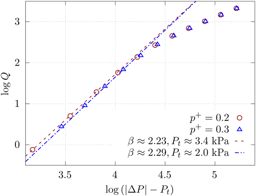
FIGURE 12. Total volumetric flow rate Q as a function of effective pressure in systems with different non-wetting grain occupation probabilities p⁺. The effective pressure is the difference between the global pressure difference |ΔP| and the threshold pressure P_t. The results of linear fit with slopes β are included in the plot, where β is the exponent in $Q\propto {\left(|\mathrm{\Delta }P|-P_t\right)}^{\beta }$. Q and |ΔP| were measured in the units of mm³/s and Pa, respectively.

6 Conclusion

We studied the effect of having porous media consisting of randomly mixed dual-wettability grains on the immiscible two-phase flow using a dynamic pore network model. The model treats the interfacial tension between the two fluids similarly to a model introduced by Irannezhad et al. [31, 32]. The model has two parameters, the saturation S_w and the probability p⁺ to have a grain of “+” type. The model, which is explained in Figure 2, contains links (pores) of three types when filled with two immiscible fluids A and B: links that are wetting with respect to fluid type A, links that are wetting with respect to fluid type B, and easy links where there are no capillary forces associated with interfaces. The parameter p⁺ controls the number of links generating capillary forces and easy links. The model has a rich phase diagram, sketched in Figure 1. There is a region 1 − p_c ≤ p⁺ ≤ p_c, where p_c is the site percolation threshold, where the easy links form connected paths across the network. Outside this region, i.e., for p⁺ ≪ 1 − p_c or p⁺ ≫ p_c, easy links do not percolate. We find two classes of constitutive equations for the volumetric flow rate Q vs. pressure drop |ΔP|. For 1 − p_c ≤ p⁺ ≤ p_c, we observed the constitutive Eq. 13—see Figure 9—whereas for p⁺ ≪ 1 − p_c or p⁺ ≫ p_c, we observed a constitutive Equation 17; see Figure 12. The crucial point that distinguishes these is whether there is a non-zero threshold pressure P_t.

When 1 − p_c ≤ p⁺ ≤ p_c, we observed the following: at the regimes with the lowest and highest |ΔP|, it seems that β = 1.00 ± 0.01 because there is no significant change in the paths fluids are flowing through, and increasing |ΔP| only increases the flow in the already active paths. At the lowest |ΔP|, the flow is mainly through connected paths with zero resistance. When p⁺ → 0.5 in this regime, there are more connected paths, which means more fluid gets transported, making Q hence M higher. At the highest |ΔP|, almost the entire network is always active. On the other hand, β > 1 in the middle regime where an increase in |ΔP| increases the flow in the active paths and, in addition, opens new conducting paths. In the middle and the highest regimes, the flow is no longer mainly through the connected paths, and the differences between the pressures across the links and the capillary barriers in the links are large. With the diminished role of the connected paths and capillary barriers at higher pressure drops, M_m and M_D do not depend strongly on p⁺. The exponent in the middle regime was found to be β = β₃ = 2.56 ± 0.05. We saw no systematic dependence of β on p⁺.

For p⁺ = 0.2, however, β = 2.23 ± 0.05 and $P_t=\left(3.4\pm 0.5\right)$ kPa, and for p⁺ = 0.3, β = 2.29 ± 0.05 and $P_t=\left(2.0\pm 0.5\right)$ kPa. Due to the necessity of determining P_t and β simultaneously at these p⁺ values, there is more uncertainty associated with the measurements of β. It is not possible to verify or falsify whether there is a fixed β = β₂, or whether it depends on p⁺ and S_w.

The existence of connecting paths is a percolation problem. They disappear when $p^{+}\to {(1-p_c)}^{+}$ or $p^{+}\to {(p_c)}^{-}$. It would, therefore, be expected that the mobility M defined in Eq. 13 would exhibit a critical behavior similar to the conductance near a critical point. By making the hypothesis that M behaves as in Eq. 14 and using finite size scaling, we determined t′ ≈ 5.7; see Figure 7. This is a huge value and raises the suspicion that the system is not critical where percolation theory dictates that it should be. Possible suspects for causing this push away from criticality are the links that do not contain interfaces. They are not easy links, but they have precisely the same effect on the dynamics of the flow as the easy links. If this is so, the transition lines would then be shifted, as shown in Figure 1.

We have only explored a small part of the phase diagram of this rich model in this first study. The phase diagram should be investigated in more detail and over a wider range of parameters. The nature of the transition lines is as of now unknown and should also be further investigated. There are percolation transitions in the model. The question as to where they are and what their properties are as the transport is not through percolation clusters remains unclear.

Data availability statement

The original contributions presented in the study are included in the article/Supplementary Material; further inquiries can be directed to the corresponding author.

Author contributions

HF performed the numerical simulations and the data analysis, and wrote the first draft of the manuscript. HF wrote the code specific for this project based on algorithms written by SS. AH and SS suggested the idea of the problem. AH worked out the relation to percolation theory. All authors contributed to the article and approved the submitted version.

Funding

This work was supported by the Research Council of Norway through its Center of Excellence funding scheme, project number 262644.

Acknowledgments

The authors would like to thank S. B. Santra and D. Jnana for discussions on the percolation problem that this system poses.

Conflict of interest

The authors declare that the research was conducted in the absence of any commercial or financial relationships that could be construed as a potential conflict of interest.

Publisher’s note

All claims expressed in this article are solely those of the authors and do not necessarily represent those of their affiliated organizations, or those of the publisher, the editors, and the reviewers. Any product that may be evaluated in this article, or claim that may be made by its manufacturer, is not guaranteed or endorsed by the publisher.

References

1 Ohm GS. Die galvanische kette, matematisch bearbeitet. Berlin: T. H. Riemann (1827).

Google Scholar

2 Darcy H. Les fontaines publiques de la ville de Dijon. Paris: Dalmont (1856).

Google Scholar

3 Whitaker S. Flow in porous media I: A theoretical derivation of Darcy's law. Transport in porous media (1986) 1:3–25. doi:10.1007/bf01036523

CrossRef Full Text | Google Scholar

4 Wyckoff R, Botset H. The flow of gas-liquid mixtures through unconsolidated sands. Physics (1936) 7:325–45. doi:10.1063/1.1745402

CrossRef Full Text | Google Scholar

5 Barenblatt G, Patzek T, Silin D. The mathematical model of non-equilibrium effects in water-oil displacement. In: Spe/doe improved oil recovery symposium. Richardson, TX: OnePetro (2002).

Google Scholar

6 Tallakstad KT, Knudsen HA, Ramstad T, Løvoll G, Måløy KJ, Toussaint R, et al. Steady-state two-phase flow in porous media: Statistics and transport properties. Phys Rev Lett (2009) 102:074502. doi:10.1103/physrevlett.102.074502

PubMed Abstract | CrossRef Full Text | Google Scholar

7 Tallakstad KT, Løvoll G, Knudsen HA, Ramstad T, Flekkøy EG, Måløy KJ. Steady-state, simultaneous two-phase flow in porous media: An experimental study. Phys Rev E (2009) 80:036308. doi:10.1103/physreve.80.036308

CrossRef Full Text | Google Scholar

8 Rassi EM, Codd SL, Seymour JD. Nuclear magnetic resonance characterization of the stationary dynamics of partially saturated media during steady-state infiltration flow. New J Phys (2011) 13:015007. doi:10.1088/1367-2630/13/1/015007

CrossRef Full Text | Google Scholar

9 Aursjø O, Erpelding M, Tallakstad KT, Flekkøy EG, Hansen A, Måløy KJ. Film flow dominated simultaneous flow of two viscous incompressible fluids through a porous medium. Front Phys (2014) 2:63. doi:10.3389/fphy.2014.00063

CrossRef Full Text | Google Scholar

10 Sinha S, Bender AT, Danczyk M, Keepseagle K, Prather CA, Bray JM, et al. Effective rheology of two-phase flow in three-dimensional porous media: Experiment and simulation. Transport in porous media (2017) 119:77–94. doi:10.1007/s11242-017-0874-4

PubMed Abstract | CrossRef Full Text | Google Scholar

11 Gao Y, Lin Q, Bijeljic B, Blunt MJ. Pore-scale dynamics and the multiphase Darcy law. Phys Rev Fluids (2020) 5(1):013801. doi:10.1103/physrevfluids.5.013801

CrossRef Full Text | Google Scholar

12 Zhang Y, Bijeljic B, Gao Y, Lin Q, Blunt MJ. Quantification of nonlinear multiphase flow in porous media. Geophys Res Lett (2021) 48(5). doi:10.1029/2020gl090477

CrossRef Full Text | Google Scholar

13 Zhang Y, Bijeljic B, Blunt MJ. Nonlinear multiphase flow in hydrophobic porous media. J Fluid Mech (2022) 934:R3. doi:10.1017/jfm.2021.1148

CrossRef Full Text | Google Scholar

14 Grøva M, Hansen A. Two-phase flow in porous media: Power-law scaling of effective permeability. J Phys Conf Ser (2011) 319:012009. doi:10.1088/1742-6596/319/1/012009

CrossRef Full Text | Google Scholar

15 Sinha S, Hansen A. Effective rheology of immiscible two-phase flow in porous media. Europhysics Lett (2012) 99:44004. doi:10.1209/0295-5075/99/44004

CrossRef Full Text | Google Scholar

16 Sinha S, Hansen A, Bedeaux D, Kjelstrup S. Effective rheology of bubbles moving in a capillary tube. Phys Rev E (2013) 87(2):025001. doi:10.1103/physreve.87.025001

CrossRef Full Text | Google Scholar

17 Xu X, Wang X. Non-Darcy behavior of two-phase channel flow. Phys Rev E (2014) 90(2):023010. doi:10.1103/physreve.90.023010

CrossRef Full Text | Google Scholar

18 Yiotis A, Dollari A, Kainourgiakis M, Salin D, Talon L. Nonlinear Darcy flow dynamics during ganglia stranding and mobilization in heterogeneous porous domains. Phys Rev Fluids (2019) 4(11):114302. doi:10.1103/physrevfluids.4.114302

CrossRef Full Text | Google Scholar

19 Roy S, Hansen A, Sinha S. Effective rheology of two-phase flow in a capillary fiber bundle model. Front Phys (2019) 7:92. doi:10.3389/fphy.2019.00092

CrossRef Full Text | Google Scholar

20 Roy S, Sinha S, Hansen A. Immiscible two-phase flow in porous media: Effective rheology in the continuum limit (2019). Available at: https://arxiv.org/abs/1912.05248 (Accessed December 11, 2019).

Google Scholar

21 Fyhn H, Sinha S, Roy S, Hansen A. Rheology of immiscible two-phase flow in mixed wet porous media: Dynamic pore network model and capillary fiber bundle model results. Transport in Porous Media (2021) 139:491–512. doi:10.1007/s11242-021-01674-3

CrossRef Full Text | Google Scholar

22 Sales J, Seybold HJ, Oliveira CL, Andrade JS. Bubble dynamics in stationary two-phase flow through disordered porous media. Front Phys (2022) 170. doi:10.3389/fphy.2022.860190

CrossRef Full Text | Google Scholar

23 Feder J, Flekkøy EG, Hansen A. Physics of flow in porous media. Cambridge: Cambridge University Press (2022).

Google Scholar

24 Lanza F, Rosso A, Talon L, Hansen A. Non-Newtonian rheology in a capillary tube with varying radius. Transport in Porous Media (2022) 145(1):245–69. doi:10.1007/s11242-022-01848-7

CrossRef Full Text | Google Scholar

25 Cheon HL, Fyhn H, Hansen A, Wilhelmsen Ø, Sinha S. Steady-state two-phase flow of compressible and incompressible fluids in a capillary tube of varying radius. Transport in Porous Media (2023) 147:15–33. doi:10.1007/s11242-022-01893-2

CrossRef Full Text | Google Scholar

26 Wilkinson D. Percolation effects in immiscible displacement. Phys Rev A (1986) 34:1380–91. doi:10.1103/physreva.34.1380

CrossRef Full Text | Google Scholar

27 Stauffer D, Aharony A. Introduction to percolation theory. Abingdon, UK: Taylor & Francis (2018).

Google Scholar

28 Roux S, Herrmann H. Disorder-induced nonlinear conductivity. Europhys Lett (1987) 4(11):1227–31. doi:10.1209/0295-5075/4/11/003

CrossRef Full Text | Google Scholar

29 Scheidegger AE. Theoretical models of porous matter. Prod Monthly (1953) 17:17.

Google Scholar

30 Scheidegger AE. The physics of flow through porous media. 3rd. Toronto: University of Toronto press (2020).

Google Scholar

31 Irannezhad A, Primkulov BK, Juanes R, Zhao B. Fluid-fluid displacement in mixed-wet porous media. Phys Rev Fluids (2023) 8:L012301. doi:10.1103/PhysRevFluids.8.L012301

CrossRef Full Text | Google Scholar

32 Irannezhad A, Primkulov BK, Juanes R, Zhao B. Characteristics of fluid-fluid displacement in model mixed-wet porous media: patterns, pressures, and scalings (2006). Available at: https://arxiv.org/abs/2302.03072 (Accessed February 6, 2023).

Google Scholar

33 Knudsen HA, Hansen A. Two-phase flow in porous media: Dynamical phase transition. Eur Phys J B-Condensed Matter Complex Syst (2006) 49:109–18. doi:10.1140/epjb/e2006-00019-y

CrossRef Full Text | Google Scholar

34 Grossman T, Aharony A. Structure and perimeters of percolation clusters. J Phys A: Math Gen (1986) 19:L745–51. doi:10.1088/0305-4470/19/12/009

CrossRef Full Text | Google Scholar

35 Redner S. Fractal and multifractal scaling of electrical conduction in random resistor networks (2007). Available at: https://arxiv.org/abs/0710.1105 (Accessed October 4, 2007).

Google Scholar

36 Sinha S, Gjennestad MA, Vassvik M, Hansen A. Fluid meniscus algorithms for dynamic pore-network modeling of immiscible two-phase flow in porous media. Front Phys (2021) 8:567. doi:10.3389/fphy.2020.548497

CrossRef Full Text | Google Scholar

37 Aker E, Måløy KJ, Hansen A, Batrouni GG. A two-dimensional network simulator for two-phase flow in porous media. Transport in porous media (1998) 32(2):163–86. doi:10.1023/a:1006510106194

CrossRef Full Text | Google Scholar

38 Knudsen HA, Aker E, Hansen A. Bulk flow regimes and fractional flow in 2D porous media by numerical simulations. Transport in Porous Media (2002) 47:99–121. doi:10.1023/a:1015039503551

CrossRef Full Text | Google Scholar

39 Tørå G, Øren P-E, Hansen A. A dynamic network model for two-phase flow in porous media. Transport in Porous Media (2012) 92(1):145–64. doi:10.1007/s11242-011-9895-6

CrossRef Full Text | Google Scholar

40 Gjennestad MA, Vassvik M, Kjelstrup S, Hansen A. Stable and efficient time integration of a dynamic pore network model for two-phase flow in porous media. Front Phys (2018) 6:56. doi:10.3389/fphy.2018.00056

CrossRef Full Text | Google Scholar

41 Sinha S, Grøva M, Ødegården TB, Skjetne E, Hansen A. Local wettability reversal during steady-state two-phase flow in porous media. Phys Rev E (2011) 84(3):037303. doi:10.1103/physreve.84.037303

CrossRef Full Text | Google Scholar

42 Flovik V, Sinha S, Hansen A. Dynamic wettability alteration in immiscible two-phase flow in porous media: Effect on transport properties and critical slowing down. Front Phys (2015) 3:86. doi:10.3389/fphy.2015.00086

CrossRef Full Text | Google Scholar

43 Blunt MJ. Multiphase flow in permeable media: A pore-scale perspective. Cambridge: Cambridge University Press (2017).

Google Scholar

44 Straley JP. Critical exponents for the conductivity of random resistor lattices. Phys Rev B (1977) 15(12):5733–7. doi:10.1103/physrevb.15.5733

CrossRef Full Text | Google Scholar

45 Xun Z, Hao D, Ziff RM. Site percolation on square and simple cubic lattices with extended neighborhoods and their continuum limit. Phys Rev E (2021) 103:022126. doi:10.1103/physreve.103.022126

PubMed Abstract | CrossRef Full Text | Google Scholar

46 Cen W, Liu D, Mao B. Molecular trajectory algorithm for random walks on percolation systems at criticality in two and three dimensions. Physica A: Stat Mech its Appl (2012) 391(4):925–9. doi:10.1016/j.physa.2011.01.003

CrossRef Full Text | Google Scholar

47 Den Nijs M. A relation between the temperature exponents of the eight-vertex and q-state Potts model. J Phys A: Math Gen (1979) 12(10):1857–68. doi:10.1088/0305-4470/12/10/030

CrossRef Full Text | Google Scholar

48 Erpelding M, Sinha S, Tallakstad KT, Hansen A, Flekkøy EG, Måløy KJ. History independence of steady state in simultaneous two-phase flow through two-dimensional porous media. Phys Rev E (2013) 88(5):053004. doi:10.1103/physreve.88.053004

CrossRef Full Text | Google Scholar