The resonance between the electromagnetic field and electrons in the helicon plasma source of a magnetoplasma rocket engine

1 Introduction

The magnetoplasma rocket engine (MPRE) is a high-power electromagnetic thruster with the technical advantages of high specific impulse, high thrust, and high efficiency, which can be deployed in the exploration for deep space and other missions. The engine originates from the magnetic confinement fusion and comprises three, linked but distinct, magnetic stages serving different but complementary processes that are shown in Figure 1 [1]. In the first stage, the helicon plasma source produces high-density, low-temperature plasma; in the second stage, “the rf heater” receives this plasma and preferentially heats the ion population to hundreds of eV by ion cyclotron resonance heating (ICRH); and in the third stage, the magnetic nozzle is the diverging section of the magnetic field, where the heated plasma naturally accelerates and leaves the device to produce a rocket thrust [1, 2].It should be noted that the MPRE can work with multiple kinds of propellant species (Ar, Kr, and Xe), while Ar is used merely as an example in the figure. According to the working principles of the MPRE, the helicon plasma source provides sufficient plasma for the engine which lays the foundation for the engine to generate thrust.

FIGURE 1

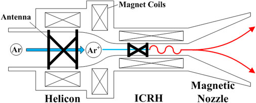
FIGURE 1. Schematic of the MPRE.

Compared with other kinds of rf sources, the helicon plasma source depends on the excitation of bounded whistle waves to generate high-density plasma at low pressures and rf power [3]. Due to the efficient power deposition, the plasma density in the helicon plasma source is hundreds of times higher than that in other plasma sources at a given power. As a result, the helicon plasma source has been widely used in space propulsion [4–6].

Since high-density plasma in the helicon plasma source was first reported by Boswell in 1970 [7], the helicon plasma source has been the subject of intensive research. The research mainly focuses on the power deposition mechanism and the wave mode recognition. At first, the mechanism of Landau damping proposed by F F Chen was thought to be the way by which power is deposited [8]. However, subsequent experiments showed that the Landau-accelerated electrons are too sparse to account for the high ionization efficiency, and the mechanism of Landau damping was denied by F F Chen and D D Blackwell [9, 10]. In the dispersion relation of the helicon plasma [11], there are two branches of waves, one is the helicon wave and the other is known as the “Trivelpiece–Gould wave” (TG wave) [12]. It is more appropriate to account for the deposition of power by the strong damping of the TG wave [13–16].To date, the mechanism of the helicon plasma source is unclear and needs further research. In addition to the power deposition mechanism, there is a unique phenomenon in the helicon plasma source that the plasma density jumps at a certain power, together with the conversion of the operation mode [17, 18]. F F Chen thought it is the result of the impedance non-monotonic variation [19]. S H Kim proposed the concept of mode conversion surface (MCS) for mode conversion [20], while Mingyang WU thought it is the formation of the standing helicon wave (SHW) that triggers mode conversion [21].

The helicon plasma source must produce a plasma stream with a high degree of ionization for the application of ICRH power to enable an effective propulsion device [1, 2]. The research for the helicon plasma source will be significant to the development of the MPRE. However, it is extremely difficult to make direct measurements of the plasma or the electromagnetic field in the discharge chamber due to the limitation of the engine structure [22]. Therefore, numerical simulation has become an economical and effective alternative method to study the helicon plasma source. In the existing numerical models, the simulation of the helicon plasma source is usually performed with a uniform magnetic field, while the magnetic field in the MPRE is much more complicated. For such reasons, a numerical model that contains a practical magnetic field needs to be developed.

In this paper, a multi-fluid, two-dimensional, axisymmetric model coupled with the electromagnetic field was developed to simulate the helicon plasma source in the MPRE. The simulation was performed using different magnetic fields to analyze the mechanism of mode conversion and power deposition. This paper is organized as follows. Section 2 is the governing equations of the model; the simulation model is set up in Section 3; Section 4 is the discussion of the results; and in Section 5, the results are concluded.

2 Governing equations

The transportation of electrons, ions, atoms, and the interactions with the electromagnetic field, as well as the electrostatic field, is included in the simulation model. In this section, the equations of the electromagnetic field, charged particles, neutral atoms, and electrostatic field in the cylindrical coordinate system (r, θ, and z) are introduced.

2.1 Electromagnetic field

Maxwell equations and current density (Eq. 3) are solved to obtain the electromagnetic field.

$\nabla \times {\mathit{H}}_{rf}={\epsilon }_0\frac{\partial {\mathit{E}}_{rf}}{\partial t}+{\mathit{J}}_{total},(1)$

$\nabla \times {\mathit{E}}_{rf}=-\frac{\partial {\mathit{H}}_{rf}}{\partial t},(2)$

$\frac{\partial {\mathit{J}}_j}{\partial t}=\frac{n_j{q}_j^2}{m_j}{\mathit{E}}_{rf}+\frac{q_j}{m_j}{\mathit{J}}_j\times \mathit{B}-{\nu }_{jn}{\mathit{J}}_j,(3)$

${\mathit{J}}_{total}={\mathit{J}}_i+{\mathit{J}}_e+{\mathit{J}}_{input},(4)$

where the subscript rf refers to the fields that are excited by the rf input and subscript j refers to different charged particles (ions and electrons). H and E are the magnetic field intensity and the electric field intensity, respectively. ε₀ is the vacuum permittivity, and μ₀ is the vacuum permeability. q_j, n_j, m_j, and J_j are the charge, density, mass, and current density of charged particles, respectively. ν_jn is the collision frequency between charged particles and atoms. B is the static magnetic field. J_input is the input current density that excites the electromagnetic wave. J_total is the total current density of the plasma current density and the input current density. In the cylindrical coordinate system, the solutions of Maxwell equations are divided into the transverse-magnetic (TM) mode and the transverse-electric (TE) mode whose equations are shown in as follows:

$\left\{\begin{array}{c}{\mu }_0\frac{\partial H_r}{\partial t}=-\frac{1}{r}\frac{\partial E_z}{\partial \theta }+\frac{\partial E_{\theta }}{\partial z}\\ {\epsilon }_0\frac{\partial E_{\theta }}{\partial t}=\frac{\partial H_r}{\partial z}-\frac{\partial H_z}{\partial r}-J_{\theta }\\ {\mu }_0\frac{\partial H_Z}{\partial t}=-\frac{1}{r}{E}_{\theta }-\frac{\partial E_{\theta }}{\partial r}+\frac{1}{r}\frac{\partial E_r}{\partial \theta },\end{array}\right.(5)$

$\left\{\begin{array}{c}{\epsilon }_0\frac{\partial E_r}{\partial t}=\frac{1}{r}\frac{\partial H_z}{\partial \theta }-\frac{\partial H_{\theta }}{\partial z}-J_r\\ {\mu }_0\frac{\partial H_{\theta }}{\partial t}=-\frac{\partial E_r}{\partial z}+\frac{\partial E_z}{\partial r}\\ {\epsilon }_0\frac{\partial E_Z}{\partial t}=\frac{1}{r}{H}_{\theta }+\frac{\partial H_{\theta }}{\partial r}-\frac{1}{r}\frac{\partial H_r}{\partial \theta }-J_z,\end{array}\right.(6)$

where the subscript rf is omitted for simplicity. After the current density field and the electric field are obtained, the deposit power density of different particles is the dot product of these two fields.

$P_j={\mathit{J}}_j\bullet {\mathit{E}}_{rf}.(7)$

2.2 Charged particles

The drift–diffusion equations are used for the transportation of charged particles [21, 23]. Equation 8 is the number density equation, and Eq. 9 is the energy equation.

$\frac{\partial n_j}{\partial t}+\nabla \bullet {\mathit{\Gamma }}_j=K_{ion}{n}_e{n}_n,(8)$

$\begin{array}{c}\frac{\partial }{\partial t}\left(\frac{3}{2}{n}_j{k}_B{T}_j\right)+\nabla \bullet {\mathit{Q}}_j=P_j-{\delta }_{je}\left({\epsilon }_{ion}{K}_{ion}+{\epsilon }_{exc}{K}_{exc}\right)n_e{n}_n+q_j{\mathit{\Gamma }}_j\bullet {\mathit{E}}_s\\ {\delta }_{je}=\left\{\begin{array}{c}1j=e\\ 0j\ne e,\end{array}\right.\end{array}(9)$

where Γ_j is the flux density and n_n is the density of neutral atoms. K_ion and K_exc are the ionization rate and excitation rate, respectively. T_j and Q_j are the particle temperature and the energy flux density, respectively. ε_ion and ε_exc are the threshold energy of ionization and excitation. E_s is the electrostatic field. The Kronecker symbol δ_je indicates the second term on the right hand side of Eq. 9, which only appears in the energy equation of the electron. The particle flux density and energy flux density are given in the following equations:

${\mathit{\Gamma }}_j={\mu }_j\left(n_j{\mathit{E}}_s+{\mathit{\Gamma }}_j\times \mathit{B}\right)-D_j\nabla n_j,(10)$

${\mathit{Q}}_j=-\frac{3}{2}{k}_B{D}_j{n}_j\nabla T_j+\frac{5}{2}{k}_B{T}_j{\mathit{\Gamma }}_j,(11)$

where μ_j is the particle mobility and D_j is the diffusion coefficient. In this model, the working medium is Ar and the ionization and excitation collisions are under consideration. The reaction rate is calculated by the electron thermal velocity and collision sections. The collision sections coming from the database of Morgan are weighted by Maxwell distribution to obtain the reaction rates. In the simulation, K_ion and K_exc are set according to the local electron temperature.

2.3 Neutral atoms

Since the atoms will not be heated by the rf field, only the continuity (Eq. 12) and the momentum (Eq. 13) are solved to obtain the number density of atoms in the computation domain.

$\frac{\partial n_n}{\partial t}+\nabla \bullet \left(n_n{\mathit{v}}_n\right)=-K_{ion}{n}_e{n}_n,(12)$

$\frac{\partial \left(n_n{\mathit{v}}_n\right)}{\partial t}+\nabla \bullet \left(n_n{\mathit{v}}_n{\mathit{v}}_n\right)=-\frac{k_B{T}_j}{m_n}\nabla n_n.(13)$

Here, m_n, v_n, and T_n are the atom mass, velocity, and temperature, respectively.

2.4 Electrostatic field

In order to make Eqs 8, 9 closer, the electrostatic filed is also needed to obtain the particle flux density and the energy flux density. The electrostatic field is obtained by using the solution of the semi-implicit Poisson equation [24].

${\nabla }^{2}V\left(t+∆t\right)=-\frac{e}{{\epsilon }_0}\left[\left(n_i-n_e\right)+∆t\left(\nabla \bullet {\mathit{\Gamma }}_e-\nabla \bullet {\mathit{\Gamma }}_i\right)\right],(14)$

where V is the electrostatic potential and Δt is the time step. The divergence of the particle flux is added in the right-hand side to predict the potential of the next step, which is effective to increase the time step [21]. The electrostatic field is the negative gradient of the electrostatic potential V.

3 Simulation model setup

The numerical algorithm, initialization, and reliability of the model are introduced in this section.

3.1 Numerical algorithm

The alternating-direction implicit finite-difference time-domain (ADI-FDTD) method is adopted to solve Eqs 1–3 [25].The updation of the electromagnetic field in one time step is divided into two separate steps, and the implicit scheme is first observed in the z-direction and then in the r-direction. In ADI-FDTD, the time step can break through the limitation of the Courant–Friedrich–Levy (CFL) condition to accelerate time integration.

The density and temperature of the charged particles are discretized with the staggered grid and are integrated by the implicit scheme. In the staggered grid, n_j and T_j are placed at the grid points, while T_j and Q_j are placed at the midpoints of the grids, which can be seen in [22]. In the implicit scheme, the time derivatives observed in Eqs 8, 9 are calculated with the variables of the next time step and the equations are solved with an iterative method.

The equations of neutral atoms are solved using the flux-corrected transport (FCT) algorithm [26], which has been proven to be an accurate and user-friendly algorithm for the solution of non-linear, time-dependent continuity equations in fluid and plasma dynamics. The split-step approach is adopted in time integration in which the integration of the z- and r-direction is alternated. Detailed information of the FCT algorithm and the test codes can be seen in [26].

Poisson’s equation (Eq. 14) is solved using the five-point difference scheme.

3.2 Initialization

Figure 2 is a schematic of the geometric model. The computation domain is an axisymmetrical cylinder with a radius of 0.1 m and length 0.5 m. The plasma is in a cylindrical chamber with a radius of 0.06 m. The input current of the helicon plasma source is placed at (z_c1 and r_c1), and that of ICRH is placed at (z_c2 and r_c2). In the simulation, z_c1 and r_c1 are set to be 0.15 m and 0.07 m, respectively. The input current density J_input is calculated by Eq. 15, where Δz and Δr are the grid size of the z- and r-direction, respectively. I_input and f_input are the input current and the input frequency that are set to be 60A and 13.56 MHz, respectively. ICRH is beyond the scope of this paper, and it will be discussed in the future.

$J_{input}=\frac{I_{input}}{∆z∆r}\sin \left(2\pi f_{input}t\right)(15)$

FIGURE 2

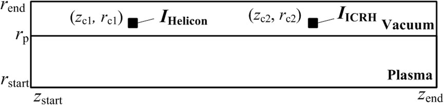
FIGURE 2. Schematic of the geometric model.

In the solution of the electromagnetic field, the implicit MUR condition is adopted to prevent reflection at the boundary. At the plasma boundary, n_j = 0 and V = 0 [21]. All variables adopted the symmetric boundary at the axis.

Figure 3 shows the profile of the background magnetic field. There exist uniform sections upstream of the field, and the magnetic induction intensity is 0.005T, 0.01T, 0.02T, and 0.05T. At the initial moment, n_j = 1.0 × 10¹⁶m^-3, T_e = 2eV, and T_i = T_n = 300 K. Atom density is set according to the pressure, which is set to be 0.42 Pa. The program was coded with Fortran, and the calculation data are dumped every rf cycle until all variables become steady.

FIGURE 3

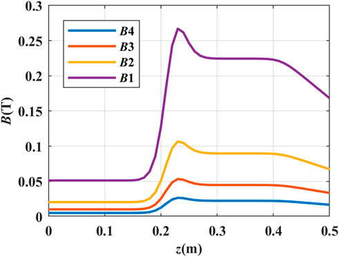
FIGURE 3. Profile of the background magnetic field along the axis.

3.3 Reliability and validation of the model

The ICP source was simulated, and the results were compared with other models to verify the reliability of the model in this paper. In the simulation, z_end, r_end, r_p, z_c1, and r_c1 were set to be 0.4 m, 0.125 m, 0.075 m, 0.3 m, and 0.09 m, respectively. The pressure was 2.6 Pa. The electron density distributions of different models are shown in Figure 4. Figure 4A shows the result of Peking University Helicon Discharge (PHD) software, while Figure 4B shows the result of COMSOL [21, 27]software. The figures show that the plasma distributions are the same in three models, which indicates the plasma transportation in different models is consistent. The input power of PHD and COMSOL is 500 W, while the input parameter of this paper is the current that is set to be 50 A. Due to the different input methods, the absolute value of electron density in this paper is different compared with other models. Figure 5 shows the electron density along the radial direction at z = 0.3m, which is normalized by the density at the axis. The three models have the largest difference at r = 0.065, and the difference with PHD and COMSOL is 7.14% and 13.39%, respectively.

FIGURE 4

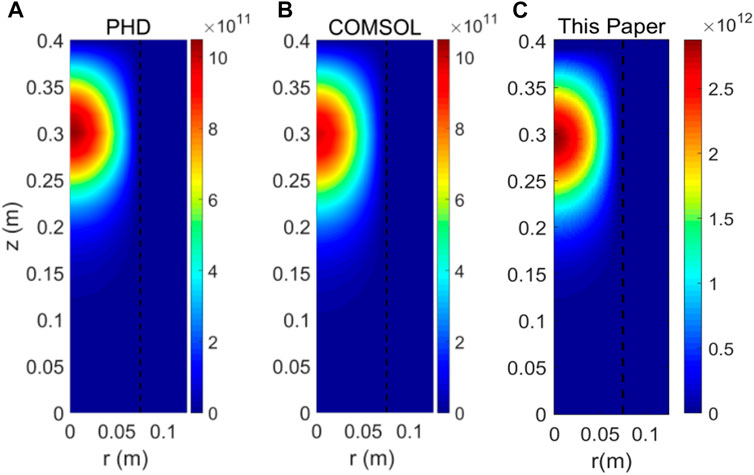
FIGURE 4. Distribution of electron density in different models: (A) PHD, (B) COMSOL, and (C) the model in this paper [21, 27].

FIGURE 5

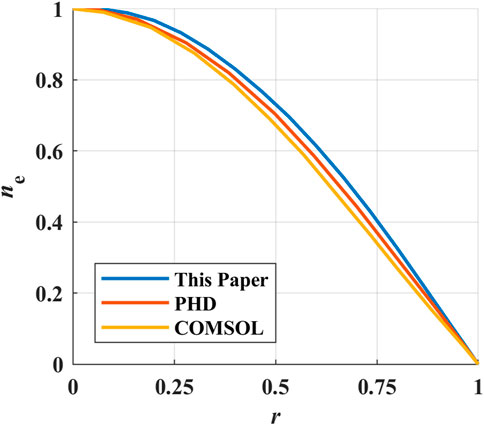
FIGURE 5. Normalized electron density along the radial direction at z = 0.3 m.

The aforementioned comparison shows that the results of the model in this paper are very similar to those of other models, which verifies the reliability of the model.

4 Results

4.1 Mode conversion in the helicon plasma source

It is shown in [28] that there exist several modes in the helicon plasma source, namely, the capacitive mode (E mode), inductive mode (H mode), and wave mode (W mode) of different orders, W₁, W₂, W₃. . . . The mode conversion is always accompanied by the plasma density jump. In the model of this paper, no E mode exists since the wall voltage is 0 V. Therefore, only the H mode and the different W modes will appear.

Figure 6 shows the maximum electron density and the maximum electron temperature during the simulation with the magnetic field B1 (helicon plasma source) and without the magnetic field (ICP source). The dotted line represents the data obtained after all variables become steady. First, it can be seen that the electron density gradually increases under the action of the rf input. The electron density at the steady state of the two sources is 4.37 × 10¹⁹ m^-3 and 2.37 × 10¹⁷ m^-3. With the same input current, the plasma density of the helicon plasma source is 184 times higher than that of the ICP source. The electron temperature of the helicon plasma source is 2.63 eV, which is consistent with typical values in cold plasma. Second, Figure 6 shows the evolution of electron density and temperature in two kinds of plasma sources is of great difference. The growth rate of the electron density in the ICP source increases first and then decreases, and the curve is much smoother. However, there are several peaks in the curve of electron temperature in the helicon plasma source. Due to the sudden increase of electron temperature, the ionization term in Eq. 8 gets larger and the electron density increases dramatically in a few rf cycles. As a result, several inflection points in the electron density curve are observed, which make the density curve look like a stair. According to the results in [28], it can be inferred from Figure 6 that the coupling mode between plasma and the electromagnetic field changes with time in the helicon plasma source.

FIGURE 6

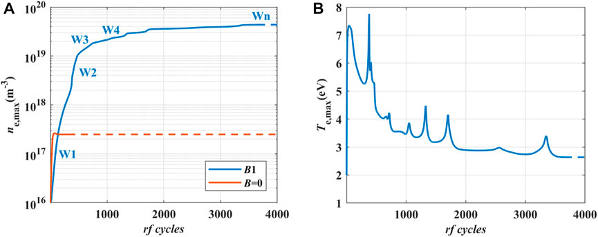
FIGURE 6. (A) Maximum electron density and (B) maximum electron temperature during discharge.

In the rf plasma source, the plasma accomplishes the discharge with the deposit power from the external electromagnetic field. The difference between plasma parameters should come from the difference of power deposition. The deposit power density of electrons at different moments of the ICP source is shown in Figure 7. The rfc in the figure refers to the rf cycles. The deposit power density reaches the maximum value at the point which is closer to the input position, and the configuration does not change with time. When there is no magnetic field, the solution of Maxwell equations only contains the TM mode in Eq. 5. As a result, only E_θ is not 0 among the components of electric fields and all the deposit power comes from the θ-direction. Therefore, the ICP source is always in the H mode, and the configuration of the deposit power density will not change with plasma parameters.

FIGURE 7

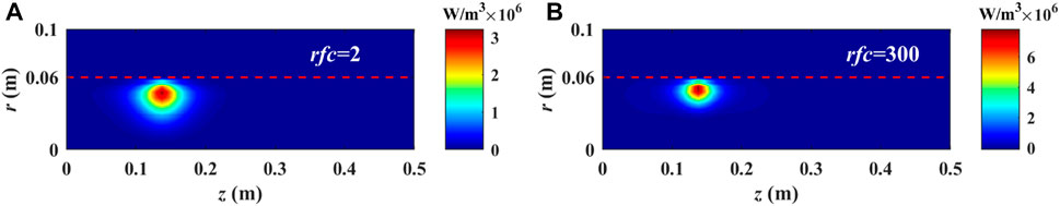
FIGURE 7. Deposit power density of electrons at different moments of the ICP source: (A) rfc = 2 and (B) rfc = 300.

Figure 8 shows the deposit power density at different moments of the helicon plasma source. First, it can be seen that the deposit power density is mainly located upstream of the computation domain due to the configuration of the magnetic field. In addition, the distribution of deposit power density continuously changes with time. In the beginning, the deposit power is concentrated in a thin layer near the edge of the plasma and the power density in this layer gradually increases, as shown in Figures 8A, B. Then, the power density inside the plasma begins to increase. Figure 8C shows that when the plasma density is about 2 × 10¹⁸ m⁻³, the deposit power near the axis plays a major role in the power deposition. Subsequently, the configuration of deposit power density continues to change until the 3670th rf cycle, and the deposit power density finally becomes steady, as shown in Figure 8F. It is found in the simulation that every time the configuration of deposit power density changes, the electron temperature peak appears and leads to the dramatic increase of plasma density. The changes of deposit power density also indicate that the operation mode of the helicon plasma source does change as plasma density grows, and it can be regarded as a symbol of mode conversion.

FIGURE 8

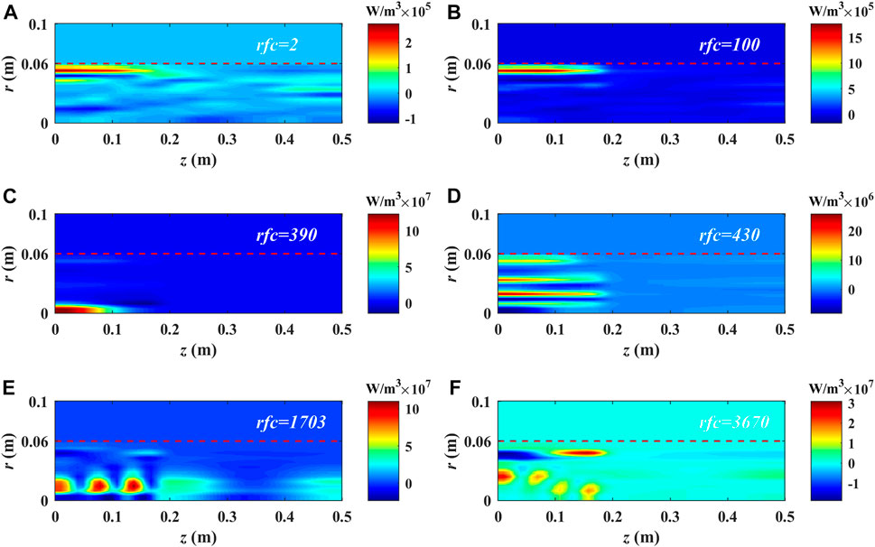
FIGURE 8. Deposit power density of electrons at different moments of the helicon plasma source: (A) rfc = 2, (B) rfc = 100, (C) rfc = 390, (D) rfc = 430, (E) rfc = 1703, and (F) rfc = 3670.

4.2 Resonance between the electric field and electrons

The deposit power density is the dot product of the electric field and electron current density. To show the characteristics of different modes, the components of the electric field and electron current density in three directions at different moments are shown in Figure 9. The results were interpolated by the spline interpolation, and the circles represent the raw data. The results at the second rf cycle that is not shown for the helicon plasma source are in the same mode when rfc = 2 and rfc = 100. The plasma becomes anisotropic when the magnetic field is not 0. For such reasons, the TM mode and the TE mode both exist and the electromagnetic field becomes much more complicated. At the 100th rf cycle, E_θ is monotonic in the radial direction. Additionally, other components are increases near the plasma edge and decrease inwards, which coincides with the characteristics of the TG wave. At this moment, the helicon plasma source is in the mode corresponding to W1, as shown in Figure 6A. When rfc = 390, the wavelength of E_θ becomes evidently shorter and the amplitudes of other components inside the plasma become larger, indicating the electromagnetic wave has penetrated into the plasma. The characteristics of the wave are similar to those of the helicon wave, and the helicon plasma source has converted from W1 to W2. Then, the wavelength of E_θ becomes shorter and shorter, as can been seen in Figures 9H, K, N. Meanwhile, the order of the wave mode becomes larger, and the mode at the steady state is represented by Wn. The aforementioned analysis suggests that it is the change of the electromagnetic field that triggers the mode conversion of the helicon plasma source. In addition, the change of E_θ is also a symbol of mode conversion.

FIGURE 9

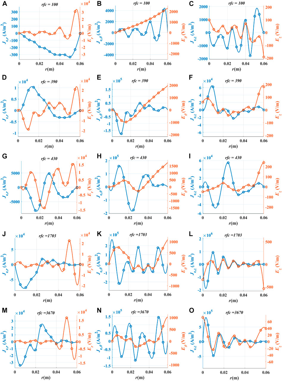
FIGURE 9. Components of the electric field and electron current density of different moments at z = 0.15 m: (A) E_r, J_e,r, rfc = 100; (B) E_θ, J_e,θ, rfc = 100; (C) E_z, J_e,z, rfc = 100; (D) E_r, J_e,r, rfc = 390; (E) E_θ, J_e,θ, rfc = 390; (F) E_z, J_e,z, rfc = 390; (G) E_r, J_e,r, rfc = 430; (H)E_θ, J_e,θ, rfc = 430; (I) E_z, J_e,z, rfc = 430; (J) E_r, J_e,r, rfc = 1703; (K) E_θ, J_e,θ, rfc = 1703; (L) E_z, J_e,z, rfc = 1703; (M) E_r, J_e,r, rfc = 3670; (N) E_θ, J_e,θ, rfc = 3670; and (O) E_z, J_e,z, rfc = 3670.

In addition to mode conversion, there is also an important phenomenon observed in Figure 9. In the high-order wave mode, E_z and J_e,z overlap with each other, as shown in Figure 9L and Figure 9O. The overlap suggests that the electric field resonates with electrons in the high-order wave mode. Figure 10 shows the deposit power density of different moments at z = 0.15 m. Figures 10A–E show that when the helicon plasma source has not converted into the high-order wave mode, P_z is so small that it almost has no contribution to the total deposit power density. All the deposit power comes from P_θ and P_r, which is in the direction perpendicular to the magnetic field. Once the resonance occurs, P_z inside the plasma increases significantly and takes the dominant part of the total deposit power density. The electron motion in the z-direction is not confined by the magnetic field so that the resonance with the electric field can excite a large current density. As a result, the deposit power of the plasma increases dramatically in the high-order wave mode. Owing to the jump of the deposit power, the plasma density in the helicon plasma source is two orders of magnitude higher than that in the ICP source.

FIGURE 10

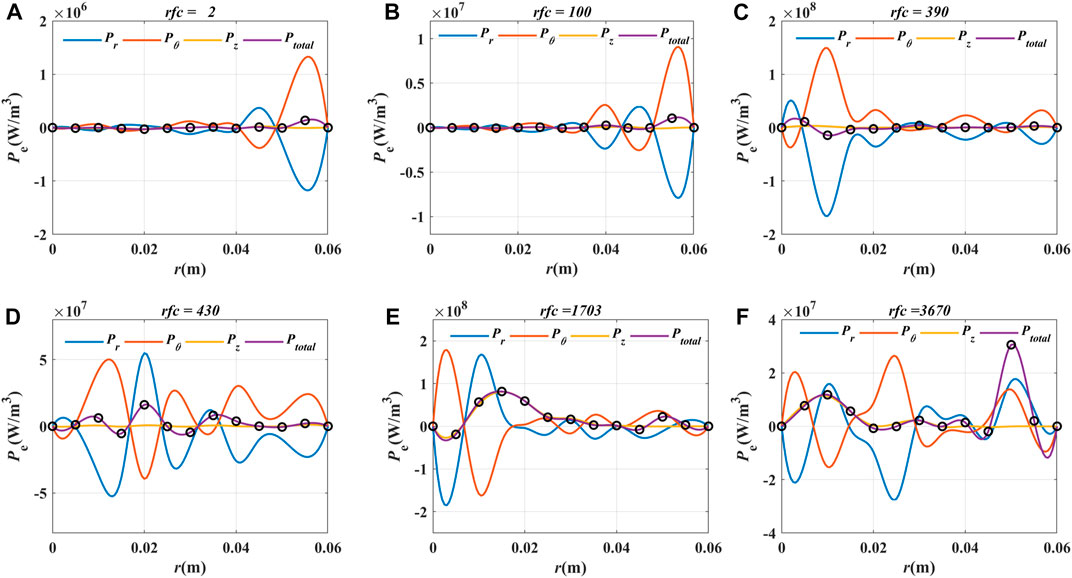
FIGURE 10. Deposit power density of electrons of different moments at z = 0.15 m: (A) rfc = 2, (B) rfc = 100, (C) rfc = 390, (D) rfc = 430, (E) rfc = 1703, and (F) rfc = 3670.

For further analysis of the power deposition mechanism in the high-order wave mode, E_θ and -J_e,r, E_r and J_e,θ, and E_z and J_e,z are drawn in the same axis, as shown in Figure 11. The results show that all the components of electron current density resonate with the electric field. However, except for J_e,z, the electron current does not resonate with the electric field in the same direction due to the anisotropy of magnetized plasma. It is E_θ and J_e,r and E_r and J_e,θ that couple with each other in the resonant state, as seen in Figures 11A, B, D, E. Consequently, P_θ and P_r cancel out because E_θ and -J_e,r and E_r and J_e,θ have the same phase position in space. Therefore, the deposit power in the high-order wave mode almost comes from the interaction in the z-direction, according to Eq. 7.

FIGURE 11

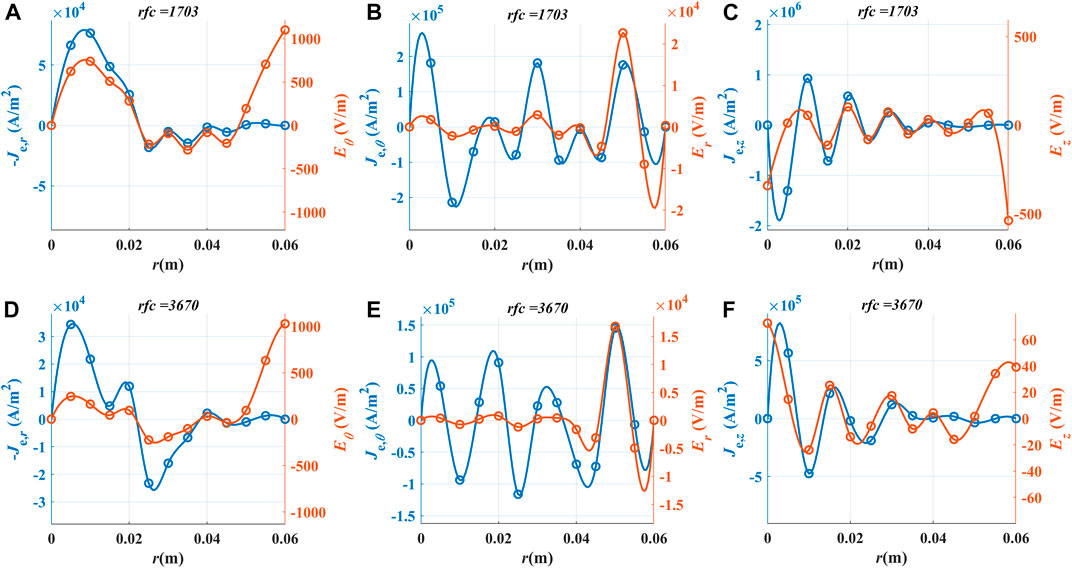
FIGURE 11. Components of the electric field and electron current density of different moments at z = 0.15 m: (A) E_θ, -J_e,r, rfc = 1703; (B) E_r, J_e,θ, rfc = 1703; (C) E_z, J_e,z, rfc = 1703; (D) E_θ, -J_e,r, rfc = 3670; (E) E_r, J_e,θ, rfc = 3670; and (F) E_z, J_e,z, rfc = 3670.

4.3 Discharge with different magnetic fields

In the helicon plasma source, the mode conversion occurs accompanied by the plasma density jump at a certain rf power or magnetic field intensity [29]. The step increment of the plasma density when varying the magnetic field intensity should come from two reasons: (1)the confinement of the magnetic field on the plasma gets stronger as the magnetic field intensity increases; (2)the configuration of the deposition power density changes when the magnetic field intensity increases, which leads to the mode conversion of the helicon plasma source. It can be seen from the governing equations of the charged particles and the electromagnetic field that the influences of the background magnetic field on the plasma transportation and the solution of the electromagnetic field are within the model presented in this paper. Therefore, the model is capable of simulating the helicon plasma source with different magnetic field intensities. The simulation was performed with four magnetic fields, as shown in Figure 3, and the electron parameters are shown in Figure 12. The plasma density is 4.31 × 10¹⁸m⁻³, 1.20 × 10¹⁹m⁻³, 2.91 × 10¹⁹m⁻³, and 4.37 × 10¹⁹m⁻³ in the magnetic field B4, B3, B2, and B1, respectively. With the same input current, the plasma density increased by an order of magnitude, which is consistent with the experiments. In addition, the electron temperature peak in the magnetic field B1 is not as obvious as that in other cases. It can be inferred from electron parameters that the helicon plasma source enters into the high-order wave mode as the magnetic field intensity increases.

FIGURE 12

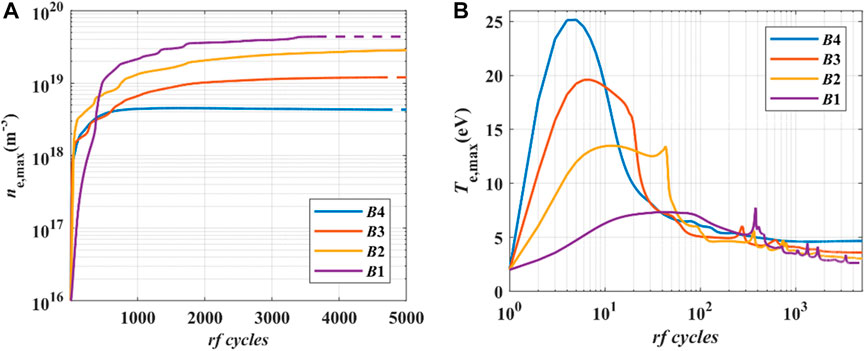
FIGURE 12. (A) Maximum electron density and (B) maximum electron temperature during the discharge with different magnetic fields.

Figure 13 shows the electron deposit power density at the steady state with different magnetic fields. When the magnetic field intensity of the uniform section is 0.005T, the configuration of deposit power density in Figure 13A is similar with that of the ICP source shown in Figure 7. As the magnetic field gets stronger, the deposit power density inside the plasma gradually increases.

FIGURE 13

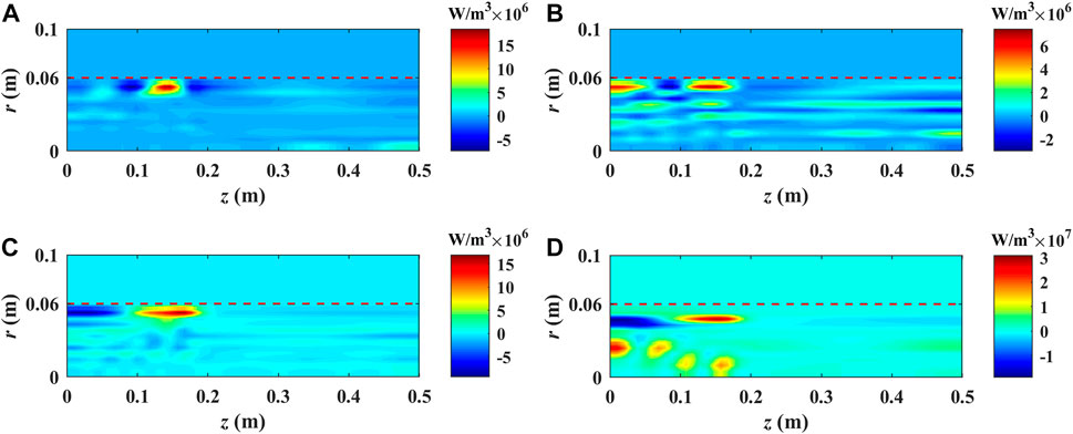
FIGURE 13. Deposit power density of electrons with different magnetic fields: (A) B4, (B) B3, (C) B2, and (D) B1.

Figure 14 shows the deposit power density with different magnetic fields at z = 0.15 m. Taking Figure 14A as an example, P_θ is 72% of P_total at r = 0.055 m and 89% of P_total at r = 0.05 m, which means the deposit power mainly comes from the θ-direction. Figure 7 and Figure 14A show that the helicon plasma source in the magnetic field B4 is in the H mode.

FIGURE 14

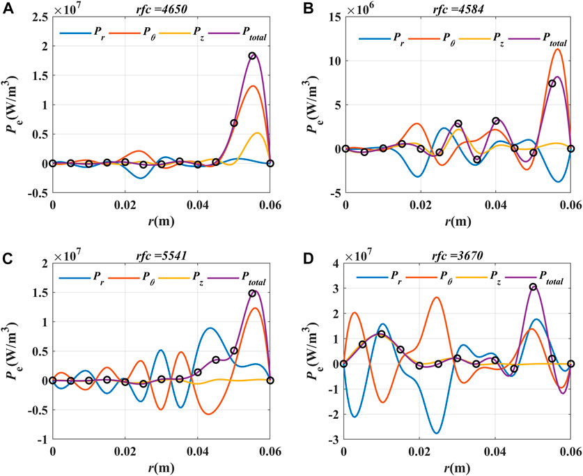
FIGURE 14. Deposit power density with different magnetic fields at z = 0.15m: (A) B4, (B) B3, (C) B2, and (D) B1.

The results of the simulation with different magnetic fields show how the power is deposited in the helicon plasma source. In the H mode and low-order wave mode, the deposit power density concentrates near the plasma edge and advances from the interaction between the electric field and electrons in the direction perpendicular with the magnetic field, while in the high-order wave mode, due to the resonance between the electric field and electrons, the deposit power density inside the plasma increases dramatically and it mainly comes from the parallel direction. For such mechanisms, the plasma density becomes much higher once the helicon plasma source converts to the high-order wave mode.

5 Summary and discussion

In this paper, a multi-fluid, two-dimensional, axisymmetric model coupled with the electromagnetic field was developed for the helicon plasma source in the MPRE, and the simulation with different magnetic fields was performed. The mechanism of mode conversion and power deposition in the helicon plasma source was analyzed.

During simulation, the operation mode continuously changes with time until the helicon plasma source becomes steady. Every time the mode changes, the electron temperature peak appears and leads to the dramatic increase of plasma density. In the high-order wave mode, the resonance between the electric field and electrons is observed. As a result of the resonance, the deposit power density inside the plasma significantly increases , and it mainly comes from the direction parallel with the magnetic field, while the deposit power density perpendicular to the magnetic field cancels out with each other.

When the magnetic field intensity increases, the operation mode gradually changes from the H mode to the high-order wave mode and the plasma density significantly increases. In other words, the ionization rate of the working medium can be much higher if the magnetic field is stronger, while the input power and the flow rate of the engine remain unchanged. As a result, more ions can be heated by the ICRH stage and the thrust together with the efficiency of the engine becomes higher.

In the helicon plasma source, not only the strength of magnetic field but also the input power and the flow rate of the working medium have an influence on the operation mode. In the future work, more simulations will be carried out with the model developed in this paper to gain a more comprehensive understanding of the helicon plasma source in the MPRE. To simplify the simulation, the axisymmetric model is adopted in this paper. However, whether the electromagnetic field of the helicon wave is axisymmetric requires further study. Therefore, the model in this paper needs to be expanded to 3D for a more precise description of the helicon wave.

Data availability statement

The original contributions presented in the study are included in the article/Supplementary Material, further inquiries can be directed to the corresponding author.

Author contributions

ZY carried out the multi-component fluid modeling. WF, XH, and CT analyzed the results of the simulation. All authors contributed to the article and approved the submitted version.

Funding

This work was supported by the Shaanxi Key Laboratory of Plasma Physics and Applied Technology. The content of this manuscript was presented in part at the 17th China Electric Propulsion Conference, Zhenyu Yang et al 2022, Plasma Sci. Technol., 24 074006.

Conflict of interest

The authors declare that the research was conducted in the absence of any commercial or financial relationships that could be construed as a potential conflict of interest.

Publisher’s note

All claims expressed in this article are solely those of the authors and do not necessarily represent those of their affiliated organizations, or those of the publisher, the editors, and the reviewers. Any product that may be evaluated in this article, or claim that may be made by its manufacturer, is not guaranteed or endorsed by the publisher.

References

1. Chang FR. Recent progress on the VASIMR Engine.IEPC-2022-525 (2022). Available at:https://ntrs.nasa.gov/citations/20050217236 (Accessed January 1, 2004).

Google Scholar

2. Squire JP, Carter M, Chang FR, Corrigan A, Dean L, Farrias J, et al. Run-time accumulation testing of the100kW VASIMR VX-200SS device. Cincinnati, Ohio: AIAAPaper (2018). p. 2018–4416.

Google Scholar

3. Chen FF, Torreblanca H. Large-area helicon plasma source with permanent magnets. Plasma Phys Control Fusion (2007) 49:81–93. doi:10.1088/0741-3335/49/5a/s07

CrossRef Full Text | Google Scholar

4. Charles C. Helicon double layer thruster. Sacramento, California: AIAAPaper (2006). p. 2006–4838.

Google Scholar

5. Cichocki F, Navarro-Cavallé J, Modesti A, Ramírez Vázquez G. Magnetic nozzle and RPA simulations vs. Experiments for a helicon plasma thruster plume. Front Phys (2022) 10:876684. doi:10.3389/fphy.2022.876684

CrossRef Full Text | Google Scholar

6. Del Valle JI, Chang Diaz FR, Granados VH. Plasma-Surface interactions within helicon plasma sources. Front Phys (2022) 10:856221. doi:10.3389/fphy.2022.856221

CrossRef Full Text | Google Scholar

7. Boswell RW. Plasma production using a standing helicon wave. Phys Lett (1970) 33A:457–8. doi:10.1016/0375-9601(70)90606-7

CrossRef Full Text | Google Scholar

8. Chen FF. Plasma ionization by helicon waves. Plasma Phys Controlled Fusion (1991) 33:339–64. doi:10.1088/0741-3335/33/4/006

CrossRef Full Text | Google Scholar

9. Chen FF, Blackwell DD. Upper limit to Landau damping in helicon discharges. Phys Rev Lett (1999) 82:2677–80. doi:10.1103/physrevlett.82.2677

CrossRef Full Text | Google Scholar

10. Blackwell DD, Chen FF. Time-resolved measurements of the electron energy distribution function in a helicon plasma. Plasma Sourc Sci Tech (2001) 10:226–35. doi:10.1088/0963-0252/10/2/312

CrossRef Full Text | Google Scholar

11. Boswell RW. Effect of boundary conditions on radial mode structure of whistlers. J.Plasma Phys (1984) 31:197–208. doi:10.1017/s0022377800001550

CrossRef Full Text | Google Scholar

12. Shamrai KP, Taranov VB. Volume and surface rf powerabsorption in a helicon plasma source. Plasma Sourc Sci. Technol. (1996) 5:474–91. doi:10.1088/0963-0252/5/3/015

CrossRef Full Text | Google Scholar

13. Cho S. The field and power absorption profiles in helicon plasma resonators. Phys Plasmas (1996) 3:4268–75. doi:10.1063/1.871556

CrossRef Full Text | Google Scholar

14. Blackwell DD, Madziwa TG, Arnush D, Chen FF. Evidence for trivelpiece-gould modes in a helicon discharge. Phys Rev Lett (2002) 88:145002. doi:10.1103/physrevlett.88.145002

PubMed Abstract | CrossRef Full Text | Google Scholar

15. Duan ZP, Yiwen L, Bailing Z, Lei Z, Weizhao Z. Numerical simulation on coupling mode of helicon wave and TG wave in magnetic field. J Propulsion Tech (2018) 39:1897.

Google Scholar

16. Li WQ, Zhao B, Wang G, Xiang D. Parametric analysis of mode coupling and liner energy deposition properties of helicon and Trivelpiece-Gould waves in helicon plasma. Acta Phys Sin (2020) 69:115201. doi:10.7498/aps.69.20200062

CrossRef Full Text | Google Scholar

17. Ellingboe AR, Boswell RW. Capacitive, inductive and helicon-wave modes of operation of a helicon plasma source. Phys Plasmas (1996) 3:2797–804. doi:10.1063/1.871713

CrossRef Full Text | Google Scholar

18. Shamrai KP. Stable modes and abrupt density jumps in a helicon plasma source. Plasma Sourc Sci. Technol. (1998) 7:499–511. doi:10.1088/0963-0252/7/4/008

CrossRef Full Text | Google Scholar

19. Chen FF, Torreblanca H. Density jump in helicon discharges. Plasma Sourc Sci. Technol. (2007) 16:593–6. doi:10.1088/0963-0252/16/3/019

CrossRef Full Text | Google Scholar

20. Kim SH, Hwang YS. Collisional power absorption near mode conversion surface in helicon plasmas. Plasma Phys Control Fusion (2008) 50:035007. doi:10.1088/0741-3335/50/3/035007

CrossRef Full Text | Google Scholar

21. Wu M, Xiao C, Wang X, Liu Y, Xu M, Tan C, et al. Relationship of mode transitions and standing waves in helicon plasmas. Plasma Sci Technol (2022) 24:055002. doi:10.1088/2058-6272/ac567d

CrossRef Full Text | Google Scholar

22. Yang Z, Xiao C, Liu Y, Yang X, Wang X, Tan C, et al. Effects of magnetic field on electron power absorption in helicon fluid simulation. Plasma Sci Technol (2022) 23:085002. doi:10.1088/2058-6272/ac0718

CrossRef Full Text | Google Scholar

23. Yang X, Cheng M-S, Wang MG, Li X-K. Three-dimensional direct numerical simulation of helicon discharge. Acta Phys Sin (2017) 2:025201. doi:10.7498/aps.66.025201

CrossRef Full Text | Google Scholar

24. Ventzek PLG, Hoekstra RJ, Kushner MJ. Two-dimensional modeling of high plasma density inductively coupled sources for materials processing. J Vacuum Sci Tech B (1994) 12:461. doi:10.1116/1.587101

CrossRef Full Text | Google Scholar

25. Zheng FH, Chen Z, Zhang J. Toward development of a three dimensional unconditionally stable finite-difference time-domain method. IEEE Trans Microwave Theor Tech (2000) 48:1550. doi:10.1109/22.869007

CrossRef Full Text | Google Scholar

26. Boris JP, Landsberg AM, Oran ES, Gardner JH. Lcpfct - a flux-corrected Transport algorithm for solving generalize d continuity equations. No.6410-93-7192. Washington DC: U.S. Naval Research Laboratory (1993).

CrossRef Full Text | Google Scholar

27. Wu M, Xiao C, Wang X, Liu Y, Xu M, Tan C, et al. Relationship of mode transitions and standing waves in helicon plasmas. Plasma Sci Technol (2021) 24:055002. doi:10.1088/2058-6272/ac567d

CrossRef Full Text | Google Scholar

28. Chi KK, Sheridan TE, Boswell RW. Resonant cavity modes of a bounded helicon discharge. Plasma Sourc Sci. Technol. (1999) 8:421–31. doi:10.1088/0963-0252/8/3/312

CrossRef Full Text | Google Scholar

29. Sun B, Zhao Y, Wei J, Fang J, Tan C. Plasma diagnostics of a high power helicon source. J Propulsion Tech (2019) 40:708.

Google Scholar