Abstract
Information geometry and Markov chains are two powerful tools used in modern fields such as finance, physics, computer science, and epidemiology. In this survey, we explore their intersection, focusing on the theoretical framework. We attempt to provide a self-contained treatment of the foundations without requiring a solid background in differential geometry. We present the core concepts of information geometry of Markov chains, including information projections and the pivotal information geometric construction of Nagaoka. We then delve into recent advances in the field, such as geometric structures arising from time reversibility, lumpability of Markov chains, or tree models. Finally, we highlight practical applications of this framework, such as parameter estimation, hypothesis testing, large deviation theory, and the maximum entropy principle.
1 Introduction
Markov chains are stochastic models that describe the probabilistic evolution of a system over time and have been successfully used in a wide variety of fields, including physics, engineering, and computer science. Conversely, information geometry is a mathematical framework that provides a geometric interpretation of probability distributions and their properties, with applications in diverse areas such as statistics, machine learning, and neuroscience. By combining the insights and methods from both fields, researchers have, in recent years, developed novel approaches for analyzing and modeling systems with time dependencies.
1.1 Outline and scope
As the fields of information geometry and Markov chains are broad, it is not possible to review all topics exhaustively, and we had to confine the scope of our survey to certain basic topics. Our focus will be on time-discrete, time-homogeneous Markov chains that take values from a finite alphabet. In particular, we will not cover time-continuous Markov chains [1, 2] nor discuss quantum information geometry or hidden Markov models [3, 4]. Our introduction to information geometry in the distribution setting will be limited to the basics. For a more comprehensive treatment, we recommend referring to the monographs [5, 6].
This survey is structured into five sections.
Section 1 is a brief introduction that provides an outline, lists the main concepts and results found in this survey, and clarifies its scope.
In Section 2, we lay out the notation that will be used throughout this paper and provide a primer on irreducible Markov chains and information geometry in the context of distributions. Along the way, we recall how to extend notions of entropy and Kullback–Leibler (KL) divergence from distributions to Markov chains.
In Section 3, following Nagaoka [7], we introduce a Fisher metric and a pair of dual affine connections on the set of irreducible stochastic matrices, which allows us to define the orthogonality of curves and parallel transport. We then proceed to define exponential families (e-families) and mixture families (m-families) of Markov chains. Importantly, the set of irreducible stochastic matrices is shown to form both an e-family and m-family, endowing it with the structure of a dually flat manifold. We explore minimality conditions for exponential families and chart transition maps between their natural and expectation parameters. Additionally, we define geodesics and their generalizations and conclude the section with a discussion on information projections and decomposition theorems. Specifically, similar to the distribution setting, the dual affine connections induce two notions of convexity, leading to Pythagorean identities.
In Section 4, we explore some recent developments in the field. First, we list and analyze the geometric properties of important subfamilies of stochastic matrices, such as symmetric or bistochastic Markov chains. The highlights of this section include the analysis of geometric properties induced by the time reversibility of Markov chains. This analysis leads to the establishment of the em-family structure of the reversible set, the derivation of closed-form expressions for reversible information projections, and the characterization of the reversible set as geodesic hulls of contained families. We continue this section by discussing some notable advancements in the context of data processing of Markov chains. Mirroring congruent embeddings in a distribution setting, we present a construction of embeddings of families of stochastic matrices that are congruent with respect to the lumping operation of Markov chains. These embeddings preserve the Fisher metric, the pair of dual affine connections, and the e-family structure. Additionally, we explore the establishment of a foliation structure on the manifold of lumpable stochastic matrices. Lastly, we conclude this section by presenting results in the context of tree models.
Section 5 is devoted to applications of the information geometry framework to large deviations, estimation theory, hypothesis testing, and the maximum entropy principle.
2 Preliminaries
2.1 Notation
Let be a finite space of symbols. All vectors will be written as row vectors. A vector is non-negative (resp., positive), indicated by v ≥ 0 (resp., v > 0), when v(x) ≥ 0 (resp., v(x) > 0) for any . For , the vector is defined by for , where is the function that takes the value 1 when the predicate in the argument is true and 0 otherwise. For two vectors , the Hadamard product of u and v is defined by (u∘v)(x) = u(x)v(x), and we will also use the shorthand (u/v)(x) = u(x)/v(x). For convenience, for k vectors u1, …, uk, we write , and for vector u and positive real number α, u∘α is such that u∘α(x) = u(x)α. For p ≥ 0, we write . We denote by the set of all distributions over ,and refers to the positive subset. X ∼ μ means that the random variable X is distributed according to a distribution , and for , the absolute continuity of ν with respect to μ is denoted by ν ≪ μ.
2.2 Irreducible Markov chains
A time-discrete, time-homogeneous Markov chain is a random process that takes values on the state space and satisfies the Markov property. Namely, for t ≥ 2 and for any ,with for an initial distribution . The transition probabilities of the process can be organized in a row-stochastic matrix P, where . We write X ∼ (μ, P) for the Markov chain started from μ and with transition matrix P. Let the vector space , whose elements can be conveniently represented by real square matrices of size , simultaneously understood as linear operators on . We introduce the set of all row-stochastic matrices over the space ,As we assume , for any member P of , there exists a fixed point such that πP = π, and we call π a stationary distribution for P. Let define the set of positive probability transitions on the state space. When is a fully connected digraph, we say that P is irreducible. Algebraically, this means that for any pair of states , there exists such that Pp(x, x′) > 0, or less tersely, there exists a path on the graph from x to x′. When P defines an irreducible Markov chain, the stationary distribution π is unique and positive. Moreover, when the initial distribution μ = π, we say that the chain is stationary, write for probability statements over a stationary trajectory and X ∼ P as a shorthand for X ∼ (π, P). We denote the irreducible set:
It will also be convenient to define , the real functions over , and identify this set with all functions over that are null outside of . Note that can be endowed with the structure of a -dimensional vector space. We write for the positive subset. For , the probability of observing a stationary path x1 → x2 → ⋯ → xn induced from a π-stationary P is given by
In particular,is called the edge measure pertaining to P. Observe that the map from an irreducible transition matrix P to its edge measure is one-to-one (see, e.g., [8]) and that the set of all edge measures can be expressed as
We refer the reader to Levin et al. [9] for a thorough treatment of Markov chains.
2.3 Entropy and divergence rates for Markov chains
Let us first recall the definition of the Shannon entropy of a random variable. We let and X ∼ μ. The entropy H of the random variable X, which measures the average level of surprise inherent to the possible outcomes, is defined byand where by convention 0 log 0 = 0. The entropy rate of a stationary stochastic process corresponds to the number of bits to describe one random variable in a stochastic process averaged over time. Namely,where for any , H(X1, X2, …, Xn) is the joint entropy of the random variables X1, X2, …, Xn. Particularly, when X forms an irreducible Markov chain with transition matrix and stationary distribution π, the entropy rate can be written aswhere Q is the edge measure pertaining to P. In other words, the entropy rate of the process is computed from P only. We can thus overload H to define
For two random variables X ∼ μ, X′ ∼ μ′ with , we define the Kullback–Leibler divergence from X′ to X by
Extending the aforementioned definition to Markov processes, the information divergence rate [10] (see also [73, Section 3.5]) of , from another chain , is given bywhich is also agnostic on initial distributions, inviting us to lift the definition of D to stochastic matrices:
2.4 Information geometry
We briefly introduce basic concepts related to information geometry in the context of distributions. The central idea is to regard as a -dimensional smooth manifold and statistical models, i.e., parametric families of distributions , as smooth submanifolds of . At each point , we define a (0,2)-tensor,where is the tangent plane at the point μ, and Uμ log μ(x) is the directional derivative of the function, μ↦ log μ(x) with respect to the tangent vector Uμ. This leads to the definition of a Riemannian metric, termed Fisher metric [5, Section 2.2]:where is the set of all vector fields [5, Section 1.3] and the set of all smooth real functions on . Letting be a chart map1, μθ denote the distribution at coordinates θ = (θ1, …, θd), and ∂i = ∂ ⋅/∂θi, we write for the θ-induced basis of . We can express the Fisher metric at coordinates θ as
In addition to , we define a pair of affine connections by their associated covariant derivatives [5, Chapter 1, (1.38)]:
In the parametrization θ, the connections are specified by their coefficients (Christoffel symbols):where is the covariant derivative of ∂j with respect to ∂i. The canonical divergence associated with and ∇(m) is the Kullback–Leibler divergence (5). The connections ∇(e) and ∇(m) are conjugate [5, Chapter 3, (3.1)] in the sense where for any vector fields ,
As a consequence, the curvature tensors associated with ∇(e), ∇(m) vanish simultaneously. In particular, they vanish for , and we say that the manifold is dually flat. A complete review of the distribution setting, including exponential and mixture families, is outside the scope of this survey. We refer the reader to Amari and Nagaoka [5] for a complete treatment of the topic.
3 The dually flat manifold of irreducible stochastic matrices
Similar to the distributional setting, we regard , the set of irreducible stochastic matrices over some prescribed fully connected digraph , as a smooth manifold, on which we introduce a Riemannian metric together with a dually flat structure (Section 2.3). In turn, we will define exponential and mixture families of stochastic matrices. We will further examine notions of geodesic convexity and information projections.
3.1 The information manifold
Our first order of business is to establish a dually flat structure on the set of stochastic matrices, following Nagaoka [7]. A smooth manifold structure can be established on , using the map introduced by Nagaoka [7, p.2], reported in (15). One possible construction is based on the definition of the informational divergence between two Markov processes at (6) and gives rise to a metric and dual affine connections [11, 12]. We proceed to confirm that while the structure can be defined without invoking asymptotic notions, the obtained Fisher metric and affine connections are indeed asymptotically consistent with their distributional counterparts for path measures.
3.1.1 Divergence as a general contrast function
Recall the definition of the information divergence from one stochastic matrix
to another
given at
(6). We henceforth focus on the setting where the supports are identical
; that is, stochastic matrices
P,
P′ belong to
and
. We are interested in parametric families of irreducible matrices. Namely, for some open and connected parameter space
, we define
and regard
as a smooth submanifold of
with a global coordinate system
θ. For
, for simplicity, let us write
θ= (
θ1,
…,
θd) =
θ(
P),
θ′ =
θ(
P′),
, and
and use the shorthand
. The information divergence rate
we defined in
(6)is
C3and satisfies the following properties of a contrast function:
(i) for any θ, θ′ ∈ Θ (non-negativity).
(ii) if and only if θ = θ′ (identity of indiscernibles).
(iii) for any i, j ∈ [d] (vanishing gradient on the diagonal).
(iv) is positive definite.
We callthe dual divergence of D.
3.1.2 Fisher metric and dual affine connections
From any divergence function D on a manifold verifying the aforementioned properties (i), (ii), (iii), and (iv), one can construct a conjugate connection manifold:where the Riemannian metric and Christoffel symbols of ∇ and ∇* are expressed in the chart and for any i, j, k ∈ [d] as
As the metric and connections are derived from the KL divergence, they all depend solely on the transition matrices and are, in particular, agnostic of initial distributions. From calculations, we obtain the Fisher metric [7, (9)]:and the coefficients for the pair of torsion-free affine connections ∇(e) (e-connection) and ∇(m) (m-connection) [7, (19, 20)]:
On the one hand, the metric encodes notions of distance and angles on the manifold. In particular, the information divergence D locally corresponds to the Fisher metric. In other words, for and such that θ + δθ ∈ Θ,
Consider two curves , and suppose that they intersect at some point , achieved without loss of generality at γ(0) and σ(0). We define the angle between the curves γ and σ at P0 as the angle formed by the two curves in the tangent space at P0: and we will say that the two curves are orthogonal at P0 when the inner product is null. On the other hand, affine connections define notions of straightness on the manifold. The fact that the connections are coupled with the metric introduces a generalization of the invariance of the inner product under the parallel translation of Euclidean geometry. Letting denote parallel translations along a curve γ from P to P′ with respect to ∇(e) and ∇(m), for any ,
3.1.3 Asymptotic consistency with information rates
Recall from (2) that a stationary Markovian trajectory has a probability described by the path measure Q(n). For every , one can consider the manifold of all path measures of length n. Computing the limit of the metric and connection coefficients [7, 13],where , ∇[n],(e), and ∇[n],(m) are the Fisher metric and e/m-connections on , with . Therefore, the Fisher metric for stochastic matrices essentially corresponds to the time density of the average Fisher metric, and a similar interpretation can be proposed for the affine connections.
3.2 Exponential families and mixture families
Similar to the distribution setting, we proceed to define exponential families (e-families) and mixture families (m-families) of stochastic matrices.
3.2.1 Definition of exponential families
Definition 3.1(e-family of stochastic matrices [7]). Let. We say that the parametric family of stochastic matricesis an exponential family (e-family) of stochastic matrices with natural parameterθ, when there exist functionsand, such that, for anyandθ ∈ Θ,For some fixedθ ∈ Θ, we may write for convenienceψθforψ(θ) andRθfor.
Note that R and ψ are analytic functions of θ and that ψ is a convex potential function. R and ψ are completely determined from g1, …, gd and K by the Perron–Frobenius (PF) theory, and we can introduce a stochastic rescaling mapping [7, 13]:where ρ and v are, respectively, the PF root and right PF eigenvector of . Following this notation, we can rewrite Definition 3.1 more simply aswhere exp is understood to be entry-wise. In particular, forms an e-family. Indeed, with and in the parametrization proposed by Ito and Amari [14], we pick an arbitrary and write
The basis is given byand the parameters are
We can alternatively define e-families as e-autoparallel submanifolds of [7, Theorem 6], where a submanifold is said to be autoparallel with respect to an affine connection ∇ when for any , it holds that .
3.2.2 Affine structures and characterization of minimal exponential families
We define the set of functions [7, 13, 15]and observe that we can endow with the structure of a -dimensional vector subspace of the -dimensional space . We can thus define the quotient space of generatorsof dimension and the diffeomorphismwhere ∘ stands here for function composition. Essentially, there is a one-to-one correspondence between vector subspaces of and e-families.
([7, Theorem 2]). A submanifoldforms an e-family if and only if there exists an affine subspacesuch that. In this case,.
As a corollary [7, Corollary 1], is trivially an exponential family of dimension . A family will be called minimal (or full) whenever the functions g1, …, gd in Definition 3.1 are linearly independent in . In this case, we will say that g1, …, gd form a basis for .
3.2.3 Mixture families
In the stochastic matrix setting, the notion of a mixture family is naturally defined in terms of edge measures.
Definition 3.2(m-family of stochastic matrices [15]). We say that a family of irreducible stochastic matricesis a mixture family (m-family) of irreducible stochastic matrices onwhen the following holds.There exists affinely independent, andwhere, andQξis the edge measure that pertains toPξ. Note that Ξ is an open set,ξis called the mixture parameter, anddis the dimension2of the family.
It is easy to verify that also forms an m-family, and it is possible to define m-families as m-autoparallel submanifolds of .
3.2.4 Dual expectation parameter and chart transition maps
For an exponential family with natural parametrization [θi], following Definition 3.1, one may introduce [7] the expectation parameter [ηi] as follows. For i ∈ [d] and θ ∈ Θ,where Qθ is the edge measure corresponding to the stochastic matrix at coordinates θ. When is minimal, η defines an alternative coordinate system to the natural parametrization θ for .
, Lemma 4.1
] The following statements are equivalent:(i) The functionsg1, …, gdare linearly independent in.
(ii) The mappingsθ∘η−1andη∘θ−1are one-to-one.
(iii) The Hessian matrixfor anyθ ∈ Θ.
(iv) The Hessian matrixforθ = 0.
(v) The parametrizationis faithful.
Defining the Shannon negentropy3 potential function to satisfywe can express [7, Theorem 4] the chart transition maps (see Figure 1) between the expectation [ηi] and natural [θi] parameters of the e-family aswhere we wrote ∂i⋅ = ∂ ⋅/∂ηi. We can also obtain the counterpart [13, Lemma 5] of (16) for θ◦η−1,
FIGURE 1

Natural and expectation parametrizations of an e-family , together with their chart transition maps.
3.2.5 Dual flatness
A straightforward computation shows that all the e-connection coefficients for an e-family and all the m-connection coefficients for an m-family are null. We say that is e-flat and that is m-flat. From the conjugacy of the affine connections, curvature tensors associated with ∇(e) and ∇(m) vanish simultaneously. As a consequence, for any smooth submanifold ,which is sometimes called the fundamental theorem of information geometry [79, Theorem 3]. In other words, e-families and m-families are both e-flat and m-flat [7, Theorem 5], and for any , it is enough to find an affine coordinate system in which either the e-connection or m-connection coefficients are null for it to be dually flat. For i, j ∈ [d], recall that . Similarly, we define . The coefficients of the Fisher metric and its inverse are recovered byThus, φ is also strictly convex, and the coordinate systems [θi] and [ηi] are mutually dual with respect to . The two coordinate systems are related by the Legendre transformation, and we can express their dual potential functions as
3.2.6 Geodesics and geodesic hulls
An affine connection ∇ defines a notion of the straightness of curves. Namely, a curve γ is called a ∇-geodesic whenever it is ∇-autoparallel, , where is the velocity vector at time parameter t. The geodesic between two points is the straight curve that goes through the two points. As our manifold is equipped with two dual connections, there are two distinct notions of straight lines, and the arc between the two points will not necessarily correspond to the shortest path between the two elements with respect to the Riemannian metric, unlike in Euclidean geometry. Specifically, the e-geodesic going through P0 and P1 is given [7, Corollary 2] byand the m-geodesic [7, Theorem 7] bywhere is the set of all edge measures introduced in (3). A submanifold forms an e-family if and only if for any two points , lies entirely in [7, Corollary 3], and a similar claim holds for m-families. We generalize the aforementioned objects beyond two points to more general subsets of , by defining geodesic hulls [13] (see Figure 2).
FIGURE 2

E-hull of three points. It is instructive to note that although a set of three points forms a zero-dimensional manifold, we construct a manifold of dimensions possibly up to two.
Definition 3.3(Exponential hull [13, Definition 7]). Let:whereis defined in (12).
Definition 3.4(Mixture hull [13, Definition 8]). Let:whereQ(resp.,Qi) is the edge measure that pertains toP(resp.,Pi).
When a family forms both an m-family and an e-family, we say it forms an em-family.
3.3 Information projections and decomposition theorems
The projection of a point onto a surface is among the most natural geometric concepts. In Euclidean geometry, projecting on a connected convex body leads to a unique closest solution point. However, the dually flat geometry on is based on two different notions of straightness, inducing two different flavors of geodesic convexity. Furthermore, the divergence function we consider is not symmetric in its arguments, hence the need for two definitions of projections as minimizer with respect to the first and second arguments. This section goes back to and hinges around the notion of divergence defined in (6), projection, and orthogonality and explores the Bregman geometry of .
3.3.1 Information divergence as a Bregman divergence
For a continuously differentiable and strictly convex function on a convex domain , we call Bregman divergence Bf [16] with generator f (see Figure 3) the function
FIGURE 3

Geometrical interpretation of a Bregman divergence.
When we let some e-family following Definition 3.1, one can verify with direct computations [15, 17] that
As ψ and φ are convex conjugate,where we used the shorthands η = η(θ) and η′ = η(θ′); hence, the KL divergence is the Bregman divergence associated with the Shannon negentropy function, and as any Bregman divergence, it verifies the law of cosines:which can be re-expressed [7, (23)] asfor γ an m-geodesic going through Pθ and Pθ′ and σ an e-geodesic going through Pθ′ and Pθ″.
3.3.2 Canonical divergence
One may naturally wonder whether it is possible to recover the divergence D defined at (6) from and ∇(e), ∇(m) only. This is referred to as the inverse problem in information geometry. It is easily understood that such a divergence is not unique. In fact, there exist an infinity of divergence functions that could have given rise to the dually flat geometry on [18]. However, it is possible to single out one particular divergence, termed canonical divergence [5], which is uniquely defined from and ∇(e), ∇(m). For , its expression is given in a dual coordinate system [θi], [ηi] bywhere η = η(P) and θ′ = θ(P′). One can verify from (21) that we indeed recover the expression at (6).
3.3.3 Geodesic convexity and convexity properties of information divergence
Geodesic convexity is a natural generalization of convexity in Euclidean geometry for subsets of Riemannian manifolds and functions defined on them. As straight lines are defined with respect to an affine connection ∇, a subset of is said to be geodesically convex with respect to ∇ when ∇-geodesic joining4 two points in remain in at all times. In particular, is e-convex (resp., m-convex), when for any and any t ∈ [0, 1], it holds that (resp., ), where and are defined in (19, 20). An immediate consequence is that an e-family (resp., m-family) is e-convex (resp., m-convex). On a geodesically convex domain , a function is said to be a geodesically convex (resp., strictly geodesically convex) if the composition is a convex (resp., strictly convex) function for any geodesic contained within . In particular, the information divergence defined in (6) is strictly m-convex in its first argument and strictly e-convex in its second argument [15, Theorem 3.3]. Namely, for t ∈ (0,1), , with P0 ≠ P1,
However, for , the opposite inequality holds [13]:
Unlike in the distribution setting, where the KL divergence is jointly m-convex, this property does not hold true for stochastic matrices [21, Remark 4.2].
3.3.4 Pythagorean inequalities
In the more familiar Euclidean geometry, projecting a point P onto a subset of consists in finding the point in that minimizes the Euclidean distance between P and . If is convex, the minimization problem admits a unique solution and a Pythagorean inequality holds between the point, its projection, and any other point in . Similar ideas are made possible on by the Bregman geometry induced from D. Let (resp., ) with be non-empty, closed, and m-convex (resp., e-convex). We define the e-projection onto as the mappingand the m-projection onto as the mapping
For a point P in context, we simply write Pe = Pe(P) and Pm = Pm(P).
(Pythagorean inequalities for geodesic e-convex [
21, Proposition 4.2], m-convex sets [
23, Lemma 1]).
The following statements hold.(i) Peexists in the sense where the minimum is attained for a unique element in.
(ii) For,P0 = Peif and only if
(iii) Pmexists in the sense where the minimum is attained for a unique element in.
(iv) For,P0 = Pmif and only if
3.3.5 Pythagorean equality for linear families
Inequalities become equalities when projecting onto e-families and m-families.
(Pythagorean theorem for e-families, m-families [
19], [
15, Section 4.4]).
The following statements hold.(i) Peexists in the sense where the minimum is attained for a unique element in.
(ii) For,P0 = Peif and only if
(iii) Pmexists in the sense where the minimum is attained for a unique element in.
(iv) For,P0 = Pmif and only if
3.4 Bibliographical remarks
The construction of the conjugate connection manifold from a general contrast function in Section 3.1.1 and Section 3.1.2 follows the general scheme of Eguchi [11, 12], which can also be found in [79, Definition 5, Theorem 4]. The expression for the Fisher metric at (Eq. 8) and the conjugate affine connections at (Eq. 8) were introduced by Nagaoka [7, (9), (19), (20)]. One-dimensional e-families of stochastic matrices were first introduced by Nakagawa and Kanaya [19], whereas the general construction in the multi-dimensional setting was done by Nagaoka [7], who also established the characterization in Theorem 3.1 of minimal e-families in terms of affine structures of in [7, Theorem 2]. Curved exponential families of transition matrices and mixture families make their first named appearances in Hayashi and Watanabe [15; Section 8.3; Section 4.2]. See also [13, Definition 1] for two alternative equivalent definitions of an m-family. The expectation parameter for exponential families in (16) and its expression as the gradient of the potential function were discussed on multiple occasions [7, Theorem 4], [19, (28)], [15, Lemma 5.1]. Theorem 3.2 was taken from [15, Lemma 4.1]. The expression for the chart transition map from expectation to natural parameters in (17) was obtained from [13, Lemma 5]. Geodesics discussed in Section 3.2.6 were introduced in one-dimension in [19] and multiple dimensions in [7], whereas mixture and exponential hulls of sets first appeared in [13]. Nagaoka [7] established the dual flatness of the manifold discussed in Section 3.2.5 and matched the information divergence with the canonical divergence. The expression of the informational divergence and entropy for exponential families in (21) was given in [15, 17]. The law of cosines was also mentioned by Adamčík [20] for general Bregman projections. The convexity properties of the divergence appeared in Hayashi and Watanabe [15, Theorem 3.3] and Hayashi and Watanabe [15, Lemma 4.5], and their strict version was discussed in [21, Section 4] together with the case . The Pythagorean inequality for projections onto m-convex sets [Theorem 3.3 (i), (ii)] was shown to hold by Csiszár et al. [23, Lemma 1]. The inequality for the “reversed projection” onto e-convex sets was found in [21]. The equality in the Pythagorean theorem for e-families and m-families was first found in [19, Lemma 5] for the one-dimensional setting and in [15, Corollary 4.7, Corollary 4.8] for multiple dimensions.
3.4.1 Timeline
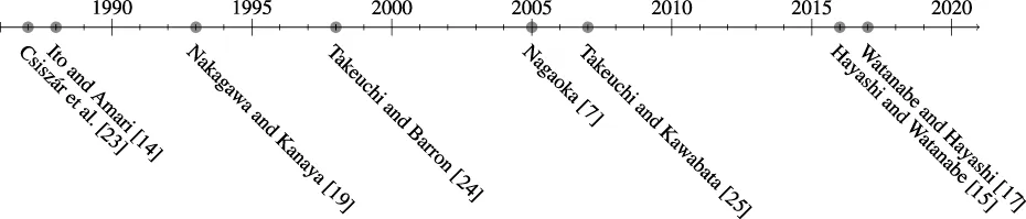
The idea of tilting or exponential change of measure, which gives rise to e-families in the context of distributions, can be traced back to Miller [22]. However, in this section, we focused on the milestones toward the geometric construction of Nagaoka [7], and we deferred the history of the development of the large deviation theory to Section 5.2. The first to recognize the exponential family structure of stochastic matrices is Csiszár et al. [23] by considering information projections onto linearly constrained sets and inferring exponential families as the solution to the maximum entropy problem, as discussed in more detail in Section 5.1. The notion of an asymptotic exponential family was implicitly described by Ito and Amari [14] and was formalized by Takeuchi and Barron [24] and Takeuchi and Kawabata [25]. A later result by Takeuchi and Nagaoka [26] proved that asymptotic exponential families and their non-asymptotic counterparts are in fact equivalent.
3.4.2 Alternative constructions
Some alternative definitions of exponential families of Markov chains include [27–32]. However, they do not enjoy the same geometric properties as the one of Definition 3.1. Thus, we do not discuss them in detail.
4 Recent advances
One area of recent progress has been the analysis of the geometric properties of significant submanifolds of . In Section 4.1, we briefly discuss symmetric, bistochastic, and memoryless classes. In Section 4.2, we turn the spotlight onto the structure-rich family of irreducible and reversible stochastic matrices. In Section 4.3, we mention some recent progress in connecting the dually flat geometry of Section 3.1 to the theory of lumpability of Markov chains. We end with a discussion on finite state machine (FSMX) models in Section 4.4.
4.1 Symmetric, bistochastic, and memoryless stochastic matrices
In this section, we briefly survey known geometric properties of notable submanifolds of . We also refer the reader to Table 1, adapted from [13, Table 1], for a more visual classification.
TABLE 1
| Manifold | m-family | e-family | Dimension |
|---|---|---|---|
| Yes | Yes | ||
| Yes | Yes | ||
| Yes | Yes | ||
| Yes | No | ||
| Yes | No | ||
| No | Yes |
Geometry of submanifolds of irreducible Markov kernels for .
4.1.1 Memoryless class
We say that a stochastic matrix is memoryless, when it can be expressed asfor . We note that π is the stationary distribution of P, and that for such P to be irreducible, it is necessary that π > 0; hence, . Markov chains defined by a memoryless stochastic matrix correspond in fact to an iid process. We write for the set of all memoryless stochastic matrices.
Lemma 4.1
([
13, Lemma 7, Lemma 8]).
The two following statements hold:(i) forms an e-family of dimension.
(ii) does not form an m-family.
Recall the parametrization of Ito and Amari [14], reported in (13). Coefficients θij in the expression represent memory in the process, and thus vanish. For and an arbitrary x* ∈ [m], we can re-writewhere for i ∈ [m], i ≠ x*,
4.1.2 Bistochastic class
Bistochastic matrices, also called doubly stochastic matrices, are row- and column-stochastic. In other words, is bistochastic if and only if the transposition . In particular, the stationary distribution of a bistochastic matrix is uniform. We denote as the set of positive bistochastic matrices.
Lemma 4.2
4.1.3 Symmetric class
A symmetric stochastic matrix P satisfies P(x, x′) = P(x′, x) for any pair of states . Writing for the set of positive symmetric matrices, note that lies at the intersection of reversible (see Section 4.2) and doubly stochastic matrices, enjoying all their properties (e.g., uniform stationary distribution, self-adjointness). However, perhaps surprisingly, does not form an e-family.
Lemma 4.3
([
13, Lemma 9, Lemma 10]).
The two following statements hold:(i) forms an m-family of dimension,
(ii) For,does not form an e-family.
4.2 Time-reversible stochastic matrices
In Section 4.2.1, we begin by briefly introducing time reversals and time reversibility in the context of Markov chains. In Section 4.2.2, we proceed to analyze geometric structures that are invariant under the time reversal operation. In Section 4.2.3, we inspect the e-family and m-family nature of the submanifold of reversible stochastic matrices and reversible edge measures. In Section 4.2.4 and Section 4.2.5, we, respectively, discuss reversible information projections and how to generate the reversible set as a geodesic hull of structured subfamilies.
4.2.1 Reversibility
Consider a Markov chain with transition matrix , started from its stationary distribution π. When we look at the random process in reverse time , the Markov property is still verified. In fact, the transition matrix P* of this time-reversed Markov chain is given by P*(x, x′) = π(x′)P(x′, x)/π(x). The time reversal P* shares the same stationary distribution as the original chain, and irreducibility is preserved, although , where is the symmetric image of the connection digraph . When P* = P, the transition probabilities of the chain forward and backward in time coincide, and we say that the chain is time-reversible. Equivalently, we may say that P verifies the detailed balance equation:
We write for the set of reversible chains that are irreducible with connection digraph . Note that the edge set must necessarily satisfy ; otherwise, .
Time-reversibility is a central concept across a myriad of scientific fields, from computer science (queuing networks [33], storage models, Markov Chain Monte Carlo algorithms [34], etc.) to physics (many classical or quantum natural laws appear as being time-reversible [35]). The theory of reversibility for Markov chains was originally developed by Kolmogorov [36, 37], and we refer the reader to [38] for a more complete historical exposition.
Reversible Markov chains enjoy a particularly rich mathematical structure. Perhaps first and foremost, reversibility implies self-adjointness of P with respect to the Hilbert space ℓ2(π) of real functions over endowed with the weighted inner product . Key properties of reversible stochastic matrices induced from self-adjointness include a real spectrum, control from above and below the mixing time by the inverse of the absolute spectral gap [9, Chapter 12], and stability of spectrum estimation procedures [39]. Reversibility has also been explored in the context of algebraic statistics [40] or Bayesian statistics [41]. In this section, we focus on the properties of reversibility and families of reversible stochastic matrices from an information geometric viewpoint.
4.2.2 Geometric invariants
The time reversal operation is known to preserve some geometric properties of families of transition matrices. Consider , a family of irreducible stochastic matrices. The time-reversal family [13, Definition 3], denoted as , is defined by
Lemma 4.4([13, Proposition 1]). Let(resp.,) be an e-family (resp., m-family) in. Then,(resp.,) forms an e-family (resp., m-family) in.
Moreover, the time reversal operation leaves the divergence between stochastic matrices unchanged [80, Proof of Proposition 2]:
When , we say that the family is reversible, and in this case , with . From the definition of an e-family , it is possible to determine whether is reversible. It is convenient to first introduce the class of log-reversible functions [13, Definition 4, Corollary 1]:
Lemma 4.5([13, Theorem 2]). Letbe an e-family that follows the expression of (11). Thenif and only ifandand for alli ∈ [d],.
4.2.3 The em-family of reversible stochastic matrices
The class of functions introduced in (25) can be endowed with the structure of a vector space [13, Lemma 4], which verifies the following inclusions:where was defined in (14). Immediately, , and this enables us to further define the quotient space of reversible generators:
It is possible to verify thatwhere Δ is the diffeomorphism defined in (15). The following result is then a consequence of Theorem 3.1.
([13, Theorem 3, Theorem 5, Theorem 6]). forms an e-family and an m-family of dimensionwhereis the set of loops in the connection graph.
([13, Theorem 4, Theorem 5]). Let, with stationary distributionπ. Pick an arbitrary element, and define
For, the collection of functionsforms a basis for. We can writePas a member of the m-family of reversible stochastic matrices by expressing its edge measureQasand we can writePas a member of the e-family,when, andP(x, x′) = 0 otherwise.
4.2.4 Reversible information projections
Let with . We recall the definitions (see Section 3.3) of the m-projection Pm and the e-projection Pe of P onto ,
There are known closed-form expressions for Pm and Pe. Moreover, the fact that forms an em-family (Theorem 4.1) leads to a pair of Pythagorean inequalities (see Figure 4), and the invariance of D under time reversals highlighted in (24) implies a bisection property.
FIGURE 4

Information projections onto , and illustrations of Pythagorean identities and bisection property of Theorem 4.3.
([13, Theorem 7, Proposition 2]). Letwith:whereis defined in Eq. (12). Moreover, for any,PmandPesatisfy the following Pythagorean identities:
Furthermore, the following bisection property holds
Finally, we mention that the entropy production σ(P) for a Markov chain with transition matrix P, which plays a central role in discussing irreversible phenomena in non-equilibrium systems, can be expressed in terms of the canonical divergence [81, (22)] as follows:
4.2.5 Characterization of the reversible family as geodesic hulls
It is known that the set of bistochastic matrices—also known as the Birkhoff polytope—is the convex hull of the set of permutation matrices (theorem of Birkhoff and von Neumann [42–44]). By recalling from Section 3.2.6 the definition of geodesic hulls (Definition 3.3, Definition 3.4) of families of stochastic matrices, results in a similar spirit are known for generating the positive and reversible family as geodesic hulls of particular subfamilies.
([
13, Theorem 9, Theorem 10]).
It holds that(i)
(ii) For,5
.
4.3 Markov morphisms, lumping, and embeddings of Markov chains
In the context of distributions, Čencov [45] introduced Markov morphisms in an axiomatic manner as the natural mappings to consider for statistics. The Fisher information metric can then be characterized as the unique invariant metric tensor under Markov morphisms [45–47]. In the context of stochastic matrices, we saw that the metric and connections introduced in Section 3 were asymptotically consistent with Markov models. This section connects with the axiomatic approach of Čencov and proposes a class of data processing operations that are arguably natural in the Markov setting.
4.3.1 Lumpability
We briefly recall lumpability in the context of distributions and data processing. Consider a distribution , and let Y1, Y2, …, be a sequence of random variables independently sampled from μ. Suppose we define a deterministic, surjective map , where is a space not larger than , and we inspect the random process defined by . Note that κ induces a partition of the space , with . The new process is again a sequence of independent random variables sampled identically from the push-forward distribution κ(μ) = μ◦κ−1, where we used an overloaded definition . Namely, the probability of the realization is the probability of the preimage ; for ,
When , symbols are merely being permuted. As with any data-processing operation, monotonicity of information dictates that two distributions can only be brought closer together with respect to D by the action of κ:
Crucially, in the independent and identically distributed setting, the lumping operation can be understood both as a form of processing of the stream of observations and as an algebraic manipulation of the distribution that generated the random process.
For Markov chains, the concept of lumpability is vastly richer. The first fact one must come to terms with is that a Markov chain may lose its Markov property after a processing operation on the data stream [48, 49], even for an operation as basic as a lumping. A chain is said to be lumpable [50] with respect to a lumping map , when the Markov property is preserved for the lumped process.
([50, Theorem 6.3.2]). Let.Pis lumpable if and only if for alland for all, it holds that, where for,.
The subset of of all lumpable stochastic matrices is written . We overload the operation and the κ-lumped stochastic matrix is denoted as κ(P) with, for any ,
4.3.2 Embeddings of Markov chains
Embeddings of stochastic matrices that correspond to conditional models were proposed and analyzed in [
51–
53]. However, the question of Markov chains, where one considers the stochastic process, was only recently explored in [
21]. Looking at reverse operations to lumping, we are interested in embedding an irreducible family of chains
into a space of irreducible chains
defined on a larger state space
, with some compatible edge set
. In [
21], it is postulated that natural morphisms should satisfy the following requirements:
A.1 Morphisms should preserve the Markov property.
A.2 Morphisms should be expressible as algebraic operations on stochastic matrices.
A.3 Morphisms should have operational meaning on trajectories of observations.
The following definition of a Markov morphism was proposed in [21].
Definition 4.1(Markov morphism for stochastic matrices [21, Definition 3.2]). A mapis called aκ-compatible Markov morphism for stochastic matrices when for any,where, and for any, it holds that
The constraints on the function Λ in Definition 4.1 ensure that the objects produced by λ are stochastic matrices and are κ-lumpable. Furthermore, given the full description of P and Λ, one can directly compute the embedded λ(P), thereby satisfying A.1 and A.2. Alternatively, when given a sequence of observations and without even knowing P, one can apply a random mapping ϕΛ on the trajectory and simulate a trajectory generated from the embedded chain, essentially satisfying axiom A.3. A key feature of a Markov morphism λ is that the divergence between two points and their image is unchanged [21, Lemma 3.1]. Namely, for two points ,
As a consequence, the Fisher metric and affine connections are preserved [21, Lemma 3.1] (see Figure 5), in the sense where for ,and for any vector fields ,wheredefined by is the pushforward map associated with the diffeomorphism λ. Furthermore, Markov morphisms are e-geodesic affine maps [21, Theorem 3.2]. Namely, for any ,
FIGURE 5

Markov morphisms (Definition 4.1) preserve the Fisher metric and the pair of dual affine connections.
However, they are no m-geodesic affine, which means that generally
A more restricted class of embeddings, termed memoryless embeddings, preserve m-geodesics [21, Lemma 3.6], whereas e-geodesics are even preserved by the more general class of exponential embeddings [21, Theorem 3.2]. The concept of lumpability is easily extended to bivariate functions [21, Definition 3.3].
Definition 4.2(κ-lumpable function). is aκ-lumpable function if and only if for anyand for any, it holds thatThe set of allκ-lumpable functions is denoted as.
Lumpable functions form a vector space of dimension [21, Lemma 3.3].
Definition 4.3(Linear congruent embedding). A linear mapis called aκ-congruent embedding when it is a right inverse ofκand satisfies the two following monotonicity conditions. For any lumpable function,
(Characterization of Markov morphisms as congruent linear embeddings).
Let. The two following statements are equivalent:(i) ϕis aκ-congruent linear embedding.
(ii) ϕis aκ-compatible Markov morphism.
Theorem 4.6 is a counterpart for a similar fact for finite measure spaces in the distribution setting, which can be found in Ay et al. [6, Example 5.2].
As Markov morphisms and linear congruent embeddings can be identified, it will be convenient to refer to them simply as Markov embeddings. We proceed to give two examples of embeddings.
4.3.2.1 Hudson expansions
Let be a Markov chain with transition matrix . The stochastic process also forms a Markov chain on state space . Considered by Kemeny and Snell [50] to be the natural reverse operation of lumping, the Hudson [21, 50] expansion can be expressed as a Markov embedding [21, Theorem 3.4]. In particular, this yields an example of an embedding that is not m-geodesically convex [21, Lemma 3.4].
4.3.2.2 Symmetrization embedding for grained reversible stochastic matrices
Suppose a given stochastic matrix with stationary distribution for and . The embedding constructed [21, Corollary 3.2] byis such that , with . The constructed embedding is memoryless, thus m-geodesically affine. This approach can be used to reduce inference problems in Markov chains from a reversible to a symmetric setting [54].
4.3.3 The foliated manifold of lumpable stochastic matrices
There is generally no left inverse for a lumping map κ. However, for any κ-lumpable , there always exists a Markov morphism , termed canonical embedding [21, Lemma 3.2], such that
For fixed and , it is interesting to introduce the two following submanifolds:
Less tersely, corresponds to the set of stochastic matrices that lump into , whereas is the image of the entire set by the canonical embedding (27) associated with P0. It can be shown [21, Lemma 5.1] that and , respectively, form an m-family and an e-family in , of dimensions
It is not hard to show that the submanifold of is generally not autoparallel with respect to either the e-connection or the m-connection. Perhaps surprisingly, it is nevertheless possible to construct a mutually dual foliated structure on (see Figure 6).
FIGURE 6

Mutually dual foliated structure on .
([21, Theorem 5.1]). Let. Then,
The following Pythagorean identity [21, Theorem 5.2] follows as a direct application of Theorem 4.7. For , , and ,and P0 is both the e-projection onto and the m-projection onto (see Figure 6).
4.4 Tree models
For a finite alphabet , let be the set of all finite length sequences on , where ϵ is the null string. For a string , strings and ϵ are called postfixes of . A finite subset is termed a tree if all postfixes of any element of T belong to T. An element of T is termed a leaf if it is not a postfix of any other element of T. The set of all leaves of T is denoted by ∂T.
For a string , let γ(s) be the element of ∂T that matches a postfix of s, if it exists. We refer to γ(s) as the context of the string s, and denotes the length of the string s. When , γ(s) is uniquely defined.
Definition 4.4(Tree model). For a given treeTand
let us consider the setofkth order Markov transition matrices, whereThe tree model induced by the treeTis
The tree model is a well-studied model of Markov sources in the context of data compression [55, 56], and it can be categorized based on the structure of the underlying tree as follows:
Definition 4.5(Finite State Machine X (FSMX) model). For a tree modelinduced by treeT, if∂Tsatisfies the condition thatγ(sy) is defined for all(this means thatsyis not an internal node ofTfor every), then the tree modelis referred to as FSMX model. If a tree model is not FSMX, it is referred to as non-FSMX (seeFigure 7).
FIGURE 7

Example of an FSMX tree (left) and a non-FSMX tree (right).
5 Applications
In this section, we give details of some application domains of the geometric perspective.
5.1 Maximum entropy principle
Recall that the maximum entropy probability distribution over a fixed alphabet is uniform. In the Markovian setting, for a fixed fully connected digraph , the stochastic matrix , which maximizes the entropy rate [58–61] of the process H defined in (4), is given by , where is defined by , and where is the stochastic rescaling map introduced in (12). Let be an m-family of stochastic matrices. One can express as a polytope generated by a set of linear constraints:
It is known [23] that the e-projection (Section 3.3) of an arbitrary onto belongs to an e-family. Namely, for , letand write ψ(ξ) for the logarithm of the PF root of . By the Lagrange multiplier method, the solution to the minimization problem is readily obtained to be at . By rewriting,and observing that for P = U the maxentropic chain is a function of the edge graph only6, we obtain that
In other words, the e-projection onto follows the principle of maximum entropy.
5.2 Large deviation theory
The topic of large deviation theory is the study of the probabilities of rare events or fluctuations in stochastic systems, where the likelihood of these events occurring is exponentially small in the system parameters. In this context, we provide a concise overview of the classical asymptotic results and offer references to recent developments of finite sample upper bounds for the probability of large deviations. For X1, …, Xn, a Markov chain started from an initial distribution μ and with transition matrix P, a function , and for some , we are interested in the rate of decay of the following probability:
Similar in spirit to the heart of the approach taken in the iid setting, we proceed with an exponential change of measure (also known as tilting or twisting) of P and define for ,
We denote by ρθ the Perron–Frobenius root of the matrix , its logarithm by ψ(θ) = log ρθ, and its associated right eigenvector by vθ. We then define and note that corresponds to constructing a one-dimensional exponential family of transition matrices generated by f.
5.2.1 Asymptotic theory
The large deviation rate is given by the convex conjugate (Fenchel–Legendre dual) of the log-Perron–Frobenius eigenvalue of the matrix .
([64, Theorem 3.1.2]). For,
([75, Theorem 6.3]). Whenis achieved forθ = θ*, asn → ∞,
whereis the asymptotic variance7off, andis the right Perron–Frobenius eigenvector of.
5.2.2 Finite sample theory
Moulos and Anantharam [62] achieved the most recent and tightest result. They established a finite sample bound with a prefactor that does not depend on the deviation η, which holds for a large class of Markov chains, surpassing the earlier results [17, 63, 64].
([62, Theorem 1]). Let, with stationary distributionπand a function. Then, for,with
Lastly, the subsequent uniform multiplicative ergodic theorem is known to hold.
([62, Theorem 3]). Forand,whereψnis the scaled log-moment-generating-function,andC(P, f) is the constant defined inTheorem 5.3.
For a more detailed exposition of the aforementioned results in a broader context, please refer to [62].
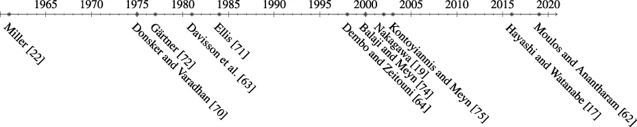
5.2.3 Timeline
5.3 Parameter estimation
Let , and suppose we wish to estimate , from one trajectory X1, …, Xn from a stationary Markov chain with transition matrix and stationary distribution . An important special case is when there exists such that for any , g(x, x′) = f(x′). Then, the quantity of interest is simply . The sample mean evaluated on a stationary Markov trajectory X1, …, Xn is defined by
The statistical behavior of is of particular interest for the topic of Markov Chain Monte Carlo methods. By using the strong law of large numbers, the almost sure convergence to the true expectation holds:Furthermore, defining the asymptotic variance of f asthe following Markov chain version of the central limit theorem [65] holds
Although asymptotic analysis may be of mathematical interest, for modern tasks, it is crucial to have a finite sample theory that explains the behavior of the sample mean. With regard to the original bivariate function problem, the sample mean for a sliding window of pairs of observations can be defined as follows:
One can construct by exponential tilting the following one-dimensional parametric family of transition matrices:where Rθ and ψ are fixed using the PF theory (see Section 3.2). Essentially, is a one-dimensional e-family of transition matrices, and for θ = 0, the original P is recovered. At any natural parameter , the quantity of interest is the expectation parameter η(θ) of Pθ. Recall from (18) that the Fisher information at coordinates θ can be expressed as the second derivative of the potential function, that is, . There exists [15, Lemma 6.2] a constant such that
Defining the asymptotic variance for the bivariate g asit follows that
Note that it coincides with the reciprocal of the Fisher information with respect to the expectation parameter; see Eq. 18. Essentially, this establishes that the sample mean evaluated on pairs of observations is asymptotically efficient; it attains the Markov counterpart of the Cramér–Rao lower bound. Similar results for the multi-parametric case, non-stationary case, and curved exponential families are obtained in [15].
5.4 Hypothesis testing
We let be two irreducible stochastic matrices with respective stationary distributions π0 and π1. We call P0 the null hypothesis and P1 the alternative hypothesis. We observe a trajectory X0, X1, …, Xn sampled from an unknown Markov chain (P0 or P1). A randomized test function is defined by
We interpret as the probability of rejecting the null hypothesis8 under a random experiment [76, p.58]. In particular, if the range of is , the randomized test becomes deterministic. The set of all test functions will be denoted by
We write to denote probability statements and expectations under the null and alternative hypotheses. We define the error probability of the first kind α (also known as the size of the test, type I error, or significance) and second kind β (type II error), respectively, as follows:
Then, 1 −
βis called the power of the test. Fixing
, we define the most powerful test to be the test function
that maximizes the power under the size constraint
:
(i) .
(ii) for any .
The Neyman–Pearson lemma asserts the existence of a test, which can be achieved through the likelihood ratio test.
Lemma 5.1
[
78].
There existandsuch that(i)
(a).
(b)
(ii) Ifsatisfies (a) and (b) for, thenis most powerful at levelα.
If we ignore the effect of the initial distribution that is negligible asymptotically, the Neyman–Pearson accepts the null hypothesis iffor a threshold η and observation (x1, …, xn). Employing the large deviation bound (e.g., [17, Section 8]), we can evaluate the Neyman-Pearson test’s performance in terms of rare events as follows:whereis the exponential family passing through P0 and P1 (see Figure 8), and is the intersection of and the mixture family given by
FIGURE 8

Geometric interpretation of the Neyman–Pearson test as the orthogonal bisector to the e-geodesic passing through both the null and alternative hypotheses.
Note that the e-family and the m-family are orthogonal in that the Pythagorean identity holdsfor any and . The Neyman–Pearson test can be understood as a method that bisects the space by means of an m-family, which is perpendicular to the e-family that links the two hypotheses. For a given 0 < r < D(P0‖P1), if we set the threshold η = η(r) so that D(Pθ(η(r))‖P0) = r, the Neyman–Pearson test attains the exponential trade-off:
In fact, it can be proved that D(Pθ(η(r))‖P1) is the optimal attainable exponent of the type II error probability among any tests such that the type I error probability is less than e−nr. Furthermore, it also holds thatand the optimal exponential trade-off between the type I and type II error probability can be attained by the so-called Hoeffding test. For a more detailed derivation of these results and finite length analysis, see [17, 19].
5.4.1 Historical remarks and timeline
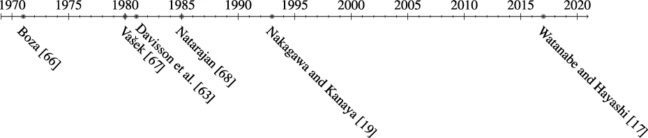
Binary hypothesis testing is one of the well-studied problems in information theory. The use of the Perron–Frobenius theory in this context can be traced back to the 1970s and 1980s [63, 66–68]. The geometrical interpretation of the binary hypothesis testing for Markov chains was first studied in [19]. More recently, the finite length analysis of the binary hypothesis testing for Markov chains was developed in [17] using tools from the information geometry. The binary hypothesis testing is also well studied for quantum systems; for results on quantum systems with memory, see [69].
Statements
Author contributions
GW drafted the initial version, which was subsequently reviewed and edited by both authors. All authors contributed to the article and approved the submitted version.
Funding
GW was supported by the Special Postdoctoral Researcher Program (SPDR) of RIKEN and the Japan Society for the Promotion of Science KAKENHI under Grant 23K13024. SW was supported in part by JSPS KAKENHI under Grant 20H02144.
Acknowledgments
The authors are thankful to the referees for their numerous comments, which helped improve the quality of this manuscript, and for bringing reference [81] to their attention.
Conflict of interest
The authors declare that the research was conducted in the absence of any commercial or financial relationships that could be construed as a potential conflict of interest.
Publisher’s note
All claims expressed in this article are solely those of the authors and do not necessarily represent those of their affiliated organizations or those of the publisher, the editors, and the reviewers. Any product that may be evaluated in this article, or claim that may be made by its manufacturer, is not guaranteed or endorsed by the publisher.
Footnotes
1.^As is customary in the literature, θ denotes both the coordinates of a point in context and the corresponding chart map.
2.^In our definition of m-family, we do not allow a redundant choice of Q0, Q1, …, Qd to express ; if we allow a redundant choice, Ξ need not be an open set and d need not coincide with the dimension of .
3.^The reason for this name will become clear in (21).
4.^When discussing geodesic convexity in this section, we only consider the section of the geodesic joining the two points, achieved for parameter t ∈ [0, 1], not the entire geodesic.
5.^For , itself is an e-family, which is a strict submanifold of .
6.^Note that log U is of the form f(x′) − f(x) + c for some function f and constant c.
7.^The fact that the second derivative of ψ(θ) coincides with the asymptotic variance was clarified in [15].
8.^Note that Nakagawa and Kanaya [19] used a different notation convention, where outputs the probability of accepting the null hypothesis.
References
1.
DiaconisPMicloL. On characterizations of Metropolis type algorithms in continuous time. ALEA: Latin Am J Probab Math Stat (2009) 6:199–238.
2.
ChoiMCHWolferG. Systematic approaches to generate reversiblizations of non-reversible Markov chains (2023). arXiv:2303.03650.
3.
HayashiM. Local equivalence problem in hidden Markov model. Inf Geometry (2019) 2, 1–42. 10.1007/s41884-019-00016-z
4.
HayashiM. Information geometry approach to parameter estimation in hidden Markov model. Bernoulli (2022) 28, 307–42. 10.3150/21-BEJ1344
5.
AmariS-i.NagaokaH. Methods of information geometry, 191. American Mathematical Soc. (2007).
6.
AyNJostJVân LêHSchwachhöferL. Information geometry, 64. Springer (2017).
7.
NagaokaH. The exponential family of Markov chains and its information geometry. In: The proceedings of the symposium on information theory and its applications, 28-2 (2005). p. 601–604.
8.
VidyasagarM. An elementary derivation of the large deviation rate function for finite state Markov chains. Asian J Control (2014) 16:1–19. 10.1002/asjc.806
9.
LevinDAPeresYWilmerEL. Markov chains and mixing times. second edition. American Mathematical Soc. (2009).
10.
RachedZAlajajiFCampbellLL. The Kullback-Leibler divergence rate between Markov sources. IEEE Trans Inf Theor (2004) 50:917–21. 10.1109/TIT.2004.826687
11.
EguchiS. Second order efficiency of minimum contrast estimators in a curved exponential family. Ann Stat (1983) 11:793–803. 10.1214/aos/1176346246
12.
EguchiS. A differential geometric approach to statistical inference on the basis of contrast functionals. Hiroshima Math J (1985) 15:341–91. 10.32917/hmj/1206130775
13.
WolferGWatanabeS. Information geometry of reversible Markov chains. Inf Geometry (2021) 4:393–433. 10.1007/s41884-021-00061-7
14.
ItoHAmariS. Geometry of information sources. In: Proceedings of the 11th symposium on information theory and its applications. SITA ’88 (1988). p. 57–60.
15.
HayashiMWatanabeS. Information geometry approach to parameter estimation in Markov chains. Ann Stat (2016) 44:1495–535. 10.1214/15-AOS1420
16.
BregmanLM. The relaxation method of finding the common point of convex sets and its application to the solution of problems in convex programming. USSR Comput Math Math Phys (1967) 7:200–17. 10.1016/0041-5553(67)90040-7
17.
WatanabeSHayashiM. Finite-length analysis on tail probability for Markov chain and application to simple hypothesis testing. Ann Appl Probab (2017) 27:811–45. 10.1214/16-AAP1216
18.
MatumotoTAny statistical manifold has a contrast function—On the C3-functions taking the minimum at the diagonal of the product manifold. Hiroshima Math J (1993) 23:327–32. 10.32917/hmj/1206128255
19.
NakagawaKKanayaF. On the converse theorem in statistical hypothesis testing for Markov chains. IEEE Trans Inf Theor (1993) 39:629–33. 10.1109/18.212294
20.
AdamčíkM. The information geometry of Bregman divergences and some applications in multi-expert reasoning. Entropy (2014) 16:6338–81. 10.3390/e16126338
21.
WolferGWatanabeS. Geometric aspects of data-processing of Markov chains (2022). arXiv:2203.04575.
22.
MillerH. A convexity property in the theory of random variables defined on a finite Markov chain. Ann Math Stat (1961) 32:1260–70. 10.1214/aoms/1177704865
23.
CsiszárICoverTChoiB-S. Conditional limit theorems under Markov conditioning. IEEE Trans Inf Theor (1987) 33:788–801. 10.1109/TIT.1987.1057385
24.
TakeuchiJ-i.BarronAR. Asymptotically minimax regret by Bayes mixtures. In: Proceedings 1998 IEEE International Symposium on Information Theory (Cat No 98CH36252). IEEE (1998). p. 318.
25.
TakeuchiJKawabataT. Exponential curvature of Markov models. In: Proceedings. 2007 IEEE International Symposium on Information Theory; June 2007; Nice, France. IEEE (2007). p. 2891–5.
26.
TakeuchiJNagaokaH. On asymptotic exponential family of Markov sources and exponential family of Markov kernels (2017). [Dataset].
27.
FeiginPDConditional exponential families and a representation theorem for asympotic inference. Ann Stat (1981) 9:597–603. 10.1214/aos/1176345463
28.
KüchlerUSørensenM. On exponential families of Markov processes. J Stat Plann inference (1998) 66:3–19. 10.1016/S0378-3758(97)00072-4
29.
HudsonIL. Large sample inference for Markovian exponential families with application to branching processes with immigration. Aust J Stat (1982) 24:98–112. 10.1111/j.1467-842X.1982.tb00811.x
30.
StefanovVT. Explicit limit results for minimal sufficient statistics and maximum likelihood estimators in some Markov processes: Exponential families approach. Ann Stat (1995) 23:1073–101. 10.1214/aos/1176324699
31.
KüchlerUSørensenM. Exponential families of stochastic processes: A unifying semimartingale approach. Int Stat Review/Revue Internationale de Statistique (1989) 57:123–44. 10.2307/1403382
32.
SørensenM. On sequential maximum likelihood estimation for exponential families of stochastic processes. Int Stat Review/Revue Internationale de Statistique (1986) 54:191–210. 10.2307/1403144
33.
KellyFP. Reversibility and stochastic networks. Cambridge University Press (2011).
34.
BrooksSGelmanAJonesGMengX-L. Handbook of Markov chain Monte Carlo. Chapman & Hall/CRC Press (2011).
35.
SchrödingerE. Über die umkehrung der naturgesetze. Sitzungsberichte der preussischen Akademie der Wissenschaften, physikalische mathematische Klasse (1931) 8:144–53.
36.
KolmogorovA. Zur theorie der Markoffschen ketten. Mathematische Annalen (1936) 112:155–60. 10.1007/BF01565412
37.
KolmogorovA. Zur umkehrbarkeit der statistischen naturgesetze. Mathematische Annalen (1937) 113:766–72. 10.1007/BF01571664
38.
DobrushinRLSukhovYMFritzJ. A.N. Kolmogorov - the founder of the theory of reversible Markov processes. Russ Math Surv (1988) 43:157–82. 10.1070/RM1988v043n06ABEH001985
39.
HsuDKontorovichALevinDAPeresYSzepesváriCWolferG. Mixing time estimation in reversible Markov chains from a single sample path. Ann Appl Probab (2019) 29:2439–80. 10.1214/18-AAP1457
40.
PistoneGRogantinMP. The algebra of reversible Markov chains. Ann Inst Stat Math (2013) 65:269–93. 10.1007/s10463-012-0368-7
41.
DiaconisPRollesSW. Bayesian analysis for reversible Markov chains. Ann Stat (2006) 34:1270–92. 10.1214/009053606000000290
42.
KönigD. Theorie der endlichen und unendlichen Graphen: Kombinatorische Topologie der Streckenkomplexe, 16. Akademische Verlagsgesellschaft mbh (1936).
43.
BirkhoffG. Three observations on linear algebra. Univ Nac Tacuman, Rev Ser A (1946) 5:147–51.
44.
Von NeumannJ. A certain zero-sum two-person game equivalent to the optimal assignment problem. Contrib Theor Games (1953) 2:5–12. 10.1515/9781400881970-002
45.
ČencovNN. Statistical decision rules and optimal inference, Transl. Math. Monographs, 53. Providence-RI: Amer. Math. Soc. (1981).
46.
CampbellLL. An extended Čencov characterization of the information metric. Proc Am Math Soc (1986) 98:135–41. 10.1090/S0002-9939-1986-0848890-5
47.
LêHV. The uniqueness of the Fisher metric as information metric. Ann Inst Stat Math (2017) 69:879–96. 10.1007/s10463-016-0562-0
48.
BurkeCRosenblattM. A Markovian function of a Markov chain. Ann Math Stat (1958) 29:1112–22. 10.1214/aoms/1177706444
49.
RogersLCPitmanJ. Markov functions. Ann Probab (1981) 9:573–82. 10.1214/aop/1176994363
50.
KemenyJGSnellJLMarkov chains, 6. New York: Springer-Verlag (1976).
51.
LebanonG. An extended Čencov-Campbell characterization of conditional information geometry. In: Proceedings of the 20th conference on Uncertainty in artificial intelligence; July 2004 (2004). p. 341–8.
52.
LebanonG. Axiomatic geometry of conditional models. IEEE Trans Inf Theor (2005) 51:1283–94. 10.1109/TIT.2005.844060
53.
MontúfarGRauhJAyN. On the Fisher metric of conditional probability polytopes. Entropy (2014) 16:3207–33. 10.3390/e16063207
54.
WolferGWatanabeS. A geometric reduction approach for identity testing of reversible Markov chains. In: Geometric Science of Information (to appear): 6th International Conference, GSI 2023; August–September, 2023; Saint-Malo, France. Springer (2023). Proceedings 6.
55.
WeinbergerMJRissanenJFederM. A universal finite memory source. IEEE Trans Inf Theor (1995) 41:643–52. 10.1109/18.382011
56.
WillemsFShtar’kovYTjalkensT. The context tree weighting method: Basic properties. IEEE Trans Inf Theor (1995) 41:653–64. 10.1109/18.382012
57.
TakeuchiJNagaokaH. Information geometry of the family of Markov kernels defined by a context tree. In: 2017 IEEE Information Theory Workshop (ITW). IEEE (2017). p. 429–33.
58.
SpitzerF. A variational characterization of finite Markov chains. Ann Math Stat (1972) 43:303–7. 10.1214/aoms/1177692723
59.
JustesenJHoholdtT. Maxentropic Markov chains (corresp). IEEE Trans Inf Theor (1984) 30:665–7. 10.1109/TIT.1984.1056939
60.
DudaJ. Optimal encoding on discrete lattice with translational invariant constrains using statistical algorithms (2007). arXiv preprint arXiv:0710.3861.
61.
BurdaZDudaJLuckJ-MWaclawB. Localization of the maximal entropy random walk. Phys Rev Lett (2009) 102:160602. 10.1103/PhysRevLett.102.160602
62.
MoulosVAnantharamV. Optimal chernoff and hoeffding bounds for finite state Markov chains (2019). arXiv preprint arXiv:1907.04467.
63.
DavissonLLongoGSgarroA. The error exponent for the noiseless encoding of finite ergodic Markov sources. IEEE Trans Inf Theor (1981) 27:431–8. 10.1109/TIT.1981.1056377
64.
DemboAZeitouniO. Large deviations techniques and applications. Springer (1998).
65.
JonesGL. On the Markov chain central limit theorem. Probab Surv (2004) 1:299–320. 10.1214/154957804100000051
66.
BozaLB. Asymptotically optimal tests for finite Markov chains. Ann Math Stat (1971) 42:1992–2007. 10.1214/aoms/1177693067
67.
VašekK. On the error exponent for ergodic Markov source. Kybernetika (1980) 16:318–29. 10.1109/TIT.1981.1056377
68.
NatarajanS. Large deviations, hypotheses testing, and source coding for finite Markov chains. IEEE Trans Inf Theor (1985) 31:360–5. 10.1109/TIT.1985.1057036
69.
MosonyiMOgawaT. Two approaches to obtain the strong converse exponent of quantum hypothesis testing for general sequences of quantum states. IEEE Trans Inf Theor (2015) 61:6975–94. 10.1109/TIT.2015.2489259
70.
DonskerMDVaradhanSS. Asymptotic evaluation of certain Markov process expectations for large time, i. Commun Pure Appl Math (1975) 28:1–47. 10.1109/TIT.2015.2489259
71.
EllisRS. Large deviations for a general class of random vectors. Ann Probab (1984) 12:1–12. 10.1214/aop/1176993370
72.
GärtnerJ. On large deviations from the invariant measure. Theor Probab Its Appl (1977) 22:24–39. 10.1137/1122003
73.
GrayRM. Entropy and information theory. Springer Science & Business Media (2011).
74.
BalajiSMeynSP. Multiplicative ergodicity and large deviations for an irreducible Markov chain. Stochastic Process their Appl (2000) 90:123–44. 10.1016/S0304-4149(00)00032-6
75.
KontoyiannisIMeynSP. Spectral theory and limit theorems for geometrically ergodic Markov processes. Ann Appl Probab (2003) 13:304–62. 10.1214/aoap/1042765670
76.
LehmannELRomanoJPCasellaGTesting statistical hypotheses, 3. Springer (2005).
77.
NakagawaK. The geometry of m/d/1 queues and large deviation. Int Trans Oper Res (2002) 9:213–22. 10.1111/1475-3995.00351
78.
NeymanJPearsonES. Ix. on the problem of the most efficient tests of statistical hypotheses. Philosophical Trans R Soc Lond Ser A, Containing Pap a Math or Phys Character (1933) 231:289–337. 10.1098/rsta.1933.0009
79.
NielsenF. An elementary introduction to information geometry. Entropy (2020) 22:1100. 10.3390/e22101100
80.
ČencovNN. Algebraic foundation of mathematical statistics. Ser Stat (1978) 9:267–76. 10.1080/02331887808801428
81.
GaspardP. Time-reversed dynamical entropy and irreversibility in Markovian random processes. J Stat Phys (2004) 117:599–615. 10.1007/s10955-004-3455-1
Summary
Keywords
Markov chains (60J10), data processing, information geometry, congruent embeddings, Markov morphisms
Citation
Wolfer G and Watanabe S (2023) Information geometry of Markov Kernels: a survey. Front. Phys. 11:1195562. doi: 10.3389/fphy.2023.1195562
Received
28 March 2023
Accepted
08 June 2023
Published
27 July 2023
Volume
11 - 2023
Edited by
Jun Suzuki, The University of Electro-Communications, Japan
Reviewed by
Antonio Maria Scarfone, National Research Council (CNR), Italy
Marco Favretti, University of Padua, Italy
Fabio Di Cosmo, Universidad Carlos III de Madrid de Madrid, Spain
Updates
Copyright
© 2023 Wolfer and Watanabe.
This is an open-access article distributed under the terms of the Creative Commons Attribution License (CC BY). The use, distribution or reproduction in other forums is permitted, provided the original author(s) and the copyright owner(s) are credited and that the original publication in this journal is cited, in accordance with accepted academic practice. No use, distribution or reproduction is permitted which does not comply with these terms.
*Correspondence: Geoffrey Wolfer, geoffrey.wolfer@riken.jp
Disclaimer
All claims expressed in this article are solely those of the authors and do not necessarily represent those of their affiliated organizations, or those of the publisher, the editors and the reviewers. Any product that may be evaluated in this article or claim that may be made by its manufacturer is not guaranteed or endorsed by the publisher.