Numerical approximations for fluid flow and heat transfer in the boundary layer with radiation through multiple Lie similarity transformations

1 Introduction

Heat transfer in thin films has garnered significant attention in various manufacturing processes. For example, the process of cooling thin films during the extrusion of polymer sheets, metal sheets, wire coatings, painting, polishing, and many other processes involves heat transfer in thin liquid films. Moreover, some industrial processes, such as surface paint and heat treatments on ceramics, involve radiation treatment to control the temperature of the fluid and boundary layer thickness without affecting the temperature of the surface. In many of these applications, the final product requires a smooth surface finish, which is attained by controlling the rate of heat transfer in these films. With advancements in manufacturing techniques and processes, more accurate methods are required to predict the physics of heat transfer in these types of fluid flows. In some industries, radiation treatments are performed to control the temperature, unsteadiness, and rate of heat transfer in the fluid by altering the surface temperature, such as surface paints on metal sheets in the automobile industry, surface polishing on ceramic products, and thin-walled solar water heaters. These applications require applying thermal radiation effects in energy equations while modeling fundamental boundary layer flows.

Crane [1] investigated the fluid flow driven on a semi-infinite linearly stretching surface, which Wang [2] extended to include the unsteady effects of hydrodynamics in thin-film stretching sheets. Andersson et al. [3] modeled the non-Newtonian fluid flow in a thin film on an unsteady stretching sheet using a power law. Andersson et al. [4] studied this phenomenon further by incorporating heat transfer. Moreover, on an unsteady stretching surface, Chen [5] studied non-Newtonian fluid flow; Dandapat et al. [6] included thermocapillary effects; Chen [7] illustrated viscous dissipation effects on heat transfer in a thin-film flow of a non-Newtonian fluid; Wang [8] obtained analytical solutions for the problem considered in [4] using the homotopy analysis method (HAM); and Dandapat et al. [9] explored the heat transfer in thin films with variable thermal conductivity, viscosity, and thermocapillarity. Several other authors [10–15] developed numerical and analytical solutions to similar problems with additional physical conditions and constraints. Liu and Megahed [16] illustrated the effects of thermal radiation, variable thermal conductivity, and viscosity on heat transfer and fluid flow in a thin film on an unsteady stretching sheet. Furthermore, Kumar [17] scrutinized the 3D flow and non-linear radiative heat transfer of non-Newtonian nanoparticles over an exponentially stretching sheet. Kumar [18] analyzed the flow and heat transfer of non-Newtonian nanofluid over a stretching sheet by considering the slip factor. Reddy et al. [19] demonstrated the transverse magnetic flow over a Reiner–Philippoff nanofluid by considering solar radiation. Kumar [20] studied the ferromagnetic hybrid nanofluid effects on heat transfer under solar radiation. Azam et al. [21] examined the transient bioconvection and activation energy impacts on Casson nanofluid with gyrotactic microorganisms and non-linear radiation. Puneeth et al. [22] considered a 3D flow of a nanofluid with non-linear thermal radiation and multi-slip conditions. Sudharani et al. [23] analyzed the influence of slip flow and linear radiation on a hybrid and tri-hybrid nanofluid. Naik et al. [24] investigated heat transfer under the influence of magnetic dipole. In all these studies, the similarity transformations remained the same. In such boundary layer problems, the flow originates from the origin, and the stretching of the elastic sheet causes it to flow in a plane parallel to its motion. Restriction of the stretching sheet velocity and temperature, namely, when $U\left(x,t\right)$ and $T\left(x,t\right)$ depend on the $x-$ distance from the origin and time, enables the mapping of systems of boundary layer partial differential equations (PDEs) into systems of ordinary differential equations (ODEs) [2]. The systems of equations thus obtained are non-linear and coupled; therefore, analytic and approximate solution schemes are employed to construct the velocity and temperature profiles.

In this study, we used the Lie symmetry method [25–27] to derive similarity transformations. Safdar et al. [28] proposed Lie similarity transformations for an unsteady flow in a thin film over a stretching sheet and constructed analytic solutions using Lie point symmetries. In their work, instead of using $U\left(x,t\right)=bx/\left(1-at\right)$ to obtain the fluid velocity, the invariance of the obtained Lie symmetry algebra was used to derive a general form for $U\left(x,t\right)$ along with the stretching sheet temperature $T_s\left(x,t\right)$ and film thickness $h\left(t\right)$. Bilal et al. [29] recently proposed a method to obtain the Lie similarity transformations for heat transfer in boundary layer flow with additional parameters. For a system of differential equations (DEs), the Lie point symmetry offers reduction based on functions that remain invariant under the action of these generators. For a PDE system, these invariants reduce the number of dependent and independent terms. Such consecutive reductions in the independent variables of the flow PDEs resulted in a system of ODEs. In this study, we found seven Lie point symmetry generators for a system of PDEs describing the boundary layer flow and heat transfer in a thin film on an unsteady stretching surface in the presence of radiation, with three dependent and three independent terms. In the next step, we reduced one independent variable of the system by applying invariants associated with the linear combinations of the obtained symmetries. Consequently, we let the reduction procedure dictate the form of the velocity components using specific boundary conditions. Another reduction was achieved through the invariants of the symmetries of the once-reduced system. This double reduction revealed a system of ODEs corresponding to the flow and heat transfer PDEs. Similarity transformations were attained using the invariants derived in both cases. This directly mapped the flow and heat transfer equations to the same systems of ODEs obtained through separate reductions. We showed that five similarity transformations exist for flow and heat transfer equations. These transformations corresponded only to linear combinations of the Lie point symmetries for which both the velocity and temperature of the stretching sheet were retained as functions of space $x$ and time $t$. These new similarity transformations revealed more than one type of ODE system. Hence, the Lie symmetry procedure led to more than one class of system of equations for studying the flow and heat transfer. We used finite-difference approximations to draw the velocity and temperature profiles for the systems of the ODEs extracted from the flow model via similarity transformations.

Previous studies on flow and heat transfer have primarily focused on the solution method(s) or analysis with additional parameters by utilizing the pre-existing basic similarity transformations given by [2,8]. Single reductions of systems of differential equations representing steady flows are performed using such similarity transformations, whereas double reductions through these transformations are performed for unsteady fluid flows. In these transformations, the velocity of the elastic sheet is considered $U\left(x,t\right)=bx/\left(1-at\right)$, which later directly ensures the fluid velocity $u$-velocity is a component in these transformations, such that $u=bx{f}^{\prime }\left(\eta \right)/\left(1-at\right)$. This is problematic when a real-world problem is modeled using velocity and temperature as inputs, where the velocity of the flow exceeds that of the stretching sheet (most real-world flows).

Bilal et al. [30] recently conducted a detailed heat transfer analysis of boundary layer flow in the presence of radiation using two different types of transformations. It was observed that the valid transformation obtained using Lie point symmetries yields results in the different regions compared with the existing transformations. The comparison showed that the previously existing transformation is valid only for steady and marginally accelerating fluid (unsteadiness). However, the Lie transformations provide a valid solution for any range of unsteadiness in the fluid. In addition, the previous transformations are valid for a specific time interval, which depends on a range of unsteadiness parameters. However, the Lie similarity transformations provide valid solutions at any given time. This motivates the author to derive all the Lie point similarity transformations associated with the system of PDEs representing the flow and heat transfer in the boundary layer in the presence of radiation.

The remainder of this study is organized as follows: Section 2 describes the mathematical formulation and Lie point symmetry transformations/generators of the flow. The numerical solutions are presented in Section 3. The results and discussion based on the velocity and temperature profiles are presented in Section 4, and conclusions are presented in Section 5.

2 Mathematical formulation and construction of similarity transformations

Consider a fully developed, viscous, nonvolatile, unsteady, incompressible, two-dimensional fluid flowing on a thin horizontal elastic surface and emerging from a hole (shown in Figure 1) that emerges from the origin of the $\left(x,y\right)$ coordinate system. The fluid viscosity was unaffected by temperature changes, and the buoyancy effects were negligible. The velocity and temperature changed with time $t$ and $x$-coordinate, and the streamwise diffusion terms were neglected. The smoothness of the thin film surface was assumed to be free of any type of wave. Considering all these assumptions, we obtained the following boundary layer equations:

$\begin{array}{c}{\mathrm{u}}_x+{\mathrm{v}}_y=0,\hfill \\ {{\mathrm{u}}_t+\mathrm{u}\mathrm{u}}_x+{\mathrm{v}\mathrm{u}}_y-\frac{\mathrm{\mu }}{\rho }{\mathrm{u}}_{yy}=0,\hfill \\ {T_t+\mathrm{u}\mathrm{T}}_x+{\mathrm{v}\mathrm{T}}_y-\frac{\kappa }{\rho C_p}{T}_{yy}-\frac{1}{\rho C_p}{\mathrm{q}}_y^r=0,\hfill \end{array}(1)$

such that

$\mathrm{y}=0:\mathrm{u}=\mathrm{U}\left(\mathrm{x},\mathrm{t}\right),\mathrm{v}=0,\mathrm{T}={\mathrm{T}}_s\left(\mathrm{x},\mathrm{t}\right),\mathrm{y}=\mathrm{h}\left(\mathrm{t}\right):{\mathrm{u}}_y={\mathrm{T}}_y=0,\mathrm{v}={\mathrm{h}}_t\left(\mathrm{t}\right).(2)$

FIGURE 1

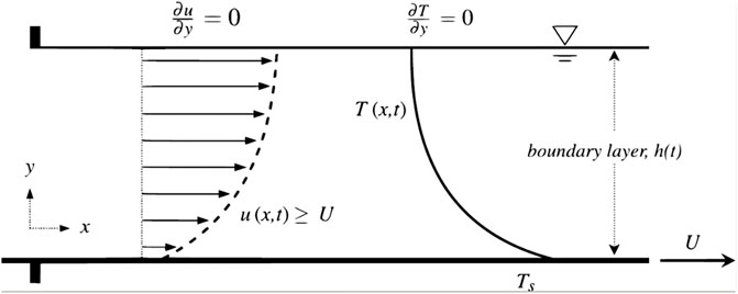
FIGURE 1. Fluid flow and heat transfer in the boundary layer.

In the aforementioned equations, the $u$- and $v$-velocities are in the $x$- and $y$-directions, respectively. $T$ and $t$ denote the temperature and time, respectively. $\mu$ is the dynamic viscosity; $\rho$ is the density of the fluid; $C_p$ is the specific heat of fluid at constant pressure; $\kappa$ is the thermal conductivity; $q^r$ is the heat flux under the radiation, and $h\left(t\right)$ is the boundary layer film thickness. The subscripts in (Eqs 1, 2) represent partial derivatives; for example, $v_y$ denotes the $y$ derivative of the $v$-velocity. The velocity of the stretching surface in $x$-direction is denoted by $U\left(x,t\right)$. Wang [2] provided the following form of the stretching velocity $U\left(x,t\right)$ by restricting the motion to

$U\left(x,t\right)=\frac{bx}{1-at},(3)$

According to [4], the surface temperature $T_s\left(x,t\right)$ is expressed as

$T_s\left(x,t\right)=T_0-T_{ref}\left(\frac{d\rho x^2}{2\mu }\right){\left(1-at\right)}^{-\frac{3}{2}}.(4)$

According to the Rosseland approximation [31], $q_r$ is

$q^r=-\frac{4\sigma }{3k_a}{T}_y^4.(5)$

In Eqs 3, 4, $a,b,$ and $d$ are constants; the first two possess the dimensions of $tim{e}^{-1}$, whereas the third is a constant of proportionality. Moreover, $T_0$ and $T_{ref}$ denote the ambient and reference temperatures, respectively. In Eq. 5, $k_a$ and $\sigma$ represent the mean absorption coefficient and Stefan–Boltzmann constant, respectively. Raptis [32] expressed the temperature as a linear function for small variations in it. By expanding $T^4$ about $T_0$ with diminishing higher order terms of the Taylor series, we obtain

$T^4\cong 4T{T}_0^3-3T_0^4.(6)$

The formulas of $U\left(x,t\right)-$ surface velocity (Eq. 3) and $T_s\left(x,t\right)-$ temperature (Eq. 4) lead to the following similarity transformations:

$\begin{array}{c}\eta =\frac{1}{\sqrt{\frac{\rho b}{\left(1-at\right)\mu }}}\frac{y}{\beta },u=\frac{bx}{1-at}{f}^{\prime }\left(\eta \right),v=\beta \sqrt{-\frac{b\mu }{\rho \left(1-at\right)}}f\left(\eta \right),\hfill \\ T=T_0-T_{ref}\left(\frac{d\rho x^2}{2\mu }\right){\left(1-at\right)}^{-\frac{3}{2}}\vartheta \left(\eta \right),\hfill \end{array}(7)$

where $\eta$ and $\vartheta$ represent the stream function, similarity variable, and dimensionless temperature, respectively, whereas $\beta$ denotes the unknown dimensionless film thickness. Substituting the similarity transformations Eq. 7 into Eq. 1, the transformed system can be written as

$\begin{array}{c}{f}^{‴}+\lambda \left(f{f}^{″}-{f^{\prime }}^2-S{f}^{\prime }-\frac{S\eta f^{″}}{2}\right)=0,\hfill \\ \frac{{\vartheta }^{″}}{\mathit{Pr}}\left(1+R\right)+\lambda \left(f{\vartheta }^{\prime }-2f^{\prime }\vartheta -\frac{S\eta {\vartheta }^{\prime }}{2}-\frac{3S\vartheta }{2}\right)=0.\hfill \end{array}(8)$

Likewise, the boundary conditions (Eq. 2) are transformed to

$\begin{array}{c}\eta =0:f\left(\eta \right)=0,\vartheta \left(\eta \right)=f^{\prime }\left(\eta \right)=1,\hfill \\ \eta =1:f\left(\eta \right)=\frac{S}{2},{\vartheta }^{\prime \left(\eta \right)}=f^{″}\left(\eta \right)=0,\hfill \end{array}(9)$

where

$R=\frac{16\sigma T_0^3}{3k_a\kappa }.(10)$

The aforementioned approach serves as a reference procedure for converting a system of PDEs into a system of ODEs. The transformed system (8) is valid only when $t<a^{-1}$. In Eqs (8) and (9), the prime ($\prime$) indicates a derivative with respect to the similarity variable $\eta$; the dimensionless film thickness is denoted by $\lambda ={\beta }^2$; $\mathit{Pr}=\mu \frac{C_p}{\kappa }$ is the Prandtl number; $R$ denotes the radiation parameter; and $S=a/b$ is the dimensionless unsteadiness parameter.

2.1 Lie symmetries and symmetry transformations

Lie developed an algebraic approach for constructing Lie point symmetries associated with differential equations [25–27]. These point transformations map the dependent and independent variables of a differential equation into new dependent and independent variables. These mappings leave the differential equations form-invariant such that their properties (e.g., linearity/non-linearity, order, and type) remain unaltered. Here, for the system of PDEs considered (1), we followed the procedure described by [28] for such systems and their associated conditions (2). The Lie point symmetry associated with system (1) in the general form can be written as

$\mathbf{X}={\xi }_1\frac{\partial }{\partial x}+{\xi }_2\frac{\partial }{\partial t}+{\xi }_3\frac{\partial }{\partial y}+{\varphi }_1\frac{\partial }{\partial T}+{\varphi }_2\frac{\partial }{\partial u}+{\varphi }_3\frac{\partial }{\partial v},(11)$

where ${\xi }_i$, ${\varphi }_i$, for $i=\mathrm{1,2,3},$ are known as infinitesimal coordinates that are functions $\left(x,t,y\right)$. System (1) and related conditions (2) possess partial derivatives up to order two; hence, ${\mathbf{X}}^{\left[1\right]}-$ first extension and ${\mathbf{X}}^{\left[2\right]}-$ second extension of the generator (11) are required to establish the invariance of (1) and (2) under (11). These extensions can be obtained from

${\mathbf{X}}^{\left[2\right]}=\mathbf{X}+{\varphi }_k^t\frac{\partial }{\partial {\zeta }_{k,t}}+{\varphi }_k^x\frac{\partial }{\partial {\zeta }_{k,x}}+{\varphi }_k^y\frac{\partial }{\partial {\zeta }_{k,y}}+{\varphi }_k^{tt}\frac{\partial }{\partial {\zeta }_{k,tt}}+{\varphi }_k^{xx}\frac{\partial }{\partial {\zeta }_{k,xx}}+{\varphi }_k^{yy}\frac{\partial }{\partial {\zeta }_{k,yy}}.(12)$

The coefficients in these extensions are obtained from

${\varphi }_k^n=D_n{\varphi }_k-{\zeta }_{k,t}{D}_n\left({\xi }_1\right)-{\zeta }_{k,x}{D}_n\left({\xi }_2\right)-{\zeta }_{k,y}{D}_n\left({\xi }_3\right),(13)$

where $n\in \left\{t,x,y\right\}$ and $k=\mathrm{1,2,3}$. The second extension coefficients are derived using

$\begin{array}{c}{\varphi }_k^{tt}=D_t{\varphi }_k^t-{\zeta }_{k,tt}{D}_n\left({\xi }_1\right)-{\zeta }_{k,tx}{D}_n\left({\xi }_2\right)-{\zeta }_{k,ty}{D}_n\left({\xi }_3\right),\\ {\varphi }_k^{xx}=D_x{\varphi }_k^x-{\zeta }_{k,tx}{D}_n\left({\xi }_1\right)-{\zeta }_{k,xx}{D}_n\left({\xi }_2\right)-{\zeta }_{k,xy}{D}_n\left({\xi }_3\right),\\ {\varphi }_k^{yy}=D_y{\varphi }_k^y-{\zeta }_{k,ty}{D}_n\left({\xi }_1\right)-{\zeta }_{k,xy}{D}_n\left({\xi }_2\right)-{\zeta }_{k,yy}{D}_n\left({\xi }_3\right).\end{array}(14)$

The subscript in $D_t$ is a total derivative with respect to $t$, which expands as

$D_n=\frac{\partial }{\partial n}+{\zeta }_{k,n}\frac{\partial }{\partial k}+{\zeta }_{k,nn}\frac{\partial }{\partial k,n}+\dots ,(15)$

where $n\in \left\{t,x,y\right\}$ and $k=\mathrm{1,2,3}$. To determine the infinitesimal coordinates ${\xi }_k$ and ${\varphi }_k$ of operator (11), its second-order extension ${\mathbf{X}}^{\left[2\right]}$ is applied to the system of PDEs (1). For instance, its application to the continuity equation in (1) requires the following invariance criterion:

${\left.{\mathbf{X}}^{\left[\mathbf{2}\right]}\left(\frac{\partial u}{\partial x}+\frac{\partial v}{\partial y}\right)\right|}_{\frac{\partial u}{\partial x}+\frac{\partial v}{\partial y}=0}=0.(16)$

This criterion is evaluated using the continuity equation of system (1). The partial derivatives and coefficients of $u,v$, and $T$ in the resulting equation are zero. Solving these systems simultaneously yields the system of PDEs, which contains ${\xi }_k$ and ${\varphi }_k$ and their partial derivatives. By solving these systems of PDEs, we obtain

$\begin{array}{c}{\xi }_1={\delta }_{6}t+{\delta }_1,{\xi }_2={\delta }_{4}x+{\delta }_{5}t+{\delta }_2,{\xi }_3=\frac{{\delta }_{6}y}{2},\hfill \\ {\varphi }_1=\left({\delta }_4-{\delta }_6\right)u+{\delta }_5,{\varphi }_2=-\frac{{\delta }_{6}v}{2},{\varphi }_3={\delta }_{3}T+{\delta }_7,\hfill \end{array}(17)$

where ${\delta }_1,{\delta }_2,\dots ,{\delta }_7$ are constants that yield the seven Lie point symmetry generators given in Table 1.

TABLE 1

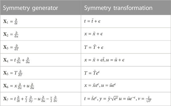
TABLE 1. Lie symmetries and transformations.

MAPLE offers a built-in code, “Infinitesimals,” for computing Lie point symmetries in its package “PDEtools.” We use the same method to obtain the symmetry transformations for system (1), which form a Lie algebra. These symmetry generators ${\mathbf{X}}_1,\dots ,{\mathbf{X}}_7$ and their linear combinations leave system (1) form-invariant.

To obtain similarity transformations using symmetry generators, condition (2) must remain form-invariant when operated by generators. Both velocity and temperature are functions of the time $t$ and $x$-coordinate. However, when we use a single symmetry ${\mathbf{X}}_1,\dots ,{\mathbf{X}}_7$, (considering one at a time), both the velocity $U\left(x,t\right)$ and temperature $T_s\left(x,t\right)$ in (2) become functions of only the time $t$ or $x$-coordinate. However, both must remain functions of the time $t$ and $x$-coordinate. Therefore, $U\left(x,t\right)$ and $T_s\left(x,t\right)$ in (2) become the desired functions when linear combinations of ${\mathbf{X}}_1,\dots ,{\mathbf{X}}_7$ are used considering two at a time. In the present study, five valid combinations in which both boundary conditions with $U\left(x,t\right)$ and $T_s\left(x,t\right)$ became functions of the time $t$ and $x$-coordinate, were obtained.

2.2 Double reductions with similarity transformations

In this subsection, successive double reductions of DEs were used to construct similarity transformations using Lie point symmetry generators. We allowed the symmetry procedure to determine the form of the surface velocity using boundary condition (2). We demonstrate the process of reduction considering the symmetries ${\mathit{X}}_{\mathbf{4}}+{\mathit{X}}_{\mathbf{5}}$. All conditions (2) are left form-invariant by the symmetry combination ${\mathbf{X}}_{\mathbf{4}}+{\mathbf{X}}_{\mathbf{5}}$, with a few exceptions, namely, $\mathit{h}\left(\mathit{t}\right)$, $\mathit{U}\left(\mathit{x},\mathit{t}\right),$ and ${\mathit{T}}_{\mathit{s}}\left(\mathit{x},\mathit{t}\right)$, which are put in place by the considered linear combination. After substituting these boundary conditions, the invariance criterion is as follows:

$\begin{array}{c}{\left.{\left[\mathbf{X}\right.}_{\mathbf{4}}+{\mathbf{X}}_{\mathbf{5}}]\left(u-U\left(x,t\right)\right)\right|}_{u=U\left(x,t\right)}=0,\hfill \\ {\left.{\left[\mathbf{X}\right.}_{\mathbf{4}}+{\mathbf{X}}_{\mathbf{5}}]\left(T-T_s\left(x,t\right)\right)\right|}_{T=T_s\left(x,t\right)}=0.\hfill \end{array}(18)$

By substituting generators and expanding them at $\mathit{u}=\mathit{U}\left(\mathit{x},\mathit{t}\right)$ and $\mathit{T}={\mathit{T}}_{\mathit{s}}\left(\mathit{x},\mathit{t}\right)$, we obtain the following linear PDEs:

$x\frac{\partial U}{\partial x}-u=0,x\frac{\partial T_s}{\partial x}-T+T_0=0.(19)$

Solving the aforementioned linear PDEs, we obtain

$u=x\overline{U}\left(t\right),T=T_0+x{\overline{T}}_s\left(t\right).(20)$

To derive invariants, we apply ${\mathbf{X}}_{\mathbf{4}}+{\mathbf{X}}_{\mathbf{5}}$, on $\mathit{J}\left(\mathit{x},\mathit{t},\mathit{y},\mathit{T},\mathit{u},\mathit{v}\right)$, which results in a PDE:

$t{J}_x+J_u+T{J}_T=0,(21)$

whose solution provides the invariants $\left\{t,y,\frac{u}{x},v,\frac{T}{x}\right\}$. These are assigned as the new independent variables:

$c_1=t,c_2=y,(22)$

and new dependent variables:

$P=\frac{u}{x},Q=v,R=\frac{T}{x}.(23)$

System (1) in these new variables is transformed into

$\begin{array}{c}\mathrm{P}+\frac{\partial \mathrm{Q}}{\partial c_2}=0,\hfill \\ \frac{\partial \mathrm{P}}{\partial c_1}+{\mathrm{P}}^2+\mathrm{Q}\frac{\partial \mathrm{P}}{\partial c_2}=\frac{\mathrm{\mu }}{\rho }\left(\frac{{\partial }^{2}P}{\partial c_2^2}\right),\hfill \\ \frac{\partial \mathrm{R}}{\partial c_1}+\mathrm{PR}+\mathrm{Q}\frac{\partial \mathrm{R}}{\partial c_2}=\frac{\kappa }{\rho C_p}\left(\frac{{\partial }^{2}R}{\partial c_2^2}+\frac{16\sigma T_0^3}{3k_a\kappa }\right),\hfill \end{array}(24)$

whereas the boundary conditions (2) become

${\mathrm{c}}_2=0:\mathrm{P}=\mathrm{F}\left({\mathrm{c}}_1\right),\mathrm{Q}=0,\mathrm{R}=\mathrm{G}\left({\mathrm{c}}_1\right),{\mathrm{c}}_2=\mathrm{h}\left({\mathrm{c}}_1\right):\mathrm{Q}=\frac{\mathrm{d}\mathrm{h}}{d{c}_1},\frac{\partial \mathrm{P}}{\partial c_2}=\frac{\partial \mathrm{R}}{\partial c_2}=0.(25)$

For the second successive reduction, the following symmetry generators for Eq. 24 are derived, which admits a three-dimensional Lie algebra:

${\mathbf{Z}}_1=\frac{\partial }{\partial {\mathrm{c}}_1},{\mathbf{Z}}_2=\mathrm{R}\frac{\partial }{\partial \mathrm{R}},{\mathbf{Z}}_3={\mathrm{c}}_1\frac{\partial }{\partial {\mathrm{c}}_1}+\frac{{\mathrm{c}}_2}{2}\frac{\partial }{\partial {\mathrm{c}}_2}-\frac{\mathrm{Q}}{2}\frac{\partial }{\partial \mathrm{Q}}-\mathrm{P}\frac{\partial }{\partial \mathrm{P}}.(26)$

The combination of ${\mathbf{Z}}_{\mathbf{1}}+{\mathbf{Z}}_{\mathbf{2}}+{\mathbf{Z}}_{\mathbf{3}}$ transforms conditions (25) to

${\mathrm{c}}_2=0:\mathrm{P}=\frac{{\mathrm{a}}_1}{1+c_1},\mathrm{Q}=0,\mathrm{R}={\mathrm{a}}_2\left(1+c_1\right),{\mathrm{c}}_2={\mathrm{a}}_3\sqrt{1+c_1}:\mathrm{Q}=\frac{{\mathrm{a}}_3}{2},\frac{\partial \mathrm{P}}{\partial c_2}=\frac{\partial \mathrm{R}}{\partial c_2}=0.(27)$

The invariants obtained using ${\mathbf{Z}}_{\mathbf{1}}+{\mathbf{Z}}_{\mathbf{2}}+{\mathbf{Z}}_{\mathbf{3}}$ are $\left\{\frac{{\mathit{c}}_{\mathbf{2}}}{\sqrt{\mathbf{1}+{\mathit{c}}_{\mathbf{1}}}},\mathit{P}\left(\mathbf{1}+{\mathit{c}}_{\mathbf{1}}\right),\mathit{Q}\sqrt{\mathbf{1}+{\mathit{c}}_{\mathbf{1}}},\frac{\mathit{R}}{\mathbf{1}+{\mathit{c}}_{\mathbf{1}}}\right\}$. Among the listed invariants, the following is considered a new independent variable:

$\frac{c_2}{\sqrt{1+c_1}}=\chi ,(28)$

whereas the new dependent variables are

$P\left(1+c_1\right)=L,Q\sqrt{1+c_1}=M,\frac{R}{1+c_1}=N.(29)$

The second reduction is obtained by substituting the variables in (24) and the associated conditions in (25). The transformed system can now be expressed as

$\begin{array}{c}L+M^{\prime }=0,\hfill \\ L^2-L-\frac{\chi }{2}{L}^{\prime }+M{L}^{\prime }=\frac{\mu }{\rho }{L}^{″},\hfill \\ \mathit{LN}+N-\frac{\chi }{2}{N}^{\prime }+M{N}^{\prime }=\frac{\kappa }{\rho C_p}\left(N^{″}+\frac{16\sigma T_0^3}{3k_a\kappa }\right),\hfill \end{array}(30)$

and

$L\left(0\right)=a_1,M\left(0\right)=0,N\left(0\right)=a_2,M\left(a_3\right)=\frac{a_3}{2},L^{\prime }\left(a_3\right)=N^{\prime }\left(a_3\right)=0.(31)$

The prime here denotes a derivative with respect to $\mathit{\chi }$. For introducing $\mathit{S},\mathit{Pr}$, and $\mathit{\beta }$ in the reduced systems obtained here, we combined (22), (23), (28), and (29) with

$\chi =\eta \beta \sqrt{\frac{a\mu }{b}},L=-\frac{b}{a}{f}^{\prime }\left(\eta \right),M=\beta \sqrt{\frac{b\mu }{a}}f\left(\eta \right),N=\vartheta \left(\eta \right).(32)$

This yields

$\begin{array}{c}\eta ={\beta }^{-1}\sqrt{\frac{\rho b}{a\left(1+t\right)\mu }}y,u=-\frac{bx}{a\left(1+t\right)}{f}^{\prime }\left(\eta \right),v=\beta \sqrt{\frac{b\mu }{a\left(1+t\right)\rho }}f\left(\eta \right),\hfill \\ T=-\frac{\rho x}{\mu }\left(1+t\right)\vartheta \left(\eta \right).\hfill \end{array}(33)$

Transformations (33) map the first equation of (1) into

$f^{‴}-\lambda \left(f{f}^{″}-{f^{\prime }}^2-S\frac{\eta }{2}{f}^{″}-S{f}^{\prime }\right)=0,(34)$

and the second transformed equation of (1) under (33) is presented in Table 2.

TABLE 2

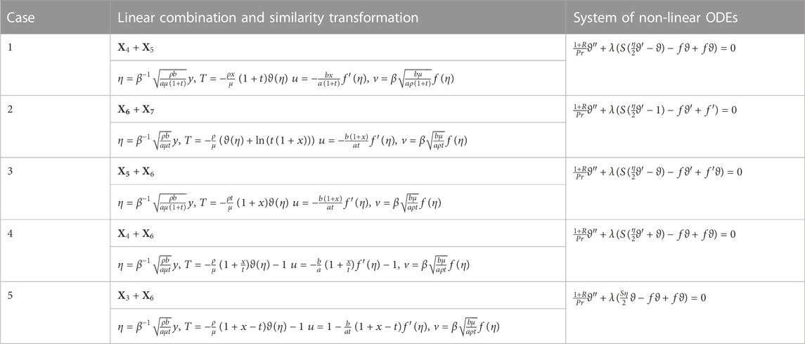
TABLE 2. Lie similarity transformations.

All conditions (2) are transformed to

$f\left(0\right)=0,f^{\prime }\left(0\right)=\vartheta \left(0\right)=1,f\left(1\right)=\frac{S}{2},f^{″}\left(1\right)={\vartheta }^{\prime }\left(1\right)=0.(35)$

By employing these symmetries or their linear combinations, which are again Lie point symmetries, we reduce system (1) twice, using the invariants of these symmetries and their linear combinations. These reductions are in the independent variables of the system, and such double reductions enable the construction of the Lie similarity transformation, as presented in Table 2. This table presents the second transformed equation of (1) obtained through the Lie similarity transformations mentioned previously. The first transformed equation of (1) under all similarity transformations is (34), which is the same for all the systems in Table 2.

3 Numerical solution

The difference equations for a non-linear coupled system of ODEs in (8) are constructed using forward finite difference schemes. We now solve the resulting non-linear algebraic equations obtained along with (9) using the Newton–Raphson method. The boundary conditions at $\eta =0$ and $\eta =1$ are also approximated using forward difference and backward difference finite schemes, respectively. The first-order accurate $O\left(h\right)$ finite-difference approximations for the first-, second-, and third-order derivatives are expressed as follows:

Forward difference:

$\begin{array}{c}\frac{df}{d\eta }=\frac{f\left({\eta }_{i+1}\right)-f\left({\eta }_i\right)}{h},\frac{d^{2}f}{d{\eta }^2}=\frac{f\left({\eta }_{i+2}\right)-2f\left({\eta }_{i+1}\right)+f\left({\eta }_i\right)}{h^2},\hfill \\ \frac{d^{3}f}{d{\eta }^3}=\frac{f\left({\eta }_{i+3}\right)-3f\left({\eta }_{i+2}\right)+3f\left({\eta }_{i+1}\right)-f\left({\eta }_i\right)}{h^3}.\hfill \end{array}(36)$

Backward difference:

$\begin{array}{c}\frac{df}{d\eta }=\frac{f\left({\eta }_i\right)-f\left({\eta }_{i-1}\right)}{h},\frac{d^{2}f}{d{\eta }^2}=\frac{f\left({\eta }_i\right)-2f\left({\eta }_{i-1}\right)+f\left({\eta }_{i-2}\right)}{h^2},\hfill \\ \frac{d^{3}f}{d{\eta }^3}=\frac{f\left({\eta }_{i+3}\right)-3f\left({\eta }_{i+2}\right)+3f\left({\eta }_{i+1}\right)-f\left({\eta }_i\right)}{h^3},\hfill \end{array}(37)$

The resulting non-linear algebraic equations are solved implicitly. If the dimensionless film thickness $\lambda$ in (8) is known, five boundary conditions are required to obtain the solution. However, as $\lambda$ is unknown, the system is made consistent using $f\left(\eta \right)=\frac{S}{2}$ from (9). The system is observed to be stable while obtaining the solutions of the non-linear algebraic equations.

3.1 Convergence and grid independence

Newton’s method was used because of its quadratic convergence rate; however, its convergence strongly depended on the initial guess. We performed iterations with an initial guess of $0.2$ for each term until the error was less than ${10}^{-10}$. For each variable, satisfactory convergence was achieved over approximately $10$ iterations, as shown in Figure 2.

FIGURE 2

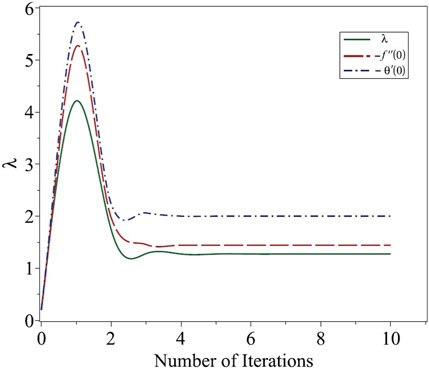
FIGURE 2. Convergence of the numerical solution.

In addition, for all finite-difference-based approximation methods, the truncation error decreased with an increase in the number of nodes. The grid independence was assessed, and a comparison was made with the analytical solution, as shown in Table 3. As the number of nodes exceeds $\mathrm{1,500}$, the $\left|\%\mathrm{e}\mathrm{r}\mathrm{r}\mathrm{o}\mathrm{r}\mathrm{i}\mathrm{n}\beta \right|$ and $\left|\%\mathrm{e}\mathrm{r}\mathrm{r}\mathrm{o}\mathrm{r}\mathrm{i}\mathrm{n}{f}^{″}\left(0\right)\right|$ do not vary significantly. Thus, $\mathrm{1,500}$ nodes were sufficient to approximate the solution of system (8) subject to (9). However, to verify the convergence of the solution in the present study, we approximated all solutions using $\mathrm{2,000}$ nodes.

TABLE 3

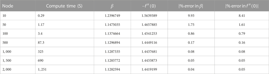
TABLE 3. Variation of the film thickness and skin friction with the number of nodes for FDM at $S=1.2$.

3.2 Validation of the numerical solution method

The numerical results obtained using $\mathrm{2,000}$ nodes were compared with the analytical solutions provided by [8] for the effects of variation of $\lambda$ and $f^{″}\left(0\right)$ as shown in Table 4.

TABLE 4

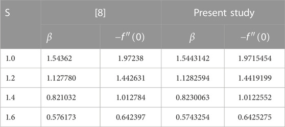
TABLE 4. Validation of the numerical solution using 2,000 nodes with the analytical solution provided by [8].

4 Results and discussion

Five similarity transformations exist for the system of PDEs (1), given in Table 2. The first step is to obtain the approximate solution of the reduced system of ODEs to classify the transformations based on the trends. In this section, we studied the effect of variation of different parameters of flow and heat transfer in the boundary layer. Table 2 indicates that the first equation in all systems (1)–(5) is the same, namely, an uncoupled non-linear ODE with $f\left(\eta \right)$ and $\eta$ as the dependent and independent terms, respectively. Therefore, the variations in film thickness $\lambda$ and velocity distributions $f^{\prime }\left(\eta \right)$ were the same for all these systems, owing to a change in the unsteadiness parameter $S$. In all these systems, the second equation is a coupled non-linear ODE with $f\left(\eta \right)$ and $\vartheta \left(\eta \right)$ as dependent and $\eta$ as independent terms. In the remainder of this section, we first discuss similarity transformations. Subsequently, we study the effects of unsteadiness on film thickness and fluid velocity using the first uncoupled equations of systems (1) and (5). Finally, we present the effects of unsteadiness $S$, Prandtl number $\mathit{Pr}$, and radiation $R$ on the temperature.

4.1 Similarity transformations

A major limitation of the previous similarity transformations for similar types of systems is that they are only valid when $t=1/a$. All previously existing similarity solutions in (7) become invalid at $t=1/a$ because of (3), i.e., $U=bx/\left(1-at\right)$, which dictates the form of these similarity solutions. In a physical sense, these similarity transformations (7) and the resulting system (8) provide a solution in which the velocity of the stretching sheet $U$ is less than the $u$-velocity of the fluid. This limits their applicability to real-world scenarios; however, they form the basis of many real problems, including those addressed in the present study.

However, the similarity solutions for all the systems in the current study obtained using the Lie symmetry transformation and presented in Table 2 have no such limitations. Mathematically, they are all valid at any time (i.e., $t>0$). However, in a physical sense, the velocity and temperature profiles in the boundary layer further finalize the valid transformations. Approximate solutions using a well-established robust method can help eliminate invalid reductions.

4.2 Effects of unsteadiness

Table 5 presents the variation in the dimensionless film thickness $\lambda$ owing to the unsteadiness $S$. For a fully developed flow, the film thickness $\lambda$ decreases with an increase in $S$. Similarly, the velocity of the flow $f^{\prime }\left(\eta \right)$ is directly proportional to $S$ as shown in Figure 3 and Table 5.

TABLE 5

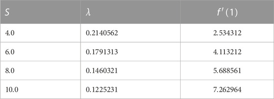
TABLE 5. Variation of the surface velocity and dimensionless film thickness with the unsteadiness parameter.

FIGURE 3

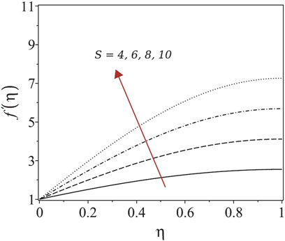
FIGURE 3. Variation of the velocity with the unsteadiness parameter.

Figure 4A; Figure 5A; Figure 6A; Figure 7A show the effects of variation in temperature distribution $\vartheta \left(\eta \right)$ with $S$. For systems (1) and (3), the surface temperature $\vartheta \left(1\right)$ is inversely proportional to $S$, as shown in Table 6. However, the temperatures for systems (4) and (5) increase with $S$. The trends observed for systems (4) and (5) for the variation in $S$ contradict those of incompressible viscous laminar flows because the temperature of fluid $\vartheta \left(\eta \right)$ cannot exceed the temperature of surface $T_s\left(x,t\right)$ or temperature of the flowing fluid itself when the $S$ increases in any fluid flow problem.

FIGURE 4

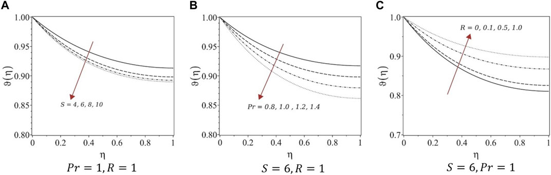
FIGURE 4. Temperature profiles of systems (1) and (3). (A) Pr = 1, R = 1, (B) S = 6, R = 1, and (C) S = 6, Pr = 1.

FIGURE 5

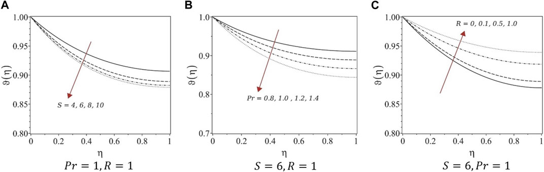
FIGURE 5. Temperature profiles of systems (2). (A) Pr = 1, R = 1, (B) S = 6, R = 1, and (C) S = 6, Pr = 1.

FIGURE 6

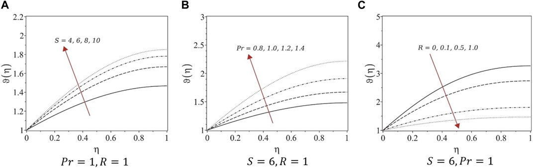
FIGURE 6. Temperature profiles of systems (4). (A) Pr = 1, R = 1, (B) S = 6, R = 1, and (C) S = 6, Pr = 1.

FIGURE 7

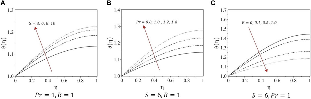
FIGURE 7. Temperature profiles of systems (5). (A) Pr = 1, R = 1, (B) S = 6, R = 1, and (C) S = 6, Pr = 1.

TABLE 6

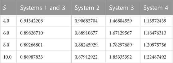
TABLE 6. Variation of the surface temperature with the unsteadiness parameter at $\mathit{Pr}=1$ and $R=1$.

4.3 Effects of the Prandtl number

Figure 4B; Figure 5B; Figure 6B; Figure 7B show the effects of the variation of the Prandtl number $\mathit{Pr}$ on the temperature distribution $\vartheta \left(\eta \right)$ in the boundary layer. For systems (1) and (3), the surface temperature $\vartheta \left(1\right)$ decreases with increasing Prandtl number $\mathit{Pr}$, as shown in Table 7. Similar results have been reported by [16]. However, a decrease in the temperature $\vartheta \left(1\right)$ is observed for systems (4) and (5). The temperature profiles for systems (4) and (5) contradict the trends followed by the incompressible viscous laminar flows obtained for such variations in the Prandtl numbers.

TABLE 7

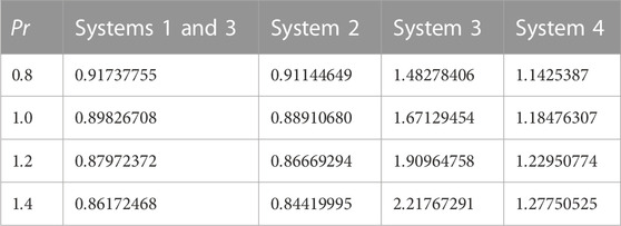
TABLE 7. Variation of the surface temperature with the Prandtl number at $S=6$ and $R=1$.

4.4 Effects of radiation

The effects of the radiation $R$ on the temperature distribution $\vartheta \left(\eta \right)$ in the boundary layer are shown in Figure 4C; Figure 5C; Figure 6C; Figure 7C. As observed before, systems (1) and (3) exhibit trends that are different from the rest of systems (4) and (5); in other words, the surface temperature $\vartheta \left(1\right)$ increases with the $R$ for the first three systems while for systems (4) and (5), it decreases with increasing $R$. In addition, we present the results in Table 8. Liu and Megahed [16] generated temperature profiles by varying $R$ and reported profiles of the type observed for systems (1) and (3). The temperature profiles for systems (4) and (5) contradicted the trends exhibited by the incompressible viscous laminar flows obtained under such variations in radiation. The surface temperature $\vartheta \left(1\right)$ is expected to increase with the radiation in the fluid.

TABLE 8

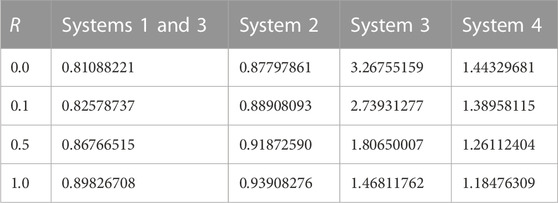
TABLE 8. Variation of the surface temperature with the radiation parameter at $S=6$ and Pr $=1$.

5 Conclusion

We transformed the system of PDEs representing the flow and heat transfer in the boundary layer in the presence of radiation into a system of ODEs using Lie similarity transformations. The Lie similarity transformations presented in this study are different from the existing ones in terms of validity and applicability. These similarity transformations were obtained through invariants associated with linear combinations of Lie symmetry generators, which were used to perform double reductions of the flow model. Four distinct classes of systems of ODEs were revealed with five deduced Lie similarity transformations.

Numerical solutions for the obtained systems of ODEs were determined using finite-difference approximations to eliminate unphysical cases. The first equations in all five systems are the same; hence, the velocity profiles are similar under variations in the unsteadiness parameter. For fully developed flows, the film thickness decreased, whereas the velocity increased with growing unsteadiness. Similar trends were observed for the velocity profiles constructed in this study. For systems (1) and (3), the temperature decreased with increasing unsteadiness and Prandtl number, whereas the temperature increased with increasing radiation parameters. However, for systems (4) and (5), the temperature increased with the unsteadiness parameter and Prandtl number and decreased with increasing the radiation, which is not the case with real fluids. Therefore, we suggest avoiding the similarity transformation of systems (4) and (5) to study similar types of problems.

Overall, the valid similarity solutions determined using an extensive mathematical procedure allowed us to obtain solutions for unsteady fluid flow and heat transfer in the boundary layer. The HAM or homotopy perturbation method can be used to obtain the analytic solutions for the transformed system, providing valid results. The analytic solutions for fully resolved laminar boundary layer flow and heat transfer at any given time can be obtained by inserting the values for appropriate boundary conditions.

Data availability statement

The original contributions presented in the study are included in the article/Supplementary material. Further inquiries can be directed to the corresponding authors.

Author contributions

Conceptualization: MS; data curation: MB; formal analysis: MB, SA, MS, MA, and AZ; software: MB and MS; validation: MB, SA, MS, MA, and AZ; visualization: MB, MS, KK, KK, and JH; writing—original draft preparation: MS and MB; writing—review and editing: SA, KK, MA, AZ, KK, and JH; funding: KK and JH. All authors contributed to the article and approved the submitted version.

Funding

This work was supported by the National Research Foundation of Korea (NRF) grant funded by the Korean government (MSIT) (2022R1C1C2003637 to KK and RS-2023-00210403 to JH).

Conflict of interest

The authors declare that the research was conducted in the absence of any commercial or financial relationships that could be construed as a potential conflict of interest.

Publisher’s note

All claims expressed in this article are solely those of the authors and do not necessarily represent those of their affiliated organizations or those of the publisher, the editors, and the reviewers. Any product that may be evaluated in this article, or claim that may be made by its manufacturer, is not guaranteed or endorsed by the publisher.

References

1. Crane LJ. Flow past a stretching plate. Z für Angew Mathematik Physik ZAMP (1970) 21(4):645–7. doi:10.1007/bf01587695

CrossRef Full Text | Google Scholar

2. Wang C. Liquid film on an unsteady stretching surface. Q Appl Math (1990) 48(4):601–10. doi:10.1090/qam/1079908

CrossRef Full Text | Google Scholar

3. Andersson HI, Aarseth JB, Braud N, Dandapat BS. Flow of a power-law fluid film on an unsteady stretching surface. J Non-Newtonian Fluid Mech (1996) 62(1):1–8. doi:10.1016/0377-0257(95)01392-x

CrossRef Full Text | Google Scholar

4. Andersson HI, Aarseth JB, Dandapat BS. Heat transfer in a liquid film on an unsteady stretching surface. Int J Heat Mass Transfer (2000) 43(1):69–74. doi:10.1016/s0017-9310(99)00123-4

CrossRef Full Text | Google Scholar

5. Chen CH. Heat transfer in a power-law fluid film over a unsteady stretching sheet. Heat Mass Transfer (2003) 39(8):791–6. doi:10.1007/s00231-002-0363-2

CrossRef Full Text | Google Scholar

6. Dandapat BS, Santra B, Andersson HI. Thermocapillarity in a liquid film on an unsteady stretching surface. Int J Heat Mass Transfer (2003) 46(16):3009–15. doi:10.1016/s0017-9310(03)00078-4

CrossRef Full Text | Google Scholar

7. Chen CH. Effect of viscous dissipation on heat transfer in a non-Newtonian liquid film over an unsteady stretching sheet. J Non-Newtonian Fluid Mech (2006) 135(2-3):128–35. doi:10.1016/j.jnnfm.2006.01.009

CrossRef Full Text | Google Scholar

8. Wang C. Analytic solutions for a liquid film on an unsteady stretching surface. Heat Mass Transfer (2006) 42(8):759–66. doi:10.1007/s00231-005-0027-0

CrossRef Full Text | Google Scholar

9. Dandapat B, Santra B, Vajravelu K. The effects of variable fluid properties and thermocapillarity on the flow of a thin film on an unsteady stretching sheet. Int J Heat Mass Transfer (2007) 50(5-6):991–6. doi:10.1016/j.ijheatmasstransfer.2006.08.007

CrossRef Full Text | Google Scholar

10. Liu IC, Andersson HI. Heat transfer in a liquid film on an unsteady stretching sheet. Int J Therm Sci (2008) 47(6):766–72. doi:10.1016/j.ijthermalsci.2007.06.001

CrossRef Full Text | Google Scholar

11. Abel MS, Tawade J, Nandeppanavar MM. Effect of non-uniform heat source on MHD heat transfer in a liquid film over an unsteady stretching sheet. Int J Non-Linear Mech (2009) 44(9):990–8. doi:10.1016/j.ijnonlinmec.2009.07.004

CrossRef Full Text | Google Scholar

12. Aziz RC, Hashim I. Liquid film on unsteady stretching sheet with general surface temperature and viscous dissipation. Chin Phys Lett (2010) 27(11):110202. doi:10.1088/0256-307X/27/11/110202

CrossRef Full Text | Google Scholar

13. Noor NFM, Hashim I. Thermocapillarity and magnetic field effects in a thin liquid film on an unsteady stretching surface. Int J Heat Mass Transfer (2010) 53(9-10):2044–51. doi:10.1016/j.ijheatmasstransfer.2009.12.052

CrossRef Full Text | Google Scholar

14. Aziz RC, Hashim I, Alomari AK. Thin film flow and heat transfer on an unsteady stretching sheet with internal heating. Meccanica (2011) 46(2):349–57. doi:10.1007/s11012-010-9313-0

CrossRef Full Text | Google Scholar

15. Aziz RC, Hashim I, Abbasbandy S. Effects of thermocapillarity and thermal radiation on flow and heat transfer in a thin liquid film on an unsteady stretching sheet. Math Probl Eng (2012) 2012:1–14. doi:10.1155/2012/127320

CrossRef Full Text | Google Scholar

16. Liu IC, Megahed A. Numerical study for the flow and heat transfer in a thin liquid film over an unsteady stretching sheet with variable fluid properties in the presence of thermal radiation. J Mech (2012) 28(2):291–7. doi:10.1017/jmech.2012.32

CrossRef Full Text | Google Scholar

17. Kumar KG. Scrutinization of 3D flow and non-linear radiative heat transfer of non-Newtonian nanoparticles over an exponentially sheet. Int J Numer Methods Heat Fluid Flow (2019) 30:2051–62. doi:10.1108/hff-12-2018-0741

CrossRef Full Text | Google Scholar

18. Kumar KG. Exploration of flow and heat transfer of non-Newtonian nanofluid over a stretching sheet by considering slip factor. Int J Numer Methods Heat Fluid Flow (2019) 30(4):1991–2001. doi:10.1108/hff-11-2018-0687

CrossRef Full Text | Google Scholar

19. Reddy MG, Rani S, Kumar KG, Seikh A, Rahimi-Gorji M, Sherif M. Transverse magnetic flow over a Reiner–Philippoff nanofluid by considering solar radiation. Mod Phys Lett (2019) 33(36):1950449. doi:10.1142/s0217984919504499

CrossRef Full Text | Google Scholar

20. Kumar KG, Hani EH, Assad ME, Rahimi-Gorji M, Nadeem S. A novel approach for investigation of heat transfer enhancement with ferromagnetic hybrid nanofluid by considering solar radiation. Microsystem Tech (2021) 27:97–104. doi:10.1007/s00542-020-04920-8

CrossRef Full Text | Google Scholar

21. Azam M, Abbas N, Ganesh Kumar K, Wali S. Transient bioconvection and activation energy impacts on Casson nanofluid with gyrotactic microorganisms and non-linear radiation. Waves in Random and Complex Media (2022) 1–20. doi:10.1080/17455030.2022.2078014

CrossRef Full Text | Google Scholar

22. Puneeth V, Manjunatha S, Kumar KG, Reddy MG. Perspective of multiple slips on 3D flow of Al₂O₃–TiO₂–CuO/H₂O ternary nanofluid past an extending surface due to non-linear thermal radiation. Waves in Random and Complex Media (2022) 1–19. doi:10.1080/17455030.2022.2041766

CrossRef Full Text | Google Scholar

23. Sudharani MVVNL, Prakasha DG, Kumar KG, Chamkha AJ. Computational assessment of hybrid and tri hybrid nanofluid influenced by slip flow and linear radiation. The Eur Phys J Plus (2023) 138(3):257. doi:10.1140/epjp/s13360-023-03852-2

CrossRef Full Text | Google Scholar

24. Naik LS, Prakasha DG, Praveena MM, Krishnamurthy MR, Kumar KG. Stratification flow and variable heat transfer over different non-Newtonian fluids under the consideration of magnetic dipole. Int J Mod Phys B (2023) 13:2450071. doi:10.1142/s0217979224500711

CrossRef Full Text | Google Scholar

25. Olver PJ. Applications of Lie groups to differential equations. Berlin: Springer Science & Business Media (1993).

Google Scholar

26. Ibragimov NH, Ibragimov NK. Elementary Lie group analysis and ordinary differential equations. New York: Wiley (1999).

Google Scholar

27. Hydon PE. Symmetry methods for differential equations: A beginner's guide. Cambridge, UK: Cambridge University Press (2000).

Google Scholar

28. Safdar M, Khan MI, Taj S, Malik M, Shi QH. Construction of similarity transformations and analytic solutions for a liquid film on an unsteady stretching sheet using lie point symmetries. Chaos, Solitons and Fractals (2021) 150:111115. doi:10.1016/j.chaos.2021.111115

CrossRef Full Text | Google Scholar

29. Bilal M, Safdar M, Taj S, Zafar A, Ali MU, Lee SW. Reduce-order modeling and higher order numerical solutions for unsteady flow and heat transfer in boundary layer with internal heating. Mathematics (2022) 10(24):4640. doi:10.3390/math10244640

CrossRef Full Text | Google Scholar

30. Bilal M, Safdar M, Ahmed S, Riaz AK. Analytic similarity solutions for fully resolved unsteady laminar boundary layer flow and heat transfer in the presence of radiation. Heliyon (2023) 9(4):e14765. doi:10.1016/j.heliyon.2023.e14765

PubMed Abstract | CrossRef Full Text | Google Scholar

31. Raptis A. Flow of a micropolar fluid past a continuously moving plate by the presence of radiation. Int J Heat Mass Transfer (1998) 18(41):2865–6. doi:10.1016/s0017-9310(98)00006-4

CrossRef Full Text | Google Scholar

32. Raptis A. Radiation and viscoelastic flow. Int Commun Heat Mass Transfer (1999) 26(6):889–95. doi:10.1016/s0735-1933(99)00077-9

CrossRef Full Text | Google Scholar