Qubit energy tuner based on single flux quantum circuits

1 Introduction

Josephson qubits with gate and measurement fidelities surpassing the threshold of fault-tolerant quantum computing are attractive candidates for manufacturing scalable quantum computers. Microwave electronics, as a traditional way for qubit control and readout, have succeeded in obtaining gate fidelities beyond 99.9% [1] and realizing quantum supremacy [2]. However, the bottleneck of interconnection becomes significant when the number of qubits increases beyond a thousand due to quantitative restrictions on the input and output ports of the quantum processor and cryogenic transmission lines. It is desirable to introduce single flux quantum (SFQ) digital logic circuits [3] for control and readout [4]to overcome this bottleneck. Digital coherent XY control based on SFQ pulses to transmon qubits was proposed [5], and the fidelities of digital single-qubit gates were measured to be about 95% [6]. Methods of optimization of SFQ pulse sequences for single- [7–9] and two-qubit gates, such as cross-resonance and controlled phase (CZ) gates [10–13], have also been studied.

In order to control qubits with flexibility, SFQ-based devices for Z control have become a frontier that requires further research. McDermott et al. [4] proposed an SFQ-based coprocessor that operates at 3 K for controlling and measuring a quantum processor. This coprocessor requires SFQ-based flux digital-to-analog converters (flux DACs) [14] for Z control, which is an inspiring idea for creating a scalable superconducting quantum processor. Recently, Mohammad et al. [10] proposed an SFQ-based digital controller called DigiQ for superconducting qubits. In DigiQ, the Z control of qubits is performed with bias currents generated by an array of SFQ/DCs. These SFQ/DCs in DigiQ are placed at the 4 K plate of the dilution refrigerator, and bias currents need to be transmitted in superconducting microstrip flex lines to the 10-mK plate where the quantum processor works, which is similar to the approach used in [4].

To further advance the integration of qubits, it is crucial to integrate superconducting SFQ logic circuits for the control and measurement of qubits with quantum processors using 3D integration technologies in future developments [15,16]. Consequently, there is a need to research and design SFQ-based devices for on-chip Z control and ensure that the devices are as simple as possible for scalable quantum processors. These lean devices should be capable of converting SFQ pulse signals into flux signals. The circuits for Z control in DigiQ may be slightly more complex than flux DACs. Therefore, it is intuitive to consider flux DACs as the base for developing SFQ-based devices for Z control. However, the employment of a single flux DAC, as defined in [14], presents challenges in providing flux bias and completing a high-precision Z-control gate simultaneously because of the following reasons: 1) the resetting of a flux DAC at the end of a Z control operation will eliminate not only the flux performing the gate but also the bias flux setting the idle frequency of the controlled qubit and 2) the resetting is achieved by applying Φ₀/2 (half of a flux quantum) to the two-junction reset superconducting quantum interference device (SQUID) loop, which may necessitate another flux DAC, an SFQ/DC, or a coprocessor pin for an external current source. This ultimately increases the physical footprint and complexity of the coprocessor or exacerbates the interconnection bottleneck situation.

Here, we introduce a novel SFQ-based device for Z control, which stems from the improvement of flux DACs. The primary function of the qubit energy tuner (QET) is to adjust the energy levels of qubits. By supplying flux from a QET, the energy levels or frequency of a flux-tunable transmon qubit can be precisely set to specific values. Concurrently, QET enables the execution of gate operations that require flux bias, such as a Z gate or an iSWAP gate. Following a gate operation, the QET can seamlessly return the qubit frequency to its idle state.

The circuit structure of QETs is first presented in Section 2. Then, the key features of a specific QET are analyzed, and a formula is derived to calculate its inductor loop current responsible for providing flux. Section 3 describes the ideal Z control method, which employs square-wave-like currents for flux-tunable transmon. Subsequently, in Section 4, simulations are performed to demonstrate the variation in the inductor loop current of a QET providing flux due to SFQ pulses, as well as the performance of a QET in executing Z and iSWAP gates. Finally, in Section 5, the work is concluded, and the challenges and opportunities associated with QETs in the future are discussed.

2 Structure of the qubit energy tuner

QET comprises an inductor loop and several flux bias units, which can be either positive or negative, as illustrated in Figure 1. The inductor loop is weakly coupled to the SQUID of a flux-tunable transmon, supplying flux for tuning its energy levels. Each flux bias unit includes a Josephson junction shunted with an inductor coupled to the inductor loop. The Josephson junction can be made of an intrinsic Josephson junction in parallel with a resistor to be an overdamped Josephson junction. The node connected to the Josephson junction and the inductor is treated as an input port of QET for the SFQ pulse signal. After receiving an SFQ pulse, a positive flux bias unit increases the external flux through the SQUID by a specific amount, whereas a negative flux bias unit increases it in the opposite direction or decreases it by the same specific amount. This is realized by making the direction of dotted terminals of positive flux bias units the same as that of the corresponding inductor in the inductor loop but making the direction of dotted terminals of negative flux bias units opposite to that of the corresponding inductor in the inductor loop.

FIGURE 1

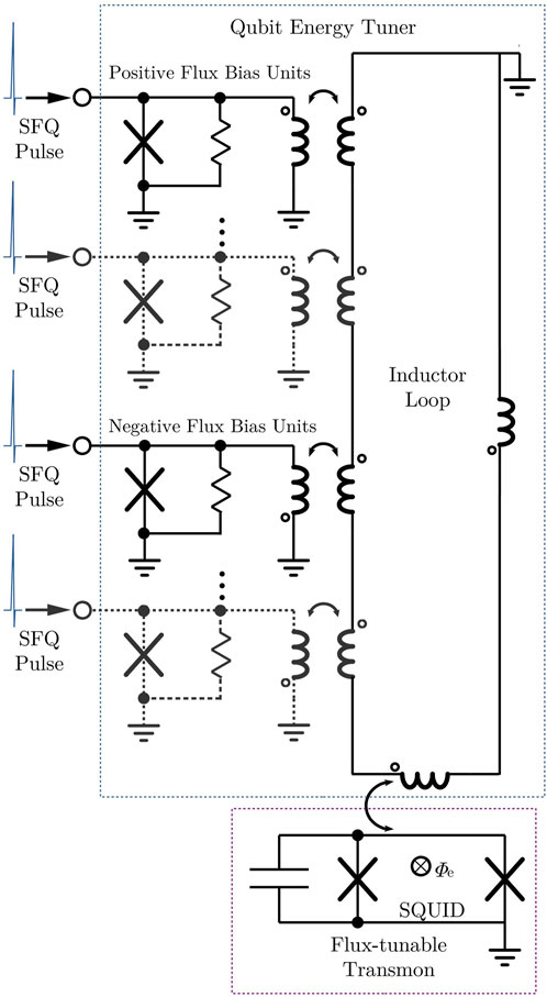
FIGURE 1. Structure of a qubit energy tuner coupled with a flux-tunable transmon.

A QET should have at least a pair of flux bias units, one positive and the other negative. In order to tune the energy levels of a transmon more precisely, QET can be designed to have two or more pairs of flux bias units, among which some pairs are used for coarse tuning and others are used for fine-tuning. Inductors in different flux bias units can be coupled. The inspiration for the QET is from the design of the flux DAC proposed in [14] and [17]. Therefore, its circuits have similar but simpler structures compared with those of flux DACs.

The QET shown in Figure 2 is an example of the following analysis. It has a pair of flux bias units for coarse tuning and another pair for fine-tuning. The parameters of elements in the example are listed in Table 2. The symbol for QET in Figure 2 is drawn as in Figure 3. This kind of QET with two pairs of flux bias units is chosen to be analyzed because it combines accuracy, simplicity, and speed better than other cases with only one or over two pairs of flux bias units. On one hand, the QET with only a pair of flux bias units has only one precision, which causes a low speed of high-precision tuning or a low precision of high-speed tuning. On the other hand, the QET with three or more pairs of flux bias units has more ports and circuit elements, which means more complicated control, reduced reliability, and a larger footprint.

FIGURE 2

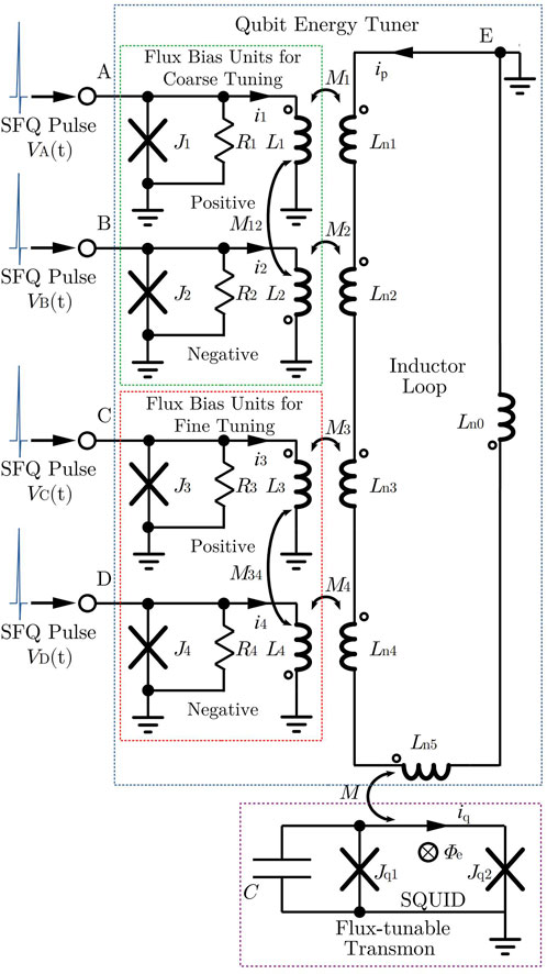
FIGURE 2. Schematic representation of a qubit energy tuner with two pairs of flux bias units for coarse tuning and fine-tuning.

FIGURE 3

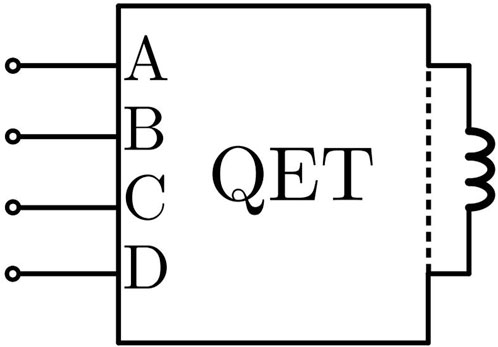
FIGURE 3. Symbol of a QET.

According to Kirchhoff’s voltage law, the electric potentials of nodes A, B, C, D, and E in Figure 2 are

$V_{\text{A}}\left(t^{\prime }\right)=L_1\frac{\mathrm{d}{i}_1\left(t^{\prime }\right)}{\mathrm{d}{t}^{\prime }}+M_1\frac{\mathrm{d}{i}_{\text{p}}\left(t^{\prime }\right)}{\mathrm{d}{t}^{\prime }}+M_{12}\frac{\mathrm{d}{i}_2\left(t^{\prime }\right)}{\mathrm{d}{t}^{\prime }},(1)$

$V_{\text{B}}\left(t^{\prime }\right)=L_2\frac{\mathrm{d}{i}_2\left(t^{\prime }\right)}{\mathrm{d}{t}^{\prime }}-M_2\frac{\mathrm{d}{i}_{\text{p}}\left(t^{\prime }\right)}{\mathrm{d}{t}^{\prime }}+M_{12}\frac{\mathrm{d}{i}_1\left(t^{\prime }\right)}{\mathrm{d}{t}^{\prime }},(2)$

$V_{\text{C}}\left(t^{\prime }\right)=L_3\frac{\mathrm{d}{i}_3\left(t^{\prime }\right)}{\mathrm{d}{t}^{\prime }}+M_3\frac{\mathrm{d}{i}_{\text{p}}\left(t^{\prime }\right)}{\mathrm{d}{t}^{\prime }}+M_{34}\frac{\mathrm{d}{i}_4\left(t^{\prime }\right)}{\mathrm{d}{t}^{\prime }},(3)$

$V_{\text{D}}\left(t^{\prime }\right)=L_4\frac{\mathrm{d}{i}_4\left(t^{\prime }\right)}{\mathrm{d}{t}^{\prime }}-M_4\frac{\mathrm{d}{i}_{\text{p}}\left(t^{\prime }\right)}{\mathrm{d}{t}^{\prime }}+M_{34}\frac{\mathrm{d}{i}_3\left(t^{\prime }\right)}{\mathrm{d}{t}^{\prime }},(4)$

$\begin{array}{cc}\hfill V_{\text{E}}\left(t^{\prime }\right)& =L_{\mathrm{\Sigma }}\frac{\mathrm{d}{i}_{\text{p}}\left(t^{\prime }\right)}{\mathrm{d}{t}^{\prime }}+M_1\frac{\mathrm{d}{i}_1\left(t^{\prime }\right)}{\mathrm{d}{t}^{\prime }}-M_2\frac{\mathrm{d}{i}_2\left(t^{\prime }\right)}{\mathrm{d}{t}^{\prime }}\hfill \\ \hfill & +M_3\frac{\mathrm{d}{i}_3\left(t^{\prime }\right)}{\mathrm{d}{t}^{\prime }}-M_4\frac{\mathrm{d}{i}_4\left(t^{\prime }\right)}{\mathrm{d}{t}^{\prime }}+M\frac{\mathrm{d}{i}_{\text{q}}\left(t^{\prime }\right)}{\mathrm{d}{t}^{\prime }},\hfill \end{array}(5)$

where

$L_{\mathrm{\Sigma }}=L_{\text{n0}}+L_{\text{n}1}+L_{\text{n}2}+L_{\text{n}3}+L_{\text{n}4}+L_{\text{n}5}(6)$

is the total inductance of the inductor loop obtained by summing self-inductances of all parts of the inductor loop. L₁, L₂, L₃, and L₄ are self-inductances of inductors in flux bias units. M₁, M₂, M₃, and M₄ are mutual inductances of flux bias units and the inductor loop, as shown in Figure 2. M is the mutual inductance between the inductor loop and the SQUID of flux-tunable transmon. i₁ (t′), i₂ (t′), i₃ (t′), and i₄ (t′) are currents of inductors in flux bias units at the moment t′. i_p (t′) and i_q (t′) are the currents of the inductor loop and the SQUID at the moment t′.

Under the zero initial condition, integrating both sides of Eqs 1–5 with 0 as the lower bound and time t as the upper bound yields

${\int }_0^t{V}_{\text{A}}\left(t^{\prime }\right)\mathrm{d}{t}^{\prime }=L_1{i}_1\left(t\right)+M_1{i}_{\text{p}}\left(t\right)+M_{12}{i}_2\left(t\right),(7)$

${\int }_0^t{V}_{\text{B}}\left(t^{\prime }\right)\mathrm{d}{t}^{\prime }=L_2{i}_2\left(t\right)-M_2{i}_{\text{p}}\left(t\right)+M_{12}{i}_1\left(t\right),(8)$

${\int }_0^t{V}_{\text{C}}\left(t^{\prime }\right)\mathrm{d}{t}^{\prime }=L_3{i}_3\left(t\right)+M_3{i}_{\text{p}}\left(t\right)+M_{34}{i}_4\left(t\right),(9)$

${\int }_0^t{V}_{\text{D}}\left(t^{\prime }\right)\mathrm{d}{t}^{\prime }=L_4{i}_4\left(t\right)-M_4{i}_{\text{p}}\left(t\right)+M_{34}{i}_3\left(t\right),(10)$

$\begin{array}{cc}\hfill {\int }_0^t{V}_{\mathrm{E}}\left(t^{\prime }\right)\mathrm{d}{t}^{\prime }& =L_{\mathrm{\Sigma }}{i}_{\text{p}}\left(t\right)+M_1{i}_1\left(t\right)-M_2{i}_2\left(t\right)\hfill \\ \hfill & +M_3{i}_3\left(t\right)-M_4{i}_4\left(t\right)+M{i}_{\text{q}}\left(t\right).\hfill \end{array}(11)$

The mutual inductance M is designed to be much smaller than the total inductance of the inductor loop L_Σ and other mutual inductances like M₁ for weak coupling to the SQUID of the qubit. Additionally, the ring current of the SQUID i_q(t) should be less than the critical current of its Josephson junctions, which is about tens of nA for Al/AlOx/Al junctions and smaller than the current in the inductance loop i_p(t) (about several or tens of mA) by two or more orders of magnitude. Therefore, the influence of the SQUID on the inductance loop, Mi_q, can be ignored in Eq. 11, and the electric potential of node E is rewritten as

$\begin{array}{cc}\hfill {\int }_0^t{V}_{\mathrm{E}}\left(t^{\prime }\right)\mathrm{d}{t}^{\prime }& =L_{\mathrm{\Sigma }}{i}_{\text{p}}\left(t\right)+M_1{i}_1\left(t\right)-M_2{i}_2\left(t\right)\hfill \\ \hfill & +M_3{i}_3\left(t\right)-M_4{i}_4\left(t\right).\hfill \end{array}(12)$

Then, let

${\Phi }_{\text{A}}\left(t\right)={\int }_0^t{V}_{\text{A}}\left(t^{\prime }\right)\mathrm{d}{t}^{\prime },(13)$

${\Phi }_{\text{B}}\left(t\right)={\int }_0^t{V}_{\text{B}}\left(t^{\prime }\right)\mathrm{d}{t}^{\prime },(14)$

${\Phi }_{\text{C}}\left(t\right)={\int }_0^t{V}_{\text{C}}\left(t^{\prime }\right)\mathrm{d}{t}^{\prime },(15)$

${\Phi }_{\text{D}}\left(t\right)={\int }_0^t{V}_{\text{D}}\left(t^{\prime }\right)\mathrm{d}{t}^{\prime },(16)$

${\Phi }_{\text{E}}\left(t\right)={\int }_0^t{V}_{\text{E}}\left(t^{\prime }\right)\mathrm{d}{t}^{\prime },(17)$

and we get

$\mathit{\Phi }\left(t\right)=\mathit{L}\mathit{i}\left(t\right),(18)$

where

$\mathit{\Phi }\left(t\right)=\left[\begin{array}{c}\hfill {\Phi }_{\text{A}}\left(t\right)\hfill \\ \hfill {\Phi }_{\text{B}}\left(t\right)\hfill \\ \hfill {\Phi }_{\text{C}}\left(t\right)\hfill \\ \hfill {\Phi }_{\text{D}}\left(t\right)\hfill \\ \hfill {\Phi }_{\text{E}}\left(t\right)\hfill \end{array}\right],(19)$

$\mathit{i}\left(t\right)=\left[\begin{array}{c}\hfill i_1\left(t\right)\hfill \\ \hfill i_2\left(t\right)\hfill \\ \hfill i_3\left(t\right)\hfill \\ \hfill i_4\left(t\right)\hfill \\ \hfill i_{\text{p}}\left(t\right)\hfill \end{array}\right],(20)$

and

$\mathit{L}=\left[\begin{array}{ccccc}\hfill L_1\hfill & \hfill M_{12}\hfill & \hfill 0\hfill & \hfill 0\hfill & \hfill M_1\hfill \\ \hfill M_{12}\hfill & \hfill L_2\hfill & \hfill 0\hfill & \hfill 0\hfill & \hfill -M_2\hfill \\ \hfill 0\hfill & \hfill 0\hfill & \hfill L_3\hfill & \hfill M_{34}\hfill & \hfill M_3\hfill \\ \hfill 0\hfill & \hfill 0\hfill & \hfill M_{34}\hfill & \hfill L_4\hfill & \hfill -M_4\hfill \\ \hfill M_1\hfill & \hfill -M_2\hfill & \hfill M_3\hfill & \hfill -M_4\hfill & \hfill L_{\mathrm{\Sigma }}\hfill \end{array}\right].(21)$

Then, to get i(t), we have

$\mathit{i}\left(t\right)={\mathit{L}}^{-1}\mathit{\Phi }\left(t\right),(22)$

where ${\mathit{L}}^{-1}=\frac{1}{F}\mathit{A}$. $\frac{1}{F}$ is the common factor of the elements in the inverse matrix of L. F is

$\begin{array}{cc}\hfill F& =L_2\left(M_{34}^2\left(L_1{L}_{\mathrm{\Sigma }}-M_1^2\right)+2L_1{M}_3{M}_{34}{M}_4\right.\hfill \\ \hfill & \left.+L_3\left(-L_4\left(L_1{L}_{\mathrm{\Sigma }}-M_1^2\right)+L_1{M}_4^2\right)+L_1{L}_4{M}_3^2\right)\hfill \\ \hfill & +\left(-L_1{M}_2^2-L_{\mathrm{\Sigma }}{M}_{12}^2-2M_1{M}_{12}{M}_2\right)M_{34}^2\hfill \\ \hfill & -2M_{12}^2{M}_3{M}_{34}{M}_4\hfill \\ \hfill & +L_3\left(\left(L_1{M}_2^2+L_{\mathrm{\Sigma }}{M}_{12}^2+2M_1{M}_{12}{M}_2\right)L_4-M_{12}^2{M}_4^2\right)\hfill \\ \hfill & -L_4{M}_{12}^2{M}_3^2.\hfill \end{array}(23)$

The elements a_ij (i, j = 1, 2, 3, 4, 5) of A are

$\begin{array}{ccc}\hfill a_{11}& =\hfill & L_2\left(M_{34}^2{L}_{\mathrm{\Sigma }}+2M_3{M}_4{M}_{34}\right.\hfill \\ \hfill & \hfill & \left.+\left(-L_4{L}_{\mathrm{\Sigma }}+M_4^2\right)L_3+L_4{M}_3^2\right)\hfill \\ \hfill & \hfill & +M_2^2\left(L_3{L}_4-M_{34}^2\right),\hfill \\ \hfill a_{12}& =\hfill & M_{12}\left(-M_{34}^2{L}_{\mathrm{\Sigma }}-2M_3{M}_4{M}_{34}\right.\hfill \\ \hfill & \hfill & \left.+\left(L_4{L}_{\mathrm{\Sigma }}-M_4^2\right)L_3-L_4{M}_3^2\right)\hfill \\ \hfill & \hfill & +M_1{M}_2\left(L_3{L}_4-M_{34}^2\right),\hfill \\ \hfill a_{13}& =\hfill & -\left(L_4{M}_3+M_{34}{M}_4\right)\left(L_2{M}_1+M_{12}{M}_2\right),\hfill \\ \hfill a_{14}& =\hfill & \left(L_2{M}_1+M_{12}{M}_2\right)\left(L_3{M}_4+M_3{M}_{34}\right),\hfill \\ \hfill a_{15}& =\hfill & \left(L_3{L}_4-M_{34}^2\right)\left(L_2{M}_1+M_{12}{M}_2\right),\hfill \\ \hfill & \hfill & \hfill \\ \hfill a_{21}& =\hfill & M_{12}\left(-M_{34}^2{L}_{\mathrm{\Sigma }}-2M_3{M}_4{M}_{34}\right.\hfill \\ \hfill & \hfill & \left.+\left(L_4{L}_{\mathrm{\Sigma }}-M_4^2\right)L_3-L_4{M}_3^2\right)\hfill \\ \hfill & \hfill & +M_1{M}_2\left(L_3{L}_4-M_{34}^2\right),\hfill \\ \hfill a_{22}& =\hfill & L_1\left(M_{34}^2{L}_{\mathrm{\Sigma }}+2M_3{M}_4{M}_{34}\right.\hfill \\ \hfill & \hfill & \left.+\left(-L_4{L}_{\mathrm{\Sigma }}+M_4^2\right)L_3+L_4{M}_3^2\right)\hfill \\ \hfill & \hfill & +M_1^2\left(L_3{L}_4-M_{34}^2\right),\hfill \\ \hfill a_{23}& =\hfill & \left(L_4{M}_3+M_{34}{M}_4\right)\left(L_1{M}_2+M_1{M}_{12}\right),\hfill \\ \hfill a_{24}& =\hfill & -\left(L_1{M}_2+M_1{M}_{12}\right)\left(L_3{M}_4+M_3{M}_{34}\right),\hfill \\ \hfill a_{25}& =\hfill & -\left(L_3{L}_4-M_{34}^2\right)\left(L_1{M}_2+M_1{M}_{12}\right),\hfill \\ \hfill & \hfill & \hfill \\ \hfill a_{31}& =\hfill & -\left(L_4{M}_3+M_{34}{M}_4\right)\left(L_2{M}_1+M_{12}{M}_2\right),\hfill \\ \hfill a_{32}& =\hfill & \left(L_4{M}_3+M_{34}{M}_4\right)\left(L_1{M}_2+M_1{M}_{12}\right),\hfill \\ \hfill a_{33}& =\hfill & L_4\left(L_{\mathrm{\Sigma }}{M}_{12}^2+2M_1{M}_2{M}_{12}\right.\hfill \\ \hfill & \hfill & \left.+\left(-L_2{L}_{\mathrm{\Sigma }}+M_2^2\right)L_1+L_2{M}_1^2\right)\hfill \\ \hfill & \hfill & +M_4^2\left(L_1{L}_2-M_{12}^2\right),\hfill \\ \hfill a_{34}& =\hfill & M_{34}\left(-L_{\mathrm{\Sigma }}{M}_{12}^2-2M_1{M}_2{M}_{12}\right.\hfill \\ \hfill & \hfill & \left.+\left(L_2{L}_{\mathrm{\Sigma }}-M_2^2\right)L_1-L_2{M}_1^2\right)\hfill \\ \hfill & \hfill & +M_3{M}_4\left(L_1{L}_2-M_{12}^2\right),\hfill \\ \hfill a_{35}& =\hfill & \left(L_1{L}_2-M_{12}^2\right)\left(L_4{M}_3+M_{34}{M}_4\right),\hfill \end{array}$

$\begin{array}{ccc}\hfill a_{41}& =\hfill & \left(L_2{M}_1+M_{12}{M}_2\right)\left(L_3{M}_4+M_3{M}_{34}\right),\hfill \\ \hfill a_{42}& =\hfill & -\left(L_1{M}_2+M_1{M}_{12}\right)\left(L_3{M}_4+M_3{M}_{34}\right),\hfill \\ \hfill a_{43}& =\hfill & M_{34}\left(-L_{\mathrm{\Sigma }}{M}_{12}^2-2M_1{M}_2{M}_{12}\right.\hfill \\ \hfill & \hfill & \left.+\left(L_2{L}_{\mathrm{\Sigma }}-M_2^2\right)L_1-L_2{M}_1^2\right)\hfill \\ \hfill & \hfill & +M_3{M}_4\left(L_1{L}_2-M_{12}^2\right),\hfill \\ \hfill a_{44}& =\hfill & L_3\left(L_{\mathrm{\Sigma }}{M}_{12}^2+2M_1{M}_2{M}_{12}\right.\hfill \\ \hfill & \hfill & \left.+\left(-L_2{L}_{\mathrm{\Sigma }}+M_2^2\right)L_1+L_2{M}_1^2\right)\hfill \\ \hfill & \hfill & +M_3^2\left(L_1{L}_2-M_{12}^2\right),\hfill \\ \hfill a_{45}& =\hfill & -\left(L_1{L}_2-M_{12}^2\right)\left(L_3{M}_4+M_3{M}_{34}\right),\hfill \\ \hfill & \hfill & \hfill \\ \hfill a_{51}& =\hfill & \left(L_3{L}_4-M_{34}^2\right)\left(L_2{M}_1+M_{12}{M}_2\right),\hfill \\ \hfill a_{52}& =\hfill & -\left(L_3{L}_4-M_{34}^2\right)\left(L_1{M}_2+M_1{M}_{12}\right),\hfill \\ \hfill a_{53}& =\hfill & \left(L_1{L}_2-M_{12}^2\right)\left(L_4{M}_3+M_{34}{M}_4\right),\hfill \\ \hfill a_{54}& =\hfill & -\left(L_1{L}_2-M_{12}^2\right)\left(L_3{M}_4+M_3{M}_{34}\right),\hfill \\ \hfill a_{55}& =\hfill & -\left(L_3{L}_4-M_{34}^2\right)\left(L_1{L}_2-M_{12}^2\right).\hfill \end{array}$

Therefore, we have

$\begin{array}{cc}\hfill i_{\text{p}}\left(t\right)=& \frac{1}{F}\left(a_{51}{\Phi }_{\text{A}}\left(t\right)+a_{52}{\Phi }_{\text{B}}\left(t\right)\right.\hfill \\ \hfill & \left.+a_{53}{\Phi }_{\text{C}}\left(t\right)+a_{54}{\Phi }_{\text{D}}\left(t\right)+a_{55}{\Phi }_{\text{E}}\left(t\right)\right),\hfill \end{array}(26)$

that is,

$\begin{array}{cc}\hfill i_{\text{p}}\left(t\right)=& \frac{1}{F}\left({\Phi }_{\text{A}}\left(t\right)\left(L_3{L}_4-M_{34}^2\right)\left(L_2{M}_1+M_{12}{M}_2\right)\right.\hfill \\ \hfill & -{\Phi }_{\text{B}}\left(t\right)\left(L_3{L}_4-M_{34}^2\right)\left(L_1{M}_2+M_1{M}_{12}\right)\hfill \\ \hfill & +{\Phi }_{\text{C}}\left(t\right)\left(L_1{L}_2-M_{12}^2\right)\left(L_4{M}_3+M_{34}{M}_4\right)\hfill \\ \hfill & -{\Phi }_{\text{D}}\left(t\right)\left(L_1{L}_2-M_{12}^2\right)\left(L_3{M}_4+M_3{M}_{34}\right)\hfill \\ \hfill & \left.-{\Phi }_{\text{E}}\left(t\right)\left(L_3{L}_4-M_{34}^2\right)\left(L_1{L}_2-M_{12}^2\right)\right).\hfill \end{array}(27)$

Because node E is connected to the ground, Φ_E should always be zero. In order to make the flux bias units of coarse tuning be able to increase or decrease the external flux through the SQUID by the same amount, the following requirements should be met:

$L_1=L_2=L_{\text{c}},(\mathrm{28a})$

$M_1=M_2=M_{\text{c}}.(\mathrm{28b})$

Similarly, for the flux bias units of fine-tuning, we have

$L_3=L_4=L_{\text{f}},(\mathrm{29a})$

$M_3=M_4=M_{\text{f}}.(\mathrm{29b})$

Therefore, i_p(t) becomes

$\begin{array}{cc}\hfill i_{\text{p}}\left(t\right)=& \frac{1}{F}\left[\left({\Phi }_{\text{A}}-{\Phi }_{\text{B}}\right)\left(L_{\text{f}}^2-M_{34}^2\right)\left(L_{\text{c}}+M_{12}\right)M_{\text{c}}\right.\hfill \\ \hfill & \left.+\left({\Phi }_{\text{C}}-{\Phi }_{\text{D}}\right)\left(L_{\text{c}}^2-M_{12}^2\right)\left(L_{\text{f}}+M_{34}\right)M_{\text{f}}\right],\hfill \end{array}(30)$

where Φ_A, Φ_B, Φ_C, and Φ_D are the integral of the voltage at nodes A, B, C, and D over time t, respectively. Because the input signal to these nodes is SFQ, Φ_A, Φ_B, Φ_C, and Φ_D are multiples of flux quantum Φ₀. F becomes

$\begin{array}{cc}\hfill F& =L_{\text{c}}{L}_{\text{f}}\left(\left(-L_{\mathrm{\Sigma }}{L}_{\text{f}}+M_{\text{f}}^2\right)L_{\text{c}}+L_{\text{f}}{M}_{\text{c}}^2\right)\hfill \\ \hfill & +\left(L_{\text{f}}+M_{34}\right)\left(L_{\mathrm{\Sigma }}{L}_{\text{f}}-L_{\mathrm{\Sigma }}{M}_{34}-2M_{\text{f}}^2\right)M_{12}^2\hfill \\ \hfill & +\left(2L_{\text{f}}^2{M}_{\text{c}}^2-2M_{34}^2{M}_{\text{c}}^2\right)M_{12}\hfill \\ \hfill & +L_{\text{c}}\left(\left(L_{\mathrm{\Sigma }}{L}_{\text{c}}-2M_{\text{c}}^2\right)M_{34}^2\right.\hfill \\ \hfill & \left.+2L_{\text{c}}{M}_{\text{f}}{M}_{\text{f}}{M}_{34}+L_{\text{c}}{L}_{\text{f}}{M}_{\text{f}}^2+L_{\text{f}}^2{M}_{\text{c}}^2\right).\hfill \end{array}(31)$

Hence, the relationship between the current of the inductor loop i_p(t) and the external flux through the SQUID Φ_e is

${\Phi }_{\text{e}}=M{i}_{\text{p}}\left(t\right).(32)$

Denoting

${\Phi }_{\text{A}}-{\Phi }_{\text{B}}=n_{\text{c}}{\mathrm{\Phi }}_0,(33)$

${\Phi }_{\text{C}}-{\Phi }_{\text{D}}=n_{\text{f}}{\mathrm{\Phi }}_0,(34)$

$\frac{M}{F}\left(L_{\text{f}}^2-M_{34}^2\right)\left(L_{\text{c}}+M_{12}\right)M_{\text{c}}=r_{\text{c}},(35)$

$\frac{M}{F}\left(L_{\text{c}}^2-M_{12}^2\right)\left(L_{\text{f}}+M_{34}\right)M_{\text{f}}=r_{\text{f}},(36)$

$\frac{1}{F}\left(L_{\text{f}}^2-M_{34}^2\right)\left(L_{\text{c}}+M_{12}\right)M_{\text{c}}{\mathrm{\Phi }}_0=\mathrm{\Delta }{i}_{\text{pc}},(37)$

$\frac{1}{F}\left(L_{\text{c}}^2-M_{12}^2\right)\left(L_{\text{f}}+M_{34}\right)M_{\text{f}}{\mathrm{\Phi }}_0=\mathrm{\Delta }{i}_{\text{pf}},(38)$

$M\mathrm{\Delta }{i}_{\text{pc}}={\Phi }_{\text{ec}},(39)$

$M\mathrm{\Delta }{i}_{\text{pf}}={\Phi }_{\text{ef}}(40)$

yields

$i_{\text{p}}=n_{\text{c}}\mathrm{\Delta }{i}_{\text{pc}}+n_{\text{f}}\mathrm{\Delta }{i}_{\text{pf}},(41)$

${\Phi }_{\text{e}}=n_{\text{c}}{\Phi }_{\text{ec}}+n_{\text{f}}{\Phi }_{\text{ef}},(42)$

${\Phi }_{\text{ec}}=r_{\text{c}}{\mathrm{\Phi }}_0,(43)$

${\Phi }_{\text{ef}}=r_{\text{f}}{\mathrm{\Phi }}_0.(44)$

Eqs 42–44 mean that the flux provided by QET can be divided into two parts, n_cΦ_ec and n_fΦ_ef, which are, respectively, created by coarse tuning and fine-tuning. Φ_ec can be regarded as the flux unit of coarse tuning, and Φ_ef can be regarded as the flux unit of fine-tuning. If n_c (or n_f) SFQ pulses are inputted to port A (or C) of the QET, then the external flux through the SQUID will increase by n_c times of Φ_ec (or n_f times of Φ_ef). Subsequently, if this external flux needs to be eliminated, n_c (or n_f) SFQ pulses should be inputted to port B (or D). Usually, for fine-tuning, r_f is smaller than r_c. If

$L_{\text{c}}=L_1=L_{\text{n}1}=L_2=L_{\text{n}2},(45)$

$L_{\text{f}}=L_3=L_{\text{n}3}=L_4=L_{\text{n}4},(46)$

then the ratio of the flux unit of coarse tuning to the flux unit of fine-tuning can be defined as

$r_{\text{cf}}=\frac{{\Phi }_{\text{ec}}}{{\Phi }_{\text{ef}}}.(47)$

With Eq. 33 ∼Eq. 47, there is

$r_{\text{cf}}=\frac{r_{\text{c}}}{r_{\text{f}}}=\frac{\mathrm{\Delta }{i}_{\text{pc}}}{\mathrm{\Delta }{i}_{\text{pf}}}=\frac{K_{\text{c}}\left(1-K_{34}\right)}{K_{\text{f}}\left(1-K_{12}\right)},(48)$

where the coupling coefficients are

$K_{\text{c}}=\frac{M_{\text{c}}}{\sqrt{L_1{L}_{\text{n}1}}}=\frac{M_{\text{c}}}{\sqrt{L_2{L}_{\text{n}2}}}=\frac{M_{\text{c}}}{L_{\text{c}}},(49)$

$K_{\text{f}}=\frac{M_{\text{f}}}{\sqrt{L_1{L}_{\text{n}1}}}=\frac{M_{\text{f}}}{\sqrt{L_2{L}_{\text{n}2}}}=\frac{M_{\text{f}}}{L_{\text{f}}},(50)$

$K_{12}=\frac{M_{12}}{\sqrt{L_1{L}_2}}=\frac{M_{12}}{L_{\text{c}}},(51)$

$K_{34}=\frac{M_{34}}{\sqrt{L_3{L}_4}}=\frac{M_{34}}{L_{\text{f}}}.(52)$

The parameter r_cf indicates the ratio of the flux precision of coarse tuning to that of fine-tuning. It should have an appropriate value greater than 1, like 10, to distinguish the two precisions. The parameter r_f is the ratio of the smallest variation of the flux Φ_e, Φ_ef, to flux quantum Φ₀; it determines the flux precision of fine-tuning. The parameter r_c is the ratio of Φ_ec to flux quantum Φ₀ and can be set by r_c = r_cf ⋅ r_f.

The parameters r_cf, r_f, and r_c are the main concerns and should be first determined to design a QET. Then, with constraints including Eqs 35, 36, 45, 46, 48 ∼Eq. 52, all parameter values of circuit elements should be tried and iterated to meet the requirements from the higher-level design; for example, the footprint of the QET on the chip is matched with the footprint of the qubit.

A QET has almost zero static power dissipation in theory because no current will flow through its resistors when Josephson junctions are not switched. Assuming that a QET is used for a gate operation per 20 ns and about 20 SFQ pulses are required for each gate operation, the average switching frequency of Josephson junctions in the QET, f_s, is about 1 GHz. With the critical current I_C = 160 μA and a flux quantum Φ₀ ≈ 2.06783385 × 10⁻¹⁵Wb, the dynamic power dissipation P_D of a QET can be estimated to be 0.33 nW according to the following formula [18]:

$P_{\text{D}}=f_{\text{s}}{\Phi }_0{I}_{\text{C}}.(53)$

3 Ideal Z control by square-wave-like currents

In order to simplify the analysis and understand the main factors affecting the results of Z control, the square-wave-like waveforms of currents producing external flux Φ_e are considered as the ideal cases for a flux-tunable transmon. This section reviewed and discussed how the ideal Z control is performed.

The Hamiltonian of a flux-tunable transmon [19] is

$\widehat{H}=4E_{\text{C}}{\left(\widehat{n}-n_{\text{g}}\right)}^2-E_{\text{JS}}\left({\phi }_{\text{e}}\right)\cos \left(\widehat{\varphi }\right),(54)$

where

$E_{\text{JS}}\left({\phi }_{\text{e}}\right)=E_{\text{J}\mathrm{\Sigma }}|\cos \left({\phi }_{\text{e}}\right)|\sqrt{1+d^2{\tan }^2\left({\phi }_{\text{e}}\right)}(55)$

is the effective Josephson energy of the SQUID of the transmon with a total Josephson coupling energy of two junctions

$E_{\text{J}\mathrm{\Sigma }}=E_{\text{J}1}+E_{\text{J}2},(56)$

an asymmetry coefficient

$d=\frac{E_{\text{J}2}-E_{\text{J}1}}{E_{\text{J}\mathrm{\Sigma }}},(57)$

and a reduced external flux

${\phi }_{\text{e}}=\pi \frac{{\Phi }_{\text{e}}\left(t\right)}{{\mathrm{\Phi }}_0}.(58)$

E_C is the charging energy of the transmon. n_g is the effective offset charge. $\widehat{n}$ and $\widehat{\varphi }$ are, respectively, the number operator and the phase operator of Cooper pairs. For convenience, the hats of all operators, including Hamiltonian, are left out in the following derivation.

The solution for the k^th eigen energy of Eq. 54 with the first-order approximation of perturbation theory [19] is

$E_k=k\sqrt{8E_{\text{C}}{E}_{\text{JS}}\left({\phi }_{\text{e}}\right)}-\frac{E_{\text{C}}}{12}\left(6k^2+6k+3\right)-E_{\text{JS}}\left({\phi }_{\text{e}}\right).(59)$

Usually, the external flux Φ_e(t) at the moment t for Z control is provided by a conductor line beside the SQUID with its current, i_z(t), and a mutual inductance between the line and the SQUID, M. Because the current in the SQUID is much smaller than i_z(t), its influence on i_z(t) can be ignored. There is

${\Phi }_{\text{e}}\left(t\right)=M{i}_{\text{z}}\left(t\right).(60)$

Therefore, E_JS (φ_e) can be written as

$E_{\text{JS}}\left(i_{\text{z}}\left(t\right)\right)=E_{\text{J}\mathrm{\Sigma }}\left|\cos \left(\pi \frac{M{i}_{\text{z}}\left(t\right)}{{\mathrm{\Phi }}_0}\right)\right|\sqrt{1+d^2{\tan }^2\left(\pi \frac{M{i}_{\text{z}}\left(t\right)}{{\mathrm{\Phi }}_0}\right)}.(61)$

By changing i_z(t), E_JS (i_z(t)) can be set to a target value. Then, the energy level E_k, especially E₀ and E₁, can be tuned so that the qubit frequency is set to the corresponding target value. When E_JS (i_z(t)) is set, the condition E_JS (i_z(t))/E_C ≫ 1 should be guaranteed to make sure that the qubit is a transmon. According to Eq. 59, we have

$E_0=-\frac{E_{\text{C}}}{4}-E_{\text{JS}}\left({\phi }_{\text{e}}\right),(62)$

$E_1=\sqrt{8E_{\text{C}}{E}_{\text{JS}}\left({\phi }_{\text{e}}\right)}-E_{\text{C}}-\frac{E_{\text{C}}}{4}-E_{\text{JS}}\left({\phi }_{\text{e}}\right),(63)$

$E_2=2\sqrt{8E_{\text{C}}{E}_{\text{JS}}\left({\phi }_{\text{e}}\right)}-3E_{\text{C}}-\frac{E_{\text{C}}}{4}-E_{\text{JS}}\left({\phi }_{\text{e}}\right).(64)$

Therefore, the differences of energy levels are

$\begin{array}{c}\hfill E_{10}=E_1-E_0=\sqrt{8E_{\text{C}}{E}_{\text{JS}}\left({\phi }_{\text{e}}\right)}-E_{\text{C}},\end{array}(65)$

$\begin{array}{c}\hfill E_{21}=E_2-E_1=\sqrt{8E_{\text{C}}{E}_{\text{JS}}\left({\phi }_{\text{e}}\right)}-2E_{\text{C}},\end{array}(66)$

and the anharmonicity of the qubit is

$\begin{array}{c}\hfill \alpha =E_{21}-E_{10}=-E_{\text{C}}.\end{array}(67)$

Without losing generality, i_z(t) has a square-wave-like waveform and is set as

$i_{\text{z}}\left(t\right)=\left\{\begin{array}{cc}{i}_{\text{w}},\hfill & t_{\text{s}}⩽t⩽t_{\text{e}},\hfill \\ i_{\text{i}},\hfill & 0⩽t<t_{\text{s}}\mathrm{o}\mathrm{r}t>t_{\text{e}},\hfill \end{array}\right.(68)$

where i_w and i_i are the currents for setting working frequency ω_qw and idle frequency ω_qi of a transmon, respectively. ω_qw is the qubit frequency used for Z control. ω_qi is the qubit frequency when it is idle and is determined to be the frequency of the rotating frame [20]. t_s and t_e are the moments when a gate operation starts and ends, respectively. Then, the qubit frequency becomes

${\omega }_{\text{q}}\left(t\right)=\left\{\begin{array}{cc}{\omega }_{\text{qw}},\hfill & t_{\text{s}}⩽t⩽t_{\text{e}},\hfill \\ {\omega }_{\text{qi}},\hfill & 0⩽t<t_{\text{s}}\mathrm{o}\mathrm{r}t>t_{\text{e}},\hfill \end{array}\right.(69)$

where

${\omega }_{\text{qw}}=\left(\sqrt{8E_{\text{C}}{E}_{\text{JS}}\left(i_{\text{w}}\right)}-E_{\text{C}}\right)/\hslash ,(70)$

${\omega }_{\text{qi}}=\left(\sqrt{8E_{\text{C}}{E}_{\text{JS}}\left(i_{\text{i}}\right)}-E_{\text{C}}\right)/\hslash .(71)$

Here, we denote

$\mathrm{\Delta }{\omega }_{\text{q}}={\omega }_{\text{qw}}-{\omega }_{\text{qi}}.(72)$

With Eqs 70–72, we have

$\mathrm{\Delta }{\omega }_{\text{q}}=\sqrt{8E_{\text{C}}}\left(\sqrt{E_{\text{JS}}\left(i_{\text{w}}\right)}-\sqrt{E_{\text{JS}}\left(i_{\text{i}}\right)}\right).(73)$

For an idle qubit, its Hamiltonian is

$H_0=\hslash \left({\omega }_{\text{qi}}{a}^{†}a+\frac{\alpha }{2}{a}^{†}{a}^{†}aa\right).(74)$

Actually, the time-dependent Hamiltonian of the qubit is

$H=\hslash \left(\mathrm{\Delta }\omega \left(t\right)a^{†}a+{\omega }_{\text{qi}}{a}^{†}a+\frac{\alpha }{2}{a}^{†}{a}^{†}aa\right),(75)$

where a^† and a are the creation and annihilation operators, respectively, and Δω(t) is defined by

$\mathrm{\Delta }\omega \left(t\right)={\omega }_{\text{q}}\left(t\right)-{\omega }_{\text{qi}}.(76)$

ω_q(t) is the actual frequency of the qubit. We denote

$H_{\text{dz}}=\hslash \mathrm{\Delta }\omega \left(t\right)a^{†}a(77)$

as the drive Hamiltonian for Z control. Therefore, there is

$H=H_0+H_{\text{dz}}.(78)$

In the rotating frame, the drive Hamiltonian for Z control becomes

$\tilde{H}=H_{\text{dz}},(79)$

and the corresponding evolution operator in the rotating frame is

${\tilde{U}}_{\text{dz}}=\mathcal{T}\exp \left(-\mathrm{i}{\int }_{t_{\text{s}}}^{t_{\text{e}}}\frac{\tilde{H}}{\hslash }\mathrm{d}t\right),(80)$

where $\mathcal{T}$ is the chronological operator. With Eqs 77–80, we have

${\tilde{U}}_{\text{dz}}=\mathcal{T}\exp \left(-\mathrm{i}{a}^{†}a{\int }_{t_{\text{s}}}^{t_{\text{e}}}\mathrm{\Delta }\omega \left(t\right)\mathrm{d}t\right).(81)$

In the ideal situation in which i_w and i_i are constants, when the qubit is working (t_s⩽t⩽t_e), there is ω_q(t) = ω_qw, so Δω(t) becomes the constant Δω_q:

$\mathrm{\Delta }\omega \left(t\right)=\mathrm{\Delta }{\omega }_{\text{q}}={\omega }_{\text{qw}}-{\omega }_{\text{qi}},(82)$

and the Hamiltonian H becomes

$H=H_{\text{w}}=\hslash \left({\omega }_{\text{qw}}{a}^{†}a+\frac{\alpha }{2}{a}^{†}{a}^{†}aa\right).(83)$

We define

$\phi =-{\int }_{t_{\text{s}}}^{t_{\text{e}}}\mathrm{\Delta }\omega \left(t\right)\mathrm{d}t(84)$

as the phase shift realized by Z control, and define

$t_{\text{z}}=t_{\text{e}}-t_{\text{s}}(85)$

as the gate operation time for Z control. With Eqs 73, 82, 84, 85, we have

$\begin{array}{cc}\hfill \phi =& -\mathrm{\Delta }{\omega }_{\text{q}}{t}_{\text{z}}\hfill \\ \hfill =& \sqrt{8E_{\text{C}}}\left(\sqrt{E_{\text{JS}}\left(i_{\text{i}}\right)}-\sqrt{E_{\text{JS}}\left(i_{\text{w}}\right)}\right)t_{\text{z}}.\hfill \end{array}(86)$

According to Eq. 81, the corresponding evolution operator for the qubit becomes

$\begin{array}{cc}\hfill {\tilde{U}}_{\text{dz}}=& \left(\begin{array}{cc}\hfill 1\hfill & \hfill 0\hfill \\ \hfill 0\hfill & \hfill e^{\text{i}\phi }\hfill \end{array}\right)\hfill \\ \hfill =& \left(\begin{array}{cc}\hfill 1\hfill & \hfill 0\hfill \\ \hfill 0\hfill & \hfill \exp \left(\mathrm{i}\sqrt{8E_{\text{C}}}\left(\sqrt{E_{\text{JS}}\left(i_{\text{i}}\right)}-\sqrt{E_{\text{JS}}\left(i_{\text{w}}\right)}\right)t_{\text{z}}\right)\hfill \end{array}\right).\hfill \end{array}(87)$

To realize on-chip Z control by SFQ, instead of choosing the Z control line, i_i and i_w can be produced by the inductor loop current i_p(t) of a QET, which means making i_z(t) = i_p(t).

4 Simulation about a QET and its gate operations

4.1 A Single QET

In order to show how the inductor loop current i_p(t) of a QET is controlled by the SFQ signal, a simulation with superconducting circuit simulation software WRSpice for the circuits in the blue-dashed-line box in Figure 4 is performed. The SFQ pulses sent to the input ports of QET, A, B, C, and D, are generated by four DC/SFQs, each of which is driven by a time-dependent current source. Here, the DC/SFQ is used only for generating SFQ pulses to verify the functionality of the QET. In practical engineering, the QET can also be driven by SFQ pulses from other SFQ digital circuits. The existence and influence of two qubits in Figure 4 are ignored temporarily. The circuits of DC/SFQ and QET for simulation are shown in Figures 5, 6, and the corresponding parameters of their elements are listed in Table 1 and Table 2, which are based on the SFQ circuit design data from [21]. In these two tables, the parameters whose names start with the letter “J” are the critical currents of the corresponding Josephson junctions. The circuit of the QET in Figure 6 is slightly different from Figure 2 for consideration of the parasitic inductances, but the functions of the QET will not change essentially. Figure 7 shows the simulation results, including the waveforms of (A) the drive currents for DC/SFQ, I_SA, I_SB, I_SC, and I_SD mentioned in Figure 6; (B) the node voltages for QET input ports, V_A, V_B, V_C, and V_D, which are SFQ pulses with time interval 2 ns; and (C) the inductor loop current i_p.

FIGURE 4

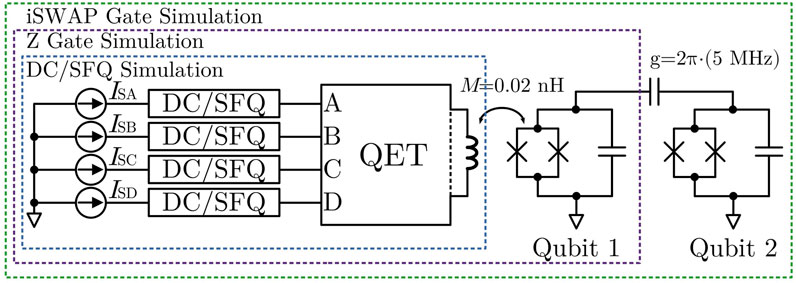
FIGURE 4. Circuits for all simulations.

FIGURE 5

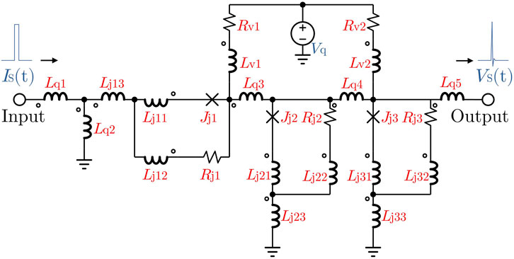
FIGURE 5. Simulation circuits of DC/SFQ.

FIGURE 6

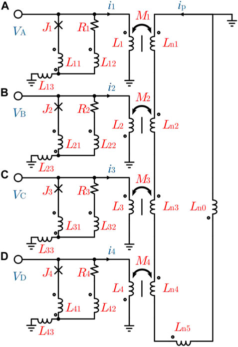
FIGURE 6. Simulation circuits of QET.

TABLE 1

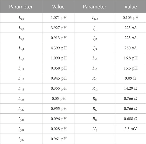
TABLE 1. Parameters of elements in the DC/SFQ.

TABLE 2

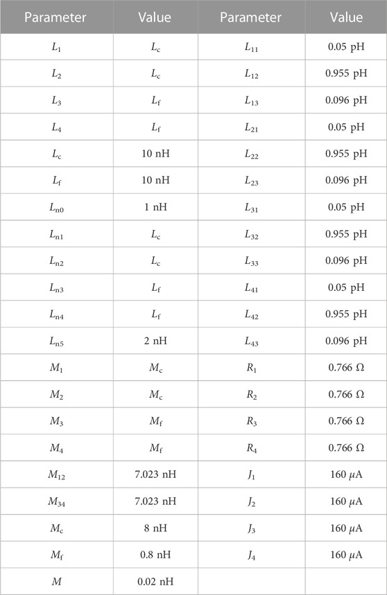
TABLE 2. Parameters of elements in the QET.

FIGURE 7

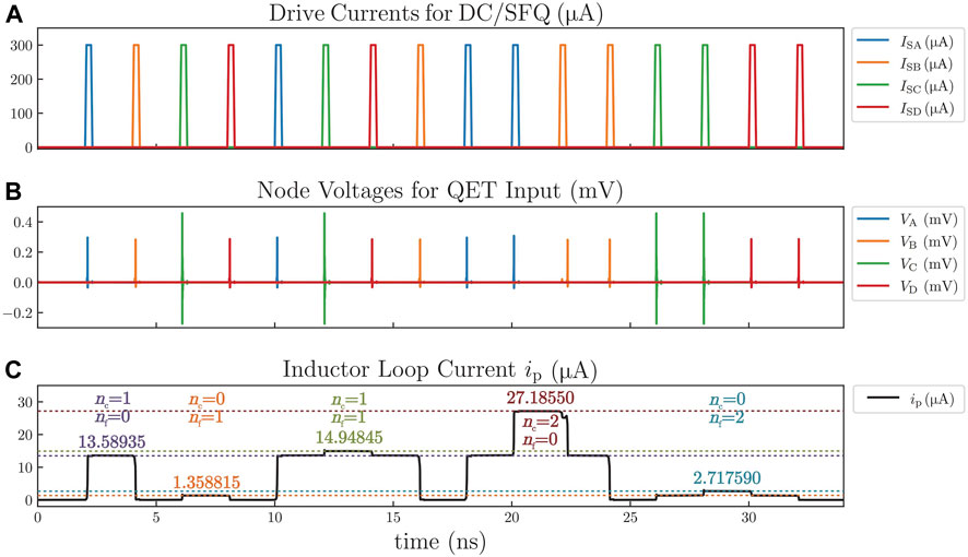
FIGURE 7. Time-domain responses of QET to SFQ pulses produced by DC/SFQ. (A) Drive currents for DC/SFQ, including I_SA, I_SB, I_SC, and I_SD. (B) Node voltages for QET input, including V_A, V_B, V_C, and V_D. (C) Inductor loop current i_p.

To change the inductor loop current i_p(t), which provides external flux Φ_e = Mi_p(t), n_c and n_f can be set by the SFQ pulse sequence from DC/SFQ. The simulation and analytical values of the inductor loop current with different n_c and n_f are compared in Table 3. First, by setting n_c = 1 and n_f = 0 with SFQ pulses sent to ports A and B (coarse tuning), Δi_pc can be extracted from the height of the leftmost lug boss of the inductor loop current curve in Figure 7C. The extraction value of Δi_pc is 13.58935 μA, which is close to the value 13.03599 μA, calculated by Eq. 37 with a relative deviation of 4.245%. Similarly, by setting n_c = 0 and n_f = 1 with SFQ pulses sent to ports C and D (fine-tuning), Δi_pf can also be extracted as 1.358815 μA from the second left current lug boss, which is also close to analytical solution 1.303599 μA from Eq. 37 with relative deviation 4.236%. Therefore, r_cf from this simulation is 10.00088 according to Eq. 48, almost the same as 10.0, the theory value from analytical solutions.

TABLE 3

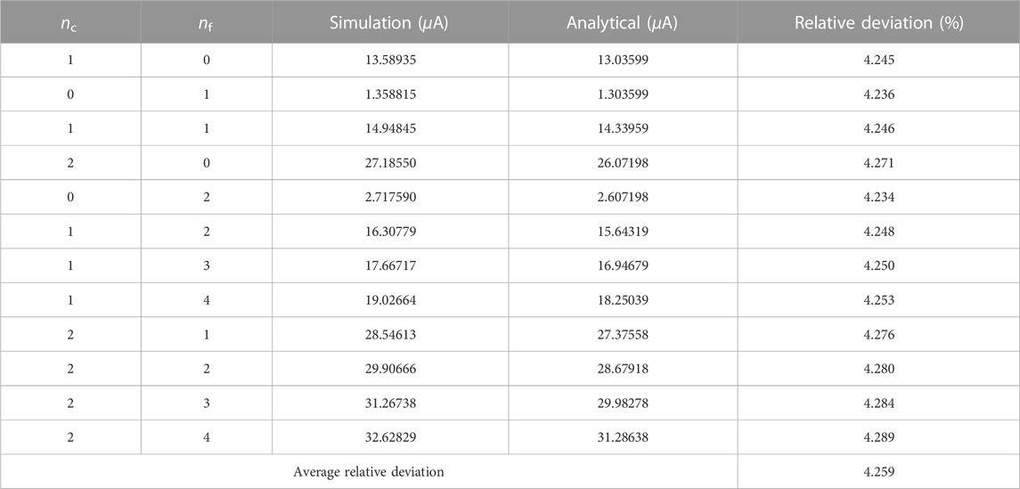
TABLE 3. Simulation and analytical values of the inductor loop current i_p with different n_c and n_f in the simulation for a single QET.

By setting n_c = 1 and n_f = 1, the two parts of the inductor loop current correspondingly made by coarse tuning and fine-tuning can be accumulated, as shown in the third left lug boss in Figure 7C. By setting n_c = 2 and n_f = 0, the inductor loop current can be double times Δi_pc. Similarly, by setting n_c = 0 and n_f = 2, the inductor loop current can also be double times Δi_pf. Generally, if the inductor loop current is required to be N_c times Δi_pc plus N_f times Δi_pf, then n_c should be set as N_c and n_f should be set as N_f according to Eq 41. The relative deviations between analytical solutions and simulation solutions of i_p for other cases (n_c = 1 when n_f = 2, 3, 4 and n_c = 2 when n_f = 1, 2, 3, 4) are also calculated, and the average relative deviation is 4.259%, as shown in Table 3.

The waveform of the inductor loop current is similar to composited square waves on the whole. Their rising and falling edges are steep, which helps avoid crosstalk when the qubit frequency is changing across frequencies of other qubits or resonators because the qubit frequency is changed quickly enough within time (several picoseconds) much shorter than a gate operation time (several nanoseconds).

4.2 Z Gate by a QET

The simulation in this subsection shows how a QET can perform a Z gate. The circuit for simulation is defined as the circuit in the purple-dashed-line box of Figure 4, which is based on the circuit of the former simulation in the blue-dashed-line box. The controlled qubit, Qubit 1, is a symmetric flux-tunable transmon connected to the former circuit, so we set d = 0 and E_J1 = E_J2 = E_J. Qubit 2 is ignored temporarily. By controlling the time interval of two SFQ pulses inputted to ports A and B of the QET, the phase of a flux-tunable transmon can be adjusted. Qubit 1 is driven only by coarse tuning with n_c = 1, so we set i_i = 0 and i_w = Δi_pc. Then, Δω(t) can be approximately treated as the constant Δω_q when t_s⩽t⩽t_e; that is,

$i_{\text{z}}\left(t\right)=i_{\text{p}}\left(t\right)=\left\{\begin{array}{cc}\mathrm{\Delta }{i}_{\text{pc}},\hfill & t_{\text{s}}⩽t⩽t_{\text{e}},\hfill \\ 0,\hfill & 0⩽t<t_{\text{s}}\mathrm{o}\mathrm{r}t>t_{\text{e}},\hfill \end{array}\right.(88)$

and

$\mathrm{\Delta }{\omega }_{\text{q}}=\frac{4\sqrt{E_{\text{C}}{E}_{\text{J}}}}{\hslash }\left(\sqrt{\left|\cos \left(\pi \frac{M\mathrm{\Delta }{i}_{\text{pc}}}{{\mathrm{\Phi }}_0}\right)\right|}-1\right).(89)$

Then, with Eqs 86, 89, we have

$\phi =\frac{4\sqrt{E_{\text{C}}{E}_{\text{J}}}}{\hslash }\left(1-\sqrt{\left|\cos \left(\pi \frac{M\mathrm{\Delta }{i}_{\text{pc}}}{{\mathrm{\Phi }}_0}\right)\right|}\right)t_{\text{z}}.(90)$

The evolution operator ${\tilde{U}}_{\text{dz}}$ becomes

$\begin{array}{cc}\hfill & {\tilde{U}}_{\text{dz}}=\hfill \\ \hfill & \left(\begin{array}{cc}\hfill 1\hfill & \hfill 0\hfill \\ \hfill 0\hfill & \hfill \exp \left(\mathrm{i}\frac{4\sqrt{E_{\text{C}}{E}_{\text{J}}}}{\hslash }\left(1-\sqrt{\left|\cos \left(\pi \frac{M\mathrm{\Delta }{i}_{\text{pc}}}{{\mathrm{\Phi }}_0}\right)\right|}\right)t_{\text{z}}\right)\hfill \end{array}\right).\hfill \end{array}(91)$

By designing the qubit and QET, the parameters E_C, E_J, M, and Δi_pc can be determined properly to make t_z in a range easy to realize. Then, for more precise control, the value of t_z should be optimized in practical experiments. Fine-tuning can also be performed to compensate for gate errors. In this simulation as a simple case, there are E_J/ℏ = 2π ⋅ (11.147 GHz), E_C/ℏ = 2π ⋅ (148.628 MHz), M = 0.02 nH, and Δi_pc = 13.58935 μA. Moreover, to realize a Z gate, t_z should be 2.261 ns by solving the equation φ = π with Eq 90. The initial state of Qubit 1 is set as

$|\psi {\rangle }_{\text{init}}=\frac{1}{\sqrt{2}}|0\rangle +\frac{1}{\sqrt{2}}|1\rangle .(92)$

The data on i_p(t) are first extracted from its time-domain simulation in WRSpice, similar to the former simulation of a single QET without the qubit. Then, it is imported into the Z gate simulation program using QuTip [22,23] to calculate the time-domain data on the drive Hamiltonian for Z control. By calling the function solving master equation or Schrödinger equation of QuTip, like qutip.mesolve() or qutip.sesolve(), the time evolution of the qubit state changed by a Z gate operated by the QET can be figured out with a total Hamiltonian H consisting of drive Hamiltonian H_dz and idle qubit Hamiltonian H₀, which is expressed by Eqs 75–78. The anharmonicity of the qubit is also considered in the simulation. Therefore, the creation operator a^† and annihilation operator a are treated as 3 × 3 matrices, and the state vectors are all 3-dimensional. The state vectors in the simulation results are projected onto the computational basis to obtain the qubit states in the 2-dimension computational space.

The simulation results for a Z gate by the QET in the rotating frame are presented in Figure 8. In addition to the waveforms, including (A) drive currents for DC/SFQ, (B) node voltages for the QET input, and (C) inductor loop current, (D) the frequencies of the qubit eigenenergies and (E) the qubit frequency are also plotted in Figure 8. The black trajectory of the point representing the qubit state on the surface of the Bloch sphere is drawn in Figure 9. In this simulation, the gate operation time of 2.261 ns is actually controlled by setting the time interval of the rising edges of two square-wave pulses in Figure 8A. During the period of gate operation (in the lug boss of the inductor loop current curve), the qubit frequency is kept at 4.779 GHz with E_JS/E_C = 137.5, changed from 5.0 GHz with E_JS/E_C = 150. The end state of the qubit becomes

$|\psi {\rangle }_{\text{end}}=0.70943|0\rangle +\left(-0.70476-0.0049432\mathrm{i}\right)|1\rangle ,(93)$

which is close to the ideal end state

$|\psi {\rangle }_{\text{iend}}=\frac{1}{\sqrt{2}}|0\rangle -\frac{1}{\sqrt{2}}|1\rangle .(94)$

The Z gate fidelity for only this time of operation is ${\mathcal{F}}_{\text{Z}}=99.99884\%$.

FIGURE 8

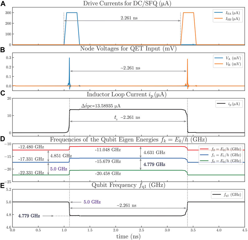
FIGURE 8. Z gate time-domain simulation results. (A) Drive currents for DC/SFQ, including I_SA, I_SB, I_SC, and I_SD. (B) Node voltages for QET input, including V_A, V_B, V_C, and V_D. (C) Inductor loop current i_p. (D) Frequencies of the qubit eigenenergies f_k. (E) Qubit frequency f_q1.

FIGURE 9

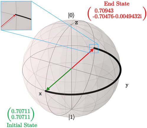
FIGURE 9. Trajectory of the point representing qubit state in Z gate simulation (in black).

If relaxation and dephasing are considered, then the simulation should obey the master equation describing the time evolution of a transmon coupled to the environment [24]:

$\dot{\rho }=-\frac{\mathrm{i}}{\hslash }\left[H,\rho \right]+\gamma \mathcal{D}\left[a\right]\rho +2{\gamma }_{\phi }\mathcal{D}\left[a^{†}a\right]\rho ,(95)$

where γ is the relaxation rate and γ_φ is the pure dephasing rate. H is the Hamiltonian described by Eq 75. ρ is the density matrix of the qubit. With approximation [24,25], the relationships of the two rates, T₁ and T₂, are

$\gamma \approx \frac{1}{T_1},(96)$

${\gamma }_{\phi }=\frac{1}{T_2}-\frac{1}{2T_1}.(97)$

For transmon based on Al/AlOx/Al Josephson junctions, the typical range of T₁ is 10 ∼ 110 μs, and the typical range of T₂ is 2 ∼ 18 µs [26–28]. In the simulation, T₁ is set as 50 µs, and T₂ is set as 10 μs. The density matrix of the initial state is

${\rho }_{\text{init}}=|\psi {\rangle }_{\text{init}}\langle \psi {|}_{\text{init}}=\left[\begin{array}{ccc}\hfill 0.5\hfill & \hfill 0.5\hfill & \hfill 0\hfill \\ \hfill 0.5\hfill & \hfill 0.5\hfill & \hfill 0\hfill \\ \hfill 0\hfill & \hfill 0\hfill & \hfill 0\hfill \end{array}\right].(98)$

The simulation results for a Z gate with relaxation and dephasing show that the density matrix of the end state is

${\rho }_{\text{end}}=\left[\begin{array}{ccc}\hfill 0.50004\hfill & \hfill -0.49977+0.0031974\mathrm{i}\hfill & \hfill 0\hfill \\ \hfill -0.49977-0.0031974\mathrm{i}\hfill & \hfill 0.49996\hfill & \hfill 0\hfill \\ \hfill 0\hfill & \hfill 0\hfill & \hfill 0\hfill \end{array}\right].(99)$

Additionally, the density matrix of the ideal end state is

${\rho }_{\text{iend}}=\left[\begin{array}{ccc}\hfill 0.5\hfill & \hfill -0.5\hfill & \hfill 0\hfill \\ \hfill -0.5\hfill & \hfill 0.5\hfill & \hfill 0\hfill \\ \hfill 0\hfill & \hfill 0\hfill & \hfill 0\hfill \end{array}\right].(100)$

Therefore, the fidelity of the Z gate with relaxation and dephasing for only this time is ${\mathcal{F}}_{\text{Z}}^{\prime }=99.98832\%$, which is smaller than ${\mathcal{F}}_{\text{Z}}=99.99884\%$.

4.3 iSWAP Gate by a QET

The simulation in this subsection shows how a QET can perform an iSWAP gate by making the frequency of Qubit 1 the same as that of Qubit 2. The corresponding Hamiltonian (considering rotating wave approximation (RWA) [20]) is

$H=\hslash (\mathrm{\Delta }\omega a_1^{†}{a}_1+{\omega }_{\text{q}1}{a}_1^{†}{a}_1+\frac{\alpha }{2}{a}_1^{†}{a}_1^{†}{a}_1{a}_1+{\omega }_{\text{q}2}{a}_2^{†}{a}_2+\frac{\alpha }{2}{a}_2^{†}{a}_2^{†}{a}_2{a}_2+g\left(a_1^{†}{a}_2+a_1{a}_2^{†}\right)).(101)$

Here, the two qubits have the same anharmonicity α but different idle frequencies ω_q1 and ω_q2. The creation and annihilation operators are defined as follows:

$a_1^{†}=a^{†}\otimes I,(102)$

$a_1=a\otimes I,(103)$

$a_2^{†}=I\otimes a^{†},(104)$

$a_2=I\otimes a,(105)$

where Δω is the frequency variation of Qubit 1 caused by the QET. I is a 3 × 3 identity matrix. As defined in the last Section 4.2, a^† and a are 3 × 3 matrices as the creation operator and the annihilation operator for a single qubit, respectively. Therefore, the state vectors of qubits in the iSWAP gate simulations are 9-dimensional, and their density matrices are 9 × 9 matrices. Compared with the former simulation for the Z gate, the method of this simulation with WRSpice and QuTip remains unchanged, but the simulation circuit is enlarged, as shown in the green-dashed-line box in Figure 4. The coupling strength between Qubit 1 and Qubit 2 is g = 2π ⋅ (5 MHz). The results are presented in Figure 10. Figure 10A shows the drive currents for DC/SFQ, including I_SA and I_SB. Figure 10B presents the node voltages for the QET input, including V_A and V_B. Figure 10C shows the curve of the inductor loop current i_p. Figure 10D shows the curve of frequencies of Qubit 1 and Qubit 2 (f_q1 and f_q2). Figure 10E shows the probability of the qubit state |ψ⟩ populating on |01⟩ or |10⟩.

FIGURE 10

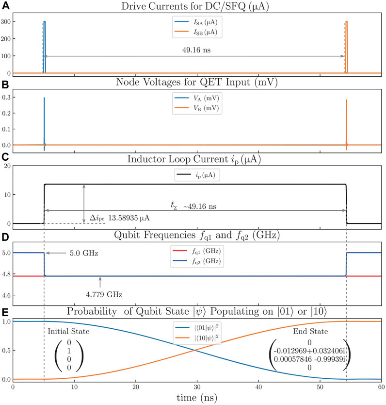
FIGURE 10. iSWAP gate time-domain simulation results. (A) Drive currents for DC/SFQ, including I_SA and I_SB. (B) Node voltage for QET input. (C) Inductor loop current. (D) Qubit frequencies. (E) Probability of the qubit state |ψ⟩ populating on |01⟩ or |10⟩.

The frequency of Qubit 1 (5.0 GHz) is tuned to the same level as the frequency of Qubit 2 (4.779 GHz) with i_p = Δi_pc = 13.58935 μA by inputting an SFQ pulse to port A of the QET. Then, the QET does nothing for t_z = 49.16 ns to wait for state swapping between Qubit 1 and Qubit 2 with the initial state:

$|\psi {\rangle }_{\text{init}}=|01\rangle .(106)$

When they finish swapping the qubit state, the second SFQ pulse is inputted to port B of the QET, which makes Qubit 1 back to its idle frequency. With the ideal end state,

$|\psi {\rangle }_{\text{iend}}=-\mathrm{i}|10\rangle (107)$

and the actual end state

$|\psi {\rangle }_{\text{end}}=\left(-0.012969+0.032406\mathrm{i}\right)|01\rangle +\left(0.00057846-0.99939\mathrm{i}\right)|10\rangle (108)$

in the simulation, the fidelity of the iSWAP gate (49.16 ns) for only this time of operation is ${\mathcal{F}}_{\text{iSWAP}}=99.93906\%$.

Usually, for two qubits coupling with g = 2π ⋅ (5 MHz), the iSWAP gate needs 50 ns. However, here the gate operation time is optimized as 49.16 ns to eliminate the extra phase shift of Qubit 1 caused by changing its frequency and to ensure that the fidelity of the iSWAP gate is high enough at the same time. The optimal gate operation time can be found by performing the simulation with the same other parameters but different values of gate operation time around 50 ns. As shown in Figure 11, the point at 49.16 ns has almost 0 extra phase shift (0.00058 rad) with a high enough fidelity of 99.93906%, which is a little smaller than the maximum value of 99.95724% at 50.35 ns.

FIGURE 11

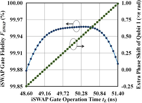
FIGURE 11. Fidelity ${\mathcal{F}}_{\text{iSWAP}}$ of the iSWAP gate and the extra phase shift of Qubit 1 with different gate operation time t_Z.

Similar to the simulation of the Z gate in the last Section 4.2, the simulation of the iSWAP gate considering the relaxation and dephasing is also performed. For the two-qubit system in the simulation, assuming that both qubits have the same relaxation time T₁ and dephasing time T₂, the master equation is

$\dot{\rho }=-\frac{\mathrm{i}}{\hslash }\left[H,\rho \right]+\gamma \mathcal{D}\left[a_1\right]\rho +2{\gamma }_{\phi }\mathcal{D}\left[a_1^{†}{a}_1\right]\rho +\gamma \mathcal{D}\left[a_2\right]\rho +2{\gamma }_{\phi }\mathcal{D}\left[a_2^{†}{a}_2\right]\rho ,(109)$

where H is the Hamiltonian described by Eq 101. ρ is the 9 × 9 density matrix of the two-qubit system. With the initial state,

$|\psi {\rangle }_{\text{init}}=|01\rangle =\left[\begin{array}{c}\hfill 1\hfill \\ \hfill 0\hfill \\ \hfill 0\hfill \end{array}\right]\otimes \left[\begin{array}{c}\hfill 0\hfill \\ \hfill 1\hfill \\ \hfill 0\hfill \end{array}\right]=\left[\begin{array}{c}\hfill 0\hfill \\ \hfill 1\hfill \\ \hfill 0\hfill \\ \hfill 0\hfill \\ \hfill 0\hfill \\ \hfill 0\hfill \\ \hfill 0\hfill \\ \hfill 0\hfill \\ \hfill 0\hfill \end{array}\right],(110)$

the density matrix of the initial state is

${\rho }_{\text{init}}=|\psi {\rangle }_{\text{init}}\langle \psi {|}_{\text{init}}=\left[\begin{array}{ccccccccc}\hfill 0\hfill & \hfill 0\hfill & \hfill 0\hfill & \hfill 0\hfill & \hfill 0\hfill & \hfill 0\hfill & \hfill 0\hfill & \hfill 0\hfill & \hfill 0\hfill \\ \hfill 0\hfill & \hfill 1\hfill & \hfill 0\hfill & \hfill 0\hfill & \hfill 0\hfill & \hfill 0\hfill & \hfill 0\hfill & \hfill 0\hfill & \hfill 0\hfill \\ \hfill 0\hfill & \hfill 0\hfill & \hfill 0\hfill & \hfill 0\hfill & \hfill 0\hfill & \hfill 0\hfill & \hfill 0\hfill & \hfill 0\hfill & \hfill 0\hfill \\ \hfill 0\hfill & \hfill 0\hfill & \hfill 0\hfill & \hfill 0\hfill & \hfill 0\hfill & \hfill 0\hfill & \hfill 0\hfill & \hfill 0\hfill & \hfill 0\hfill \\ \hfill 0\hfill & \hfill 0\hfill & \hfill 0\hfill & \hfill 0\hfill & \hfill 0\hfill & \hfill 0\hfill & \hfill 0\hfill & \hfill 0\hfill & \hfill 0\hfill \\ \hfill 0\hfill & \hfill 0\hfill & \hfill 0\hfill & \hfill 0\hfill & \hfill 0\hfill & \hfill 0\hfill & \hfill 0\hfill & \hfill 0\hfill & \hfill 0\hfill \\ \hfill 0\hfill & \hfill 0\hfill & \hfill 0\hfill & \hfill 0\hfill & \hfill 0\hfill & \hfill 0\hfill & \hfill 0\hfill & \hfill 0\hfill & \hfill 0\hfill \\ \hfill 0\hfill & \hfill 0\hfill & \hfill 0\hfill & \hfill 0\hfill & \hfill 0\hfill & \hfill 0\hfill & \hfill 0\hfill & \hfill 0\hfill & \hfill 0\hfill \\ \hfill 0\hfill & \hfill 0\hfill & \hfill 0\hfill & \hfill 0\hfill & \hfill 0\hfill & \hfill 0\hfill & \hfill 0\hfill & \hfill 0\hfill & \hfill 0\hfill \end{array}\right].(111)$

Moreover, the density matrix of the end state is

${\rho }_{\text{end}}=\left[\begin{array}{ccccccccc}\hfill 0.0011993\hfill & \hfill 0\hfill & \hfill 0\hfill & \hfill 0\hfill & \hfill 0\hfill & \hfill 0\hfill & \hfill 0\hfill & \hfill 0\hfill & \hfill 0\hfill \\ \hfill 0\hfill & \hfill 0.00242833\hfill & \hfill 0\hfill & \hfill -0.0062854+0.011886\mathrm{i}\hfill & \hfill 0\hfill & \hfill 0\hfill & \hfill 0\hfill & \hfill 0\hfill & \hfill 0\hfill \\ \hfill 0\hfill & \hfill 0\hfill & \hfill 0\hfill & \hfill 0\hfill & \hfill 0\hfill & \hfill 0\hfill & \hfill 0\hfill & \hfill 0\hfill & \hfill 0\hfill \\ \hfill 0\hfill & \hfill -0.0062854-0.011886\mathrm{i}\hfill & \hfill 0\hfill & \hfill 0\hfill & \hfill 0\hfill & \hfill 0\hfill & \hfill 0\hfill & \hfill 0\hfill & \hfill 0\hfill \\ \hfill 0\hfill & \hfill 0\hfill & \hfill 0\hfill & \hfill 0\hfill & \hfill 0.996373\hfill & \hfill 0\hfill & \hfill 0\hfill & \hfill 0\hfill & \hfill 0\hfill \\ \hfill 0\hfill & \hfill 0\hfill & \hfill 0\hfill & \hfill 0\hfill & \hfill 0\hfill & \hfill 0\hfill & \hfill 0\hfill & \hfill 0\hfill & \hfill 0\hfill \\ \hfill 0\hfill & \hfill 0\hfill & \hfill 0\hfill & \hfill 0\hfill & \hfill 0\hfill & \hfill 0\hfill & \hfill 0\hfill & \hfill 0\hfill & \hfill 0\hfill \\ \hfill 0\hfill & \hfill 0\hfill & \hfill 0\hfill & \hfill 0\hfill & \hfill 0\hfill & \hfill 0\hfill & \hfill 0\hfill & \hfill 0\hfill & \hfill 0\hfill \\ \hfill 0\hfill & \hfill 0\hfill & \hfill 0\hfill & \hfill 0\hfill & \hfill 0\hfill & \hfill 0\hfill & \hfill 0\hfill & \hfill 0\hfill & \hfill 0\hfill \end{array}\right].(112)$

The density matrix of the ideal end state is

${\rho }_{\text{iend}}=\left[\begin{array}{ccccccccc}\hfill 0\hfill & \hfill 0\hfill & \hfill 0\hfill & \hfill 0\hfill & \hfill 0\hfill & \hfill 0\hfill & \hfill 0\hfill & \hfill 0\hfill & \hfill 0\hfill \\ \hfill 0\hfill & \hfill 0\hfill & \hfill 0\hfill & \hfill 0\hfill & \hfill 0\hfill & \hfill 0\hfill & \hfill 0\hfill & \hfill 0\hfill & \hfill 0\hfill \\ \hfill 0\hfill & \hfill 0\hfill & \hfill 0\hfill & \hfill 0\hfill & \hfill 0\hfill & \hfill 0\hfill & \hfill 0\hfill & \hfill 0\hfill & \hfill 0\hfill \\ \hfill 0\hfill & \hfill 0\hfill & \hfill 0\hfill & \hfill 1\hfill & \hfill 0\hfill & \hfill 0\hfill & \hfill 0\hfill & \hfill 0\hfill & \hfill 0\hfill \\ \hfill 0\hfill & \hfill 0\hfill & \hfill 0\hfill & \hfill 0\hfill & \hfill 0\hfill & \hfill 0\hfill & \hfill 0\hfill & \hfill 0\hfill & \hfill 0\hfill \\ \hfill 0\hfill & \hfill 0\hfill & \hfill 0\hfill & \hfill 0\hfill & \hfill 0\hfill & \hfill 0\hfill & \hfill 0\hfill & \hfill 0\hfill & \hfill 0\hfill \\ \hfill 0\hfill & \hfill 0\hfill & \hfill 0\hfill & \hfill 0\hfill & \hfill 0\hfill & \hfill 0\hfill & \hfill 0\hfill & \hfill 0\hfill & \hfill 0\hfill \\ \hfill 0\hfill & \hfill 0\hfill & \hfill 0\hfill & \hfill 0\hfill & \hfill 0\hfill & \hfill 0\hfill & \hfill 0\hfill & \hfill 0\hfill & \hfill 0\hfill \\ \hfill 0\hfill & \hfill 0\hfill & \hfill 0\hfill & \hfill 0\hfill & \hfill 0\hfill & \hfill 0\hfill & \hfill 0\hfill & \hfill 0\hfill & \hfill 0\hfill \end{array}\right].(113)$

The fidelity of the iSWAP gate by QET considering relaxation and dephasing is ${\mathcal{F}}_{\text{Z}}^{\prime }=99.81846\%$, which is a little worse than ${\mathcal{F}}_{\text{iSWAP}}=99.93906\%$.

5 Summary and outlook

In conclusion, we have proposed the QET device with the description of its circuit structure and theory for its SFQ-based digital Z control to a flux-tunable transmon. A QET can convert SFQ pulses to external flux for qubits. Therefore, it can set the idle frequency of a flux-tunable transmon and, at the same time, perform gate operations involving Z control, such as Z gates and iSWAP gates, thus paving an approach for digital Z control of an SFQ-based quantum-classical interface, which is highly desirable for the research and development of a large-scale superconducting quantum computer.

For integrating with flux-tunable transmons and avoiding noise from SFQ circuits simultaneously, the parts of QETs consisting of flux bias units can be fabricated on another substrate, which is electrically connected to the qubit chip with through silicon vias (TSVs) and indium bumps of a silicon interposer [15,16]. In order to realize mutual inductances between transmon SQUIDs and inductor loops of QETs, TSVs and indium bumps should be parts of inductor loops so that the piece of the inductor line of an inductor loop for flux bias can be fabricated on the qubit chip or the surface of the silicon interposer faced to qubits. To eliminate the electrical loss of inductor loops, the material of TSVs should be superconductive (e.g., TiN). QETs may also be used in other application scenarios requiring flux tuning, such as CZ gates [29], flux-tunable couplers [30,31], and qubit readout with a Josephson photomultiplier [32]. Further research should design and fabricate this device for experiments about SFQ-based digital control of qubits, especially flux-tunable transmons.

Data availability statement

The original contributions presented in the study are included in the article/supplementary material. Further inquiries can be directed to the corresponding author.

Author contributions

Conceptualization, formula derivation, simulation, and writing: XG; formula derivation, revision: KH; validation and investigation: RH; review and editing: JL; resources: WC. All authors contributed to the article and approved the submitted version.

Funding

This work was partially supported by the key R&D program of Guangdong province (grant no. 2019B010143002).

Acknowledgments

XG acknowledges the discussion with Yongcheng He, Genting Dai, Liangliang Yang, Xinyu Wu, Qing Yu, Mingjun Cheng, and Guodong Chen about the methodology of the article.

Conflict of interest

The authors declare that the research was conducted in the absence of any commercial or financial relationships that could be construed as a potential conflict of interest.

Publisher’s note

All claims expressed in this article are solely those of the authors and do not necessarily represent those of their affiliated organizations or those of the publisher, the editors, and the reviewers. Any product that may be evaluated in this article, or claim that may be made by its manufacturer, is not guaranteed or endorsed by the publisher.

References

1. Barends R, Kelly J, Megrant A, Veitia A, Sank D, Jeffrey E, et al. Superconducting quantum circuits at the surface code threshold for fault tolerance. Nature (2014) 508:500–3. doi:10.1038/nature13171

PubMed Abstract | CrossRef Full Text | Google Scholar

2. Arute F, Arya K, Babbush R, Bacon D, Bardin JC, Barends R, et al. Quantum supremacy using a programmable superconducting processor. Nature (2019) 574:505–10. doi:10.1038/s41586-019-1666-5

PubMed Abstract | CrossRef Full Text | Google Scholar

3. Likharev K, Semenov V. Rsfq logic/memory family: A new josephson-junction technology for sub-terahertz-clock-frequency digital systems. IEEE Trans Appl Superconductivity (1991) 1:3–28. doi:10.1109/77.80745

CrossRef Full Text | Google Scholar

4. McDermott R, Vavilov M, Plourde B, Wilhelm F, Liebermann P, Mukhanov O, et al. Quantum–classical interface based on single flux quantum digital logic. Quan Sci Technol (2018) 3:024004. doi:10.1088/2058-9565/aaa3a0

CrossRef Full Text | Google Scholar

5. McDermott R, Vavilov M. Accurate qubit control with single flux quantum pulses. Phys Rev Appl (2014) 2:014007. doi:10.1103/physrevapplied.2.014007

CrossRef Full Text | Google Scholar

6. Leonard E, Beck MA, Nelson J, Christensen BG, Thorbeck T, Howington C, et al. Digital coherent control of a superconducting qubit. Phys Rev Appl (2019) 11:014009. doi:10.1103/physrevapplied.11.014009

CrossRef Full Text | Google Scholar

7. Liebermann PJ, Wilhelm FK. Optimal qubit control using single-flux quantum pulses. Phys Rev Appl (2016) 6:024022. doi:10.1103/physrevapplied.6.024022

CrossRef Full Text | Google Scholar

8. Li K, McDermott R, Vavilov MG. Hardware-efficient qubit control with single-flux-quantum pulse sequences. Phys Rev Appl (2019) 12:014044. doi:10.1103/physrevapplied.12.014044

CrossRef Full Text | Google Scholar

9. Vozhakov V, Bastrakova MV, Klenov NV, Satanin A, Soloviev II. Speeding up qubit control with bipolar single-flux-quantum pulse sequences. Quan Sci Technol (2023) 8:035024. doi:10.1088/2058-9565/acd9e6

CrossRef Full Text | Google Scholar

10. Jokar MR, Rines R, Pasandi G, Cong H, Holmes A, Shi Y, et al. Digiq: A scalable digital controller for quantum computers using sfq logic. In: Proceedings of the 2022 IEEE International Symposium on High-Performance Computer Architecture (HPCA); April 2022; Seoul, Korea (2022). p. 400–14. doi:10.1109/HPCA53966.2022.00037

CrossRef Full Text | Google Scholar

11. Dalgaard M, Motzoi F, Sørensen JJ, Sherson J. Global optimization of quantum dynamics with alphazero deep exploration. npj Quan Inf (2020) 6:6–9. doi:10.1038/s41534-019-0241-0

CrossRef Full Text | Google Scholar

12. Jokar MR, Rines R, Chong FT. Practical implications of sfq-based two-qubit gates. In: Proceedings of the 2021 IEEE International Conference on Quantum Computing and Engineering (QCE); October 2021; Broomfield, CO, USA (2021). p. 402–12. doi:10.1109/QCE52317.2021.00061

CrossRef Full Text | Google Scholar

13. Wang Y, Gao W, Liu K, Ji B, Wang Z, Lin Z. Single-flux-quantum-activated controlled-z gate for transmon qubits. Phys Rev Appl (2023) 19:044031. doi:10.1103/physrevapplied.19.044031

CrossRef Full Text | Google Scholar

14. Johnson M, Bunyk P, Maibaum F, Tolkacheva E, Berkley A, Chapple E, et al. A scalable control system for a superconducting adiabatic quantum optimization processor. Superconductor Sci Technol (2010) 23:065004. doi:10.1088/0953-2048/23/6/065004

CrossRef Full Text | Google Scholar

15. Rosenberg D, Kim D, Das R, Yost D, Gustavsson S, Hover D, et al. 3d integrated superconducting qubits. npj Quan Inf (2017) 3:42–5. doi:10.1038/s41534-017-0044-0

CrossRef Full Text | Google Scholar

16. Rosenberg D, Weber SJ, Conway D, Yost D-RW, Mallek J, Calusine G, et al. Solid-state qubits: 3d integration and packaging. IEEE Microwave Mag (2020) 21:72–85. doi:10.1109/mmm.2020.2993478

CrossRef Full Text | Google Scholar

17. Bunyk PI, Hoskinson EM, Johnson MW, Tolkacheva E, Altomare F, Berkley AJ, et al. Architectural considerations in the design of a superconducting quantum annealing processor. IEEE Trans Appl Superconductivity (2014) 24:1–10. doi:10.1109/tasc.2014.2318294

CrossRef Full Text | Google Scholar

18. Narayana S, Semenov V. Energy dissipation minimization in superconducting circuits. In: AM Luiz, editor. Superconductivity. Rijeka: IntechOpen (2011). chap. 5. doi:10.5772/16285

CrossRef Full Text | Google Scholar

19. Koch J, Terri MY, Gambetta J, Houck AA, Schuster DI, Majer J, et al. Charge-insensitive qubit design derived from the cooper pair box. Phys Rev A (2007) 76:042319. doi:10.1103/physreva.76.042319

CrossRef Full Text | Google Scholar

20. Krantz P, Kjaergaard M, Yan F, Orlando TP, Gustavsson S, Oliver WD. A quantum engineer’s guide to superconducting qubits. Appl Phys Rev (2019) 6:021318. doi:10.1063/1.5089550

CrossRef Full Text | Google Scholar

21. Li G. Research on superconducting RSFQ circuit for qubit control. Ph.D. thesis. Tsinghua: Tsinghua University (2018).

Google Scholar

22. Johansson J, Nation P, Nori F. Qutip: An open-source python framework for the dynamics of open quantum systems. Comput Phys Commun (2012) 183:1760–72. doi:10.1016/j.cpc.2012.02.021

CrossRef Full Text | Google Scholar

23. Johansson J, Nation P, Nori F. Qutip 2: A python framework for the dynamics of open quantum systems. Comput Phys Commun (2013) 184:1234–40. doi:10.1016/j.cpc.2012.11.019

CrossRef Full Text | Google Scholar

24. Blais A, Grimsmo AL, Girvin SM, Wallraff A. Circuit quantum electrodynamics. Rev Mod Phys (2021) 93:025005. doi:10.1103/revmodphys.93.025005

CrossRef Full Text | Google Scholar

25. Schoelkopf R, Clerk A, Girvin S, Lehnert K, Devoret M. Qubits as spectrometers of quantum noise Quantum noise in mesoscopic physics (2003). Available at: https://arxiv.org/abs/cond-mat/0210247 (Accessed June 28, 2023).

Google Scholar

26. Xu S, Sun Z-Z, Wang K, Xiang L, Bao Z, Zhu Z, et al. Digital simulation of non-abelian anyons with 68 programmable superconducting qubits (2022). Available at: https://arxiv.org/abs/2211.09802 (Accessed June 29, 2023).

Google Scholar

27. Shi Y-H, Liu Y, Zhang Y-R, Xiang Z, Huang K, Liu T, et al. Observing topological zero modes on a 41-qubit superconducting processor (2022). Available at: https://arxiv.org/abs/2211.05341 (Accessed June 29, 2023).

Google Scholar

28. Wu Y, Bao W-S, Cao S, Chen F, Chen M-C, Chen X, et al. Strong quantum computational advantage using a superconducting quantum processor. Phys Rev Lett (2021) 127:180501. doi:10.1103/physrevlett.127.180501

PubMed Abstract | CrossRef Full Text | Google Scholar

29. Xu Y, Chu J, Yuan J, Qiu J, Zhou Y, Zhang L, et al. High-fidelity, high-scalability two-qubit gate scheme for superconducting qubits. Phys Rev Lett (2020) 125:240503. doi:10.1103/physrevlett.125.240503

PubMed Abstract | CrossRef Full Text | Google Scholar

30. Chen Y, Neill C, Roushan P, Leung N, Fang M, Barends R, et al. Qubit architecture with high coherence and fast tunable coupling. Phys Rev Lett (2014) 113:220502. doi:10.1103/physrevlett.113.220502

PubMed Abstract | CrossRef Full Text | Google Scholar

31. Yan F, Krantz P, Sung Y, Kjaergaard M, Campbell DL, Orlando TP, et al. Tunable coupling scheme for implementing high-fidelity two-qubit gates. Phys Rev Appl (2018) 10:054062. doi:10.1103/physrevapplied.10.054062

CrossRef Full Text | Google Scholar

32. Opremcak A, Pechenezhskiy I, Howington C, Christensen B, Beck M, Leonard E, et al. Measurement of a superconducting qubit with a microwave photon counter. Science (2018) 361:1239–42. doi:10.1126/science.aat4625

PubMed Abstract | CrossRef Full Text | Google Scholar