Surveying an energy landscape

1 Introduction

Central to statistical physics are the canonical ensemble, its partition function, and as defining quantity the temperature on the one hand as well as the microcanonical ensemble and the density of states defined by energy on the other. While the energy in the canonical ensemble takes the form of a weighted average over all microstates, the temperature in the microcanonical ensemble becomes the inverse of the derivative of the logarithmic density of states. However, in 1997 Rugh [1] showed that it too can be expressed as an average of an observable comprising various derivatives of the Hamiltonian. The same formula had already been found by Gilat [2], but—judging by the number of citations—received very little attention. With Rugh’s work at hand, it was soon realized [3] that this relation among other things offers a way to verify the correctness of Monte Carlo (MC) computer simulations. Unfortunately, the formula involves a rather unwieldy term containing the Hamiltonian’s Hessian that is computationally demanding. In this study, we develop a formula that expresses the density of states of the system as a function of microcanonical averages of squared gradient and Laplacian of the Hamiltonian while avoiding this term.

In the last decades, MC simulations have become an important tool to investigate thermodynamic properties of models of complex systems. Today, many different techniques are used. In addition to the famous Metropolis algorithm [4] which samples from the canonical ensemble nowadays generalized ensemble methods have become more prevalent. Among these, flat-histogram methods such as multicanonical (MUCA) [5], the Wang-Landau method [6], and Statistical Temperature MC [7] aim to create the same ensemble where the distribution as a function of energy is constant. On the one hand, this allows one to reweight the data to a canonical ensemble with any desirable temperature, while on the other hand even if one is only interested in low-temperature behavior the inclusion of high energies allows the system to decorrelate more easily. To bias the system’s random walk such that this ensemble becomes the stationary distribution the logarithm of the density of states (DoS) or its derivative must be known with sufficient precision. This can be achieved in an iterative process [8,9] that analyses and incorporates successively created histograms or on the fly by permanently altering the estimate of the DoS [6] or its derivative [7] based only on the energy of the current state of the system. Either way, the estimate of the DoS that is created and employed to drive the algorithm is solely based on the energy time series. No other information is utilized.

It is an interesting exercise and test of the accuracy and precision achieved with our formula to measure the microcanonical properties of the energy landscape and use them to estimate the DoS during a flat-histogram MC simulation that at the same time is using that estimate to achieve a flat distribution in energy. In this study, we demonstrate this idea with two examples: A system of interacting Lennard-Jones particles and the O(n) vector spin model.

The paper is organized as follows: In Section 2 we once more derive the formula of Gilat and Rugh and proceed to calculate our alternative. In Section 3 we discuss how a flat-histogram algorithm can be formulated and develop a suitable method for numerical integration. We then apply the method to a Lennard-Jones system in Section 4 and to the O(n) vector spin model in Section 5. In Section 6 we finish with some concluding remarks.

2 Calculating the density of states

The DoS or partition sum of the microcanonical ensemble at energy E is given by

$g\left(E\right)=\int \delta \left(\mathcal{H}\left(\mathbf{X}\right)-E\right)\mathrm{d}{x}^N,(1)$

where $\mathcal{H}$ is the Hamiltonian of the system, N the number of degrees of freedom, and the integration goes over the entire state space. This can be rewritten as a surface integral

$g\left(E\right)={\int }_{A_E}\frac{1}{|\nabla \mathcal{H}\left(\mathbf{X}\right)|}\mathrm{d}{x}^{N-1},(2)$

with $A_E=\{\mathbf{X}:\mathcal{H}(\mathbf{X})=E\}$ being the surface of constant energy E and ∇ is the gradient ${(\frac{\mathrm{d}}{\mathrm{d}{x}_1},\frac{\mathrm{d}}{\mathrm{d}{x}_2},\dots ,\frac{\mathrm{d}}{\mathrm{d}{x}_N})}^T$. The microcanonical average of any observable Q(X) is given by

${⟨Q⟩}_E=\frac{1}{g\left(E\right)}\int \delta \left(\mathcal{H}\left(\mathbf{X}\right)-E\right)Q\left(\mathbf{X}\right)\mathrm{d}{x}^N(3)$

$=\frac{1}{g\left(E\right)}{\int }_{A_E}\frac{Q\left(\mathbf{X}\right)}{|\nabla \mathcal{H}\left(\mathbf{X}\right)|}\mathrm{d}{x}^{N-1}.(4)$

To be able to apply the divergence theorem we rewrite (2) again:

$g\left(E\right)={\int }_{A_E}\frac{\nabla \mathcal{H}\left(\mathbf{X}\right)}{{\left(\nabla \mathcal{H}\left(\mathbf{X}\right)\right)}^2}\cdot \mathbf{n}\left(\mathbf{X}\right)\mathrm{d}{x}^{N-1}.(5)$

Here, $\mathbf{n}=\nabla \mathcal{H}(\mathbf{X})/|\nabla \mathcal{H}(\mathbf{X})|$ is a unit vector perpendicular to the plane of constant energy and pointing to higher energies. It is therefore parallel to $\nabla \mathcal{H}(\mathbf{X})$. The derivative of the DoS with respect to energy is

$\frac{\mathrm{d}g\left(E\right)}{\mathrm{d}E}=\underset{\epsilon \to 0}{\lim }\frac{g\left(E+\epsilon \right)-g\left(E\right)}{\epsilon }.(6)$

We insert (5), apply the divergence theorem, and integrate perpendicular to the surfaces by multiplying the thickness of the integration volume $\frac{\epsilon }{|\nabla \mathcal{H}(\mathbf{X})|}$ and find

$\frac{\mathrm{d}g\left(E\right)}{\mathrm{d}E}={\int }_{A_E}\frac{1}{|\nabla \mathcal{H}\left(\mathbf{X}\right)|}\nabla \frac{\nabla \mathcal{H}\left(\mathbf{X}\right)}{{\left(\nabla \mathcal{H}\left(\mathbf{X}\right)\right)}^2}\mathrm{d}{x}^{N-1}.(7)$

Dividing by g(E) on both sides we obtain the known result [1,2,10–13]

$\frac{1}{g\left(E\right)}\frac{\mathrm{d}g\left(E\right)}{\mathrm{d}E}=\frac{\mathrm{d}\ln g\left(E\right)}{\mathrm{d}E}={⟨B\left(\mathbf{X}\right)⟩}_E(8)$

with

$\begin{array}{ll}\hfill B\left(\mathbf{X}\right)& =\nabla \frac{\nabla \mathcal{H}\left(\mathbf{X}\right)}{{\left(\nabla \mathcal{H}\left(\mathbf{X}\right)\right)}^2}\hfill \\ \hfill & =\frac{\mathrm{\Delta }\mathcal{H}\left(\mathbf{X}\right)}{{\left(\nabla \mathcal{H}\left(\mathbf{X}\right)\right)}^2}-2\frac{\nabla \mathcal{H}\left(\mathbf{X}\right)H\left(\mathbf{X}\right)\nabla \mathcal{H}\left(\mathbf{X}\right)}{{\left(\nabla \mathcal{H}\left(\mathbf{X}\right)\right)}^4},\hfill \end{array}(9)$

where $\mathrm{\Delta }={\sum }_{i=1}^N\frac{{\partial }^2}{\partial x_i^2}$ is the Laplace operator and H denotes the Hessian matrix of the Hamiltonian, $H_{ij}(\mathbf{X})=\frac{{\partial }^2\mathcal{H}(\mathbf{X})}{\partial x_i\partial x_j}$. The observable B which can in principle be calculated for any microstate X of the system at hand, allows us to determine the DoS up to a factor regardless of the applied algorithm:

$g\left(E\right)\propto \exp \left({\int }_{E_0}^E{⟨B⟩}_{E^{\prime }}\mathrm{d}{E}^{\prime }\right),(10)$

where E₀ can be chosen freely. It is worth noting that B relates directly to temperature. It is true by definition that its microcanonical average equals the inverse microcanonical temperature if the latter is defined as

${\left(T_{\text{micro}}{k}_{\mathrm{B}}\right)}^{-1}=\frac{\mathrm{d}{S}_{\text{micro}}}{\mathrm{d}E},S_{\text{micro}}=\ln g\left(E\right)(11)$

and it can easily be shown that its canonical average is equal to the inverse canonical temperature:

$\begin{array}{ll}\hfill \frac{\int B\left(\mathbf{X}\right)e^{-\beta E\left(\mathbf{X}\right)}\mathrm{d}{x}^N}{\int e^{-\beta E\left(\mathbf{X}\right)}\mathrm{d}{x}^N}& =\frac{\int {⟨B⟩}_{E^{\prime }}g\left(E^{\prime }\right)e^{-\beta E^{\prime }}\mathrm{d}{E}^{\prime }}{\int g\left(E^{\prime }\right)e^{-\beta E^{\prime }}\mathrm{d}{E}^{\prime }}\hfill \\ \hfill & =\frac{\int g^{\prime }\left(E^{\prime }\right)e^{-\beta E^{\prime }}\mathrm{d}{E}^{\prime }}{\int g\left(E^{\prime }\right)e^{-\beta E^{\prime }}\mathrm{d}{E}^{\prime }}\hfill \\ \hfill & =\beta ={\left(k_{\mathrm{B}}T\right)}^{-1}.\hfill \end{array}(12)$

While gradient and Laplace operator can be applied to $\mathcal{H}$ without too much computational effort¹ the determination of the Hessian matrix is very demanding and a simpler scheme would be preferable. We start again with the microcanonical average of some observable Q(X)

${⟨Q\left(\mathbf{X}\right)⟩}_E=\frac{1}{g\left(E\right)}{\int }_{A_E}\frac{Q\left(\mathbf{X}\right)}{|\nabla \mathcal{H}\left(\mathbf{X}\right)|}\mathrm{d}{x}^{N-1}(13)$

and now consider its energy derivative

$\begin{array}{ll}\hfill \frac{\mathrm{d}}{\mathrm{d}E}{\langle Q\left(\mathbf{X}\right)\rangle }_E& =\frac{\mathrm{d}}{\mathrm{d}E}\frac{{\int }_{A_E}\frac{Q\left(\mathbf{X}\right)}{|\nabla \mathcal{H}\left(\mathbf{X}\right)|}\mathrm{d}{x}^{n-1}}{g\left(E\right)}\hfill \\ \hfill & =\frac{\frac{\mathrm{d}}{\mathrm{d}E}{\int }_{A_E}\frac{Q\left(\mathbf{X}\right)}{|\nabla \mathcal{H}\left(\mathbf{X}\right)|}\mathrm{d}{x}^{n-1}}{g\left(E\right)}-{\langle Q\left(\mathbf{X}\right)\rangle }_E\frac{g^{\prime }\left(E\right)}{g\left(E\right)}.\hfill \end{array}(14)$

The integral can be transformed,

${\int }_{A_E}\frac{Q\left(\mathbf{X}\right)}{|\nabla \mathcal{H}\left(\mathbf{X}\right)|}\mathrm{d}{x}^{n-1}={\int }_{A_E}\frac{Q\left(\mathbf{X}\right)}{{\left(\nabla \mathcal{H}\left(\mathbf{X}\right)\right)}^2}\nabla \mathcal{H}\left(\mathbf{X}\right)\cdot \mathbf{n}\mathrm{d}{x}^{N-1},(15)$

and the derivative be calculated similarly to the procedure used above. Using differential quotient and divergence theorem we find

$\frac{\mathrm{d}}{\mathrm{d}E}{\int }_{A_E}\frac{Q\left(\mathbf{X}\right)}{|\nabla \mathcal{H}\left(\mathbf{X}\right)|}\mathrm{d}{x}^{n-1}={\int }_{A_E}\frac{\nabla \left(\frac{Q\left(\mathbf{X}\right)\nabla \mathcal{H}\left(\mathbf{X}\right)}{{\left(\nabla \mathcal{H}\left(\mathbf{X}\right)\right)}^2}\right)}{|\nabla \mathcal{H}\left(\mathbf{X}\right)|}\mathrm{d}{x}^{N-1}.(16)$

It follows that

$\frac{\mathrm{d}}{\mathrm{d}E}{⟨Q\left(\mathbf{X}\right)⟩}_E=\langle {\nabla \left(\frac{Q\left(\mathbf{X}\right)\nabla \mathcal{H}\left(\mathbf{X}\right)}{{\left(\nabla \mathcal{H}\left(\mathbf{X}\right)\right)}^2}\right)⟩}_E-{⟨Q\left(\mathbf{X}\right)⟩}_E\frac{\mathrm{d}\ln g\left(E\right)}{\mathrm{d}E}(17)$

and in particular by choosing $Q(\mathbf{X})={(\nabla \mathcal{H}(\mathbf{X}))}^2$ one obtains

$\frac{\mathrm{d}}{\mathrm{d}E}{⟨{\left(\nabla \mathcal{H}\left(\mathbf{X}\right)\right)}^2⟩}_E={⟨\mathrm{\Delta }\mathcal{H}\left(\mathbf{X}\right)⟩}_E-{⟨{\left(\nabla \mathcal{H}\left(\mathbf{X}\right)\right)}^2⟩}_E\frac{d\ln g\left(E\right)}{\mathrm{d}E}.(18)$

We obtain for the inverse microcanonical temperature:

$\frac{\mathrm{d}\ln g\left(E\right)}{\mathrm{d}E}=\frac{{⟨\mathrm{\Delta }\mathcal{H}\left(\mathbf{X}\right)⟩}_E}{{⟨{\left(\nabla \mathcal{H}\left(\mathbf{X}\right)\right)}^2⟩}_E}-\frac{\mathrm{d}}{\mathrm{d}E}\ln {⟨{\left(\nabla \mathcal{H}\left(\mathbf{X}\right)\right)}^2⟩}_E.(19)$

Integrating on both sides and exponentiating gives

$g\left(E\right)\propto \frac{1}{{⟨{\left(\nabla \mathcal{H}\left(\mathbf{X}\right)\right)}^2⟩}_E}\exp \left({\int }_{E_0}^E\frac{{⟨\mathrm{\Delta }\mathcal{H}\left(\mathbf{X}\right)⟩}_{E^{\prime }}}{{⟨{\left(\nabla \mathcal{H}\left(\mathbf{X}\right)\right)}^2⟩}_{E^{\prime }}}\mathrm{d}{E}^{\prime }\right).(20)$

We first derived (20) in a different way: If one formally considers a random walk in configuration space with sufficiently small step length and equilibrates the system after every single step on the respective surface of constant energy, one obtains a one-dimensional stochastic process in energy with a stationary distribution proportional to g(E). The change in energy for a small step X → X′ = X + x is given by

$E^{\prime }-E=\mathbf{x}\nabla \mathcal{H}\left(\mathbf{X}\right)+\frac{1}{2}\mathbf{x}H\left(\mathbf{X}\right)\mathbf{x}+O\left(|\mathbf{x}{|}^3\right)(21)$

and it follows that the drift for such a process is $\frac{\alpha }{2}{⟨\mathrm{\Delta }\mathcal{H}(\mathbf{X})⟩}_E$ and the diffusion $\alpha {⟨{(\nabla \mathcal{H}(\mathbf{X}))}^2⟩}_E$, where α is a constant related to the length of x. In this context (20) represents the solution of the Fokker-Planck equation.

In the context of MC simulations, the DoS is virtually always determined via histograms. The distribution of energies within the employed ensemble is estimated and allows to calculate g(E). Although rare, faulty simulations with the detailed balance criterion violated are not unheard-of and it is sometimes not easy to spot such problems. It is worth noting that Eqs 10, 20 provide an alternative way to determine the DoS and a comparison with the histogram-derived DoS can, therefore, be used to test whether an algorithm is in balance.

3 Algorithm

It is well well-known and widely utilized that within a Monte Carlo simulation, a flat histogram can be produced if the acceptance probability for proposed moves is given by

$P_{\text{acc}}\left(E_{\text{old}},E_{\text{new}}\right)=\min \left(1,\frac{g\left(E_{\text{old}}\right)}{g\left(E_{\text{new}}\right)}\right),(22)$

which can now be written as

$P_{\text{acc}}\left(E_{\text{old}},E_{\text{new}}\right)=\min \left(1,\frac{{\langle {\left(\nabla \mathcal{H}\right)}^2\rangle }_{E_{\text{new}}}}{{\langle {\left(\nabla \mathcal{H}\right)}^2\rangle }_{E_{\text{old}}}}\exp {\int }_{E_{\text{new}}}^{E_{\text{old}}}\frac{{\langle \mathrm{\Delta }\mathcal{H}\rangle }_{E^{\prime }}}{{\langle {\left(\nabla \mathcal{H}\right)}^2\rangle }_{E^{\prime }}}\mathrm{d}{E}^{\prime }\right).(23)$

The arguments X have been removed for the sake of clarity.

One main challenge is the accurate numeric evaluation of the integral. Since the energy is continuous, it is natural to employ a binning procedure. It might be worthwhile to use an adaptive binwidth with higher resolution in regions where the integrand

$f\left(E\right)=\frac{{\langle \mathrm{\Delta }\mathcal{H}\rangle }_E}{{\langle {\left(\nabla \mathcal{H}\right)}^2\rangle }_E}(24)$

changes rapidly with E, but here we use intervals I_k = [E₀ + (k − 1)h, E₀ + kh] of constant width h and estimate microcanonical averages of an observable O as the mean of all measurements with an energy E_t ∈ I_k:

${⟨O⟩}_E\approx {\left[O\right]}_k:=\frac{{\sum }_{E_t\in I_k}{O}_t}{{\sum }_{E_t\in I_k}1},(25)$

where t is the time index of the measurements. It is useful to also measure [E]_k and use it instead of the midpoint of I_k for the integration. We use the notation E_k = [E]_k and $f_k={[\mathrm{\Delta }\mathcal{H}]}_k/{[{(\nabla \mathcal{H})}^2]}_k$.

Following the standard approach for quadrature (numerical integration) we locally approximate the data by an analytical function and integrate the latter. However, the usual choice of polynomials does not represent the underlying mathematical relation well. Since it is

$f\left(E\right)\approx \frac{\mathrm{d}}{\mathrm{d}E}\ln g\left(E\right),(26)$

we use the Ansatz

$g\left(E\right)\propto |E-\eta {|}^{\mu },(27)$

which corresponds to a system with lowest energy η and constant (canonical) specific heat C = k_B(μ + 1). Assuming equality in Eq. 26 it is

$f\left(E\right)=\frac{\mu }{E-\eta }(28)$

and for two points (E_i, f_i) and (E_i+1, f_i+1) we obtain

${\mu }_i=\frac{E_i-E_{i+1}}{f_i^{-1}-f_{i+1}^{-1}},(29)$

${\eta }_i=\frac{E_i{f}_i-E_{i+1}{f}_{i+1}}{f_i-f_{i+1}}.(30)$

Thus we arrive at

${\int }_{E_k}^{E_l}f\left(E\right)dE\approx \sum _{i=k}^{l-1}{\mu }_i\ln \left|\frac{E_{i+1}-{\eta }_i}{E_i-{\eta }_i}\right|.(31)$

For the actual simulation, we use the function

$G\left(E\right)={\int }_{E_0}^E\frac{{\langle \mathrm{\Delta }\mathcal{H}\rangle }_{E^{\prime }}}{{\langle {\left(\nabla \mathcal{H}\right)}^2\rangle }_{E^{\prime }}}\mathrm{d}{E}^{\prime }(32)$

with some suitable E₀ and using Eqs 29–31 calculate G(E_k) for all bins (intervals) I_k. Inside each bin we approximate G(E) ≈ G(E_k) + G′(E_k)(E − E_k) linearly by using G(E_k) from the numerical integration and G′(E_k) = f_k. The acceptance probability from Eq. 23 becomes

$P_{\text{acc}}\left(E_{\text{old}},E_{\text{new}}\right)=\min \left(1,\frac{{\langle {\left(\nabla \mathcal{H}\right)}^2\rangle }_{E_{\text{new}}}}{{\langle {\left(\nabla \mathcal{H}\right)}^2\rangle }_{E_{\text{old}}}}\exp \left[G\left(E_{\text{old}}\right)-G\left(E_{\text{new}}\right)\right]\right).(33)$

A concrete prescription for a simulation procedure in an iterative way proceeds as follows: At the start of the simulation usually no estimates of ${⟨{(\nabla \mathcal{H})}^2⟩}_E$ and ${⟨\mathrm{\Delta }\mathcal{H}⟩}_E$ are available and in later stages the simulation might still extend the interval of accessed energies thus encountering bins with no prior statistics. In these cases Eq. 33 cannot be used. Instead, we categorically accept all moves to previously unvisited energy bins. Afterwards, a single measurement in the new bin will be made providing estimates that while likely being imprecise should at least provide the right order of magnitude. For the integration, we modify Eq. 29 such that we set μ_i = 0 if f_i or f_i+1 are not available, i.e., if no measurements in bins I_i or I_i+1 have previously been made. Therefore, the function G(E) becomes constant in regions with no data.

During the simulation we always use the current estimate for ${⟨{(\nabla \mathcal{H})}^2⟩}_E$ in Eq. 33. Similarly, it would be possible to integrate after each new measurement such that G(E) always incorporates all available data. However, this creates a large computational overhead and is not required. Instead, we simulate for a short while² using fixed G(E) while measuring ${(\nabla \mathcal{H})}^2$ and $\mathrm{\Delta }\mathcal{H}$. Then we recalculate G(E) and proceed with the next iteration step using the new values. Of course, this technique inherently violates the detailed balance criterion, albeit to a much lesser extent than a Wang-Landau simulation. Nevertheless, as with any flat histogram simulation, the final data should be produced in a simulation satisfying detailed balance, i.e., with fixed G(E) and ${⟨{(\nabla \mathcal{H})}^2⟩}_E$.

As we will show in the next section, in the form presented the algorithm is able to simulate quite large systems. However, there also is a drawback. The estimate of the DoS is necessarily based on information that has been gathered only in regions of state space that already have been sampled. This can include states that represent rare events in the converged ensemble, e.g., configurations that correspond to a supercritical gas. If the “correct” state—the condensate or droplet in the example—has not been found yet, then the estimates of microcanonical averages are dominated by the “wrong” data and it can take a very long time to correct this bias. Thus first-order phase transitions or rough energy landscapes can pose a challenge for the algorithm in its basic form. A more refined method of averaging than Eq. 25 which attributes higher weight to later measurements might turn out to be a solution for this problem.

4 Lennard-Jones particles

Clusters of Lennard-Jones particles and their morphology at low temperatures have been under study for a long time. Modeling noble gas atoms, Lennard-Jones particles are an interesting object of inquiry in their own right and they provide challenging benchmark systems for numerical optimization since their energy landscape contains numerous minima belonging to competing geometric structures. For small sizes, the ground states have been determined some time ago [14–16], and the behavior is well understood. If the number of atoms is a few thousands or less, the low-temperature phase is dominated by icosahedral geometry [17]. In many cases, there are solid-solid transitions [18] where the outer layer of the cluster changes from a so-called anti-Mackay shape that maximizes entropy to a Mackay structure minimizing energy. In some rare cases N = 38, 75, 76, 77, 98, 102, 103, 104, … non-icosahedral states are occupied at a very low temperature leading to solid-solid transitions that can be extremely challenging to investigate by means of MC simulations [19].

We consider N particles in three-dimensional space which interact pairwise through a 12–6 Lennard-Jones potential

$U\left(r\right)=\frac{1}{r^{12}}-\frac{2}{r^6}.(34)$

With this parametrization, the potential has its minimum at r₀ = 1. The particles are freely mobile within a cubic volume of linear extension L and we label their positions as x ∈ [0,L]³. The Hamiltonian reads

$\mathcal{H}=\sum _{i=1}^{N-1}\sum _{j=i+1}^{N}U\left(|{\mathbf{x}}_i-{\mathbf{x}}_j|\right).(35)$

One finds that

${\nabla }_i\mathcal{H}=-12\sum _{j\ne i}\left({\mathbf{x}}_i-{\mathbf{x}}_j\right)\left(\frac{1}{|{\mathbf{x}}_i-{\mathbf{x}}_j{|}^{14}}-\frac{1}{|{\mathbf{x}}_i-{\mathbf{x}}_j{|}^8}\right)(36)$

and calculating or refreshing

${\left(\nabla \mathcal{H}\right)}^2={\left(\sum _{i=1}^N{\nabla }_i\mathcal{H}\right)}^2(37)$

is, therefore, somewhat cumbersome. Thankfully,

$\mathrm{\Delta }\mathcal{H}=\sum _{i=1}^{N-1}\sum _{j=i+1}^{N}24\left(\frac{11}{|{\mathbf{x}}_i-{\mathbf{x}}_j{|}^{14}}-\frac{5}{|{\mathbf{x}}_i-{\mathbf{x}}_j{|}^8}\right)(38)$

is simpler.

We performed a simulation of N = 100 particles confined in a steric cube with L = 5r₀. The ground-state energy of this system is E_g = −557.039820 [14] and we restrict the energy to −520 < E < 0. The energy as a function of simulation time in units of N single-atom displacement moves can be seen in Figure 1. It is apparent that the simulation is able to reach all energies in the interval within a relatively short time. The early wedge-shaped blocks at low energy indicate that the averages are not converged yet and balance is established by repeatedly transitioning in and out of the low-energy state. Figure 2 shows the microcanonical averages ${⟨{(\nabla \mathcal{H})}^2⟩}_E/N$ and ${⟨\mathrm{\Delta }\mathcal{H}⟩}_E/N$. Interestingly, the Laplacian shows a close to linear behavior throughout most of the energy interval, while the squared gradient, as one would expect, goes to zero as E approaches the ground-state energy. Its graph also displays an inflection, signaling a transition. The integration parameters μ and η shown in Figure 3 also strongly relate to the thermodynamic behavior of the system and might be used similarly to a microcanonical analyses analysis of the density of states [20]. Since μ is closely related to the specific heat it behaves similarly. Kinetic degrees of freedom are not taken into account in the simulation and as a consequence, we observe μ ≈ 0 for high energies in the gas phase. The condensation transition towards a liquid droplet with a non-zero μ is rather weak due to the small system size. Around E ≈ − 475, G(E) becomes concave which manifests as μ < 0. This signal indicates the first-order-like freezing transition which leads to the formation of an icosahedral structure [17]. We suspect that the remaining signal at E ≈ − 507 is caused by the rearrangement of surface atoms from a so-called anti-Mackay to a Mackay structure [18]. All transitions also manifest in η. While η(E) < E in most cases if μ < 0 then the local approximation of G(E) does not become zero at E = η, but instead diverges. Since its slope is positive in these cases it is η > E.

FIGURE 1

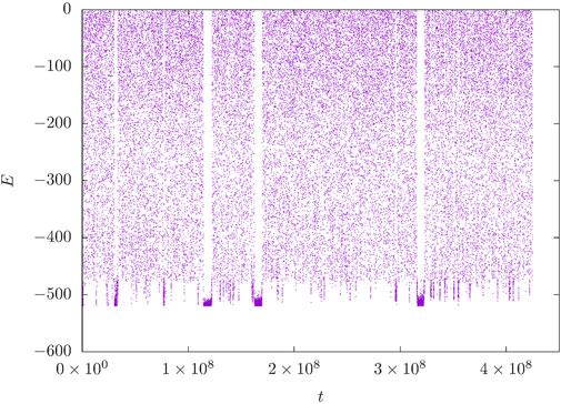
FIGURE 1. Time series of the energy E throughout a simulation of N = 100 Lennard-Jones particles. The energy was restricted to E > − 520.

FIGURE 2

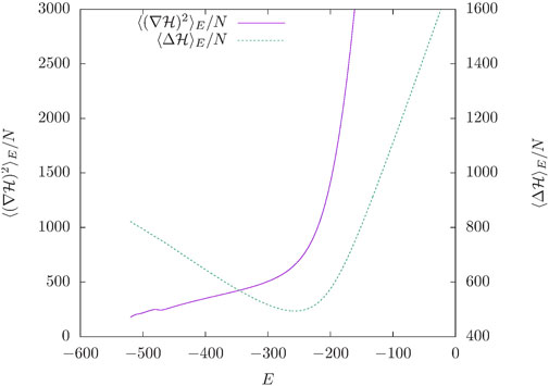
FIGURE 2. The microcanonical averages ${⟨{(\nabla \mathcal{H})}^2⟩}_E/N$ and ${⟨\mathrm{\Delta }\mathcal{H}⟩}_E/N$ from the same simulation as the data in Figure 1.

FIGURE 3

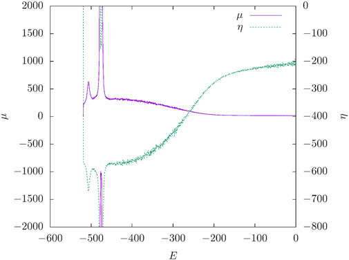
FIGURE 3. The integration parameters μ and η from the same simulation as the data in Figure 1.

5 O(n) spin model

The O(n) spin model is the generalization of the Ising (n = 1), XY (n = 2), and Heisenberg (n = 3) spin models. In this model spins $\mathit{\sigma }\in {\mathbb{R}}^n,|\mathit{\sigma }|=1$ are elements of the n-sphere and are positioned on sites of regular lattices and interact through the Hamiltonian

$\mathcal{H}=-J\sum _{⟨ij⟩}{\mathit{\sigma }}_i{\mathit{\sigma }}_j,(39)$

where the sum runs over all lattice bonds and J is the spin-spin interaction strength. To evaluate $\nabla \mathcal{H}$ and $\mathrm{\Delta }\mathcal{H}$ we first consider the contribution to the total energy by an individual spin σ_k:

$e_k=-{\mathit{\sigma }}_k{\mathbf{h}}_k/|{\mathit{\sigma }}_k|,(40)$

where h_k is the local field

${\mathbf{h}}_k=J\sum _{j\in nb\left(k\right)}{\mathit{\sigma }}_j(41)$

and nb(k) the set of neighbors of spin σ_k. In the following, we set J = 1 and refrain from displaying it in the formulae. This is equivalent to assuming that e_k, h_k, and E are measured in units of J. It is convenient to divide by |σ_k| in Eq. 40 and for the moment to relax the n-sphere constraint to |σ_k| ≠ 1 since this allows one to use the one-particle gradient ${\nabla }_k={(\frac{\partial }{\partial {\mathit{\sigma }}_{k,1}},\dots ,\frac{\partial }{\partial {\mathit{\sigma }}_{k,n}})}^T$ in Cartesian coordinates with the radial component σ_k(∇_ke_k) ensured to be zero. We find that

${\nabla }_k{e}_k{|}_{|{\mathit{\sigma }}_k|=1}=-({\mathbf{h}}_k-\left({\mathbf{h}}_k{\mathit{\sigma }}_k\right){\mathit{\sigma }}_k),(42)$

and since h_k − (h_kσ_k)σ_k, (h_kσ_k)σ_k, and h_k form a right-angled triangle it follows ³

${\left({\nabla }_k{e}_k{|}_{|{\mathit{\sigma }}_k|=1}\right)}^2={\mathbf{h}}_k^2-{\left({\mathbf{h}}_k{\mathit{\sigma }}_k\right)}^2,(43)$

$={\mathbf{h}}_k^2-e_k^2.(44)$

If the system is homogeneous, i.e., if all spins are equivalent we can drop the index k, and if the total number of spins is given by N it is

${⟨{\left(\nabla \mathcal{H}\right)}^2⟩}_E=N\left({⟨{\mathbf{h}}^2⟩}_E-{⟨e^2⟩}_E\right).(45)$

Next, we calculate that

${\mathrm{\Delta }}_k{e}_k{|}_{|{\mathit{\sigma }}_k|=1}={\nabla }_k^2{e}_k{|}_{|{\mathit{\sigma }}_k|=1}=-\left(n-1\right)e_k(46)$

and noting that ⟨e⟩_E = 2E/N we find

${\langle \mathrm{\Delta }\mathcal{H}\rangle }_E=-N\left(n-1\right){\langle e\rangle }_E,(47)$

$=-2\left(n-1\right)E.(48)$

Finally, we arrive at the surprisingly simple result

$g\left(E\right)\propto \frac{1}{{\langle {\mathbf{h}}^2\rangle }_E-{\langle e^2\rangle }_E}\exp \left({\int }_{E_0}^E\frac{-2\left(n-1\right)E^{\prime }/N}{{\langle {\mathbf{h}}^2\rangle }_{E^{\prime }}-{\langle e^2\rangle }_{E^{\prime }}}\mathrm{d}{E}^{\prime }\right).(49)$

Unfortunately, this formula does not generalize to the Ising model n = 1 since on the one hand a continuous energy scale is implicitly required and on the other hand for the Ising model ${⟨{\mathbf{h}}^2⟩}_E={⟨e^2⟩}_E$.

We now consider hypercubic lattices in D dimensions with linear extension L, N = L^D spins, and periodic boundary conditions. For these lattices, the number of neighbors of any site (spin), the so-called coordination number, is z = 2D. During the simulation, we use N bins and integrate after every 10³N individual spin updates. The single concern for selecting this value was to choose it large enough to not slow down the simulation by the computational effort of integrating. Proposed values for spins are selected randomly and independently of the current value. They are drawn using the rejection method for n = 2, Marsaglia’s methods [21] for n = 3, 4 and our own technique [22] for n ≥ 5. Time series of the energy per bond 2E/zN for different values of D and n and about N ≈ 10³ spins are shown in Figure 4. For these cases, the simulation is able to cover most of the available energy interval within about 10⁷ sweeps. We point out that for all simulations shown the ratio between the maximum of the DoS and the minimal value reached is between 10⁷⁸⁰ and 10²⁰⁰⁰. Of course, such values can also be achieved with established state-of-the-art flat-histogram methods, but it is satisfying that this is possible with this method as well since it implies that the integration is done with adequate accuracy. The simulations fall a little bit short of the extremal energies E_max = −E_min = ND. We suspect that one reason is the comparatively large bin width which can become problematic if G or its derivative becomes very steep. From the measured densities of states $g(E)\propto \exp [G(E)]/{⟨{(\nabla \mathcal{H})}^2⟩}_E$ shown in Figure 5 it becomes apparent that due to the relatively low number of just 1000 bins, values in adjacent bins can differ by more than 20 orders of magnitude. It is satisfying that thanks to the linear interpolation of G(E) a relatively flat distribution inside the bins can be maintained regardless and transitions between the bins are still occurring. Another cause for decreasing performance at extremal energies will certainly be the small acceptance rate. Close to the minimal and maximal energy values spins are almost parallel to the local field and since we draw new spin values completely randomly the probability that such a proposal is accepted becomes very small. We refrained from optimizing the simulation since this study is mostly intended as a proof-of-concept.

FIGURE 4

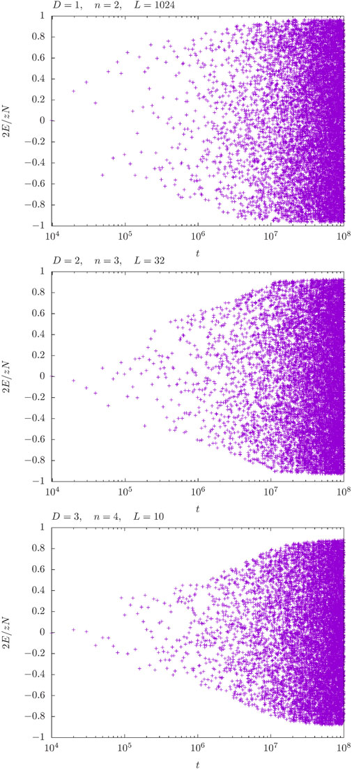
FIGURE 4. Time series of the energy per bond 2E/zN throughout simulations of N ≈ 1000 spins for different values of D and n. The time t is measured in units of N updates.

FIGURE 5

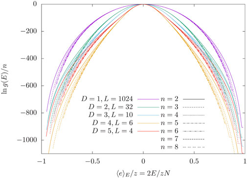
FIGURE 5. Logarithmic density of states divided by n for different sets of values of D, L, and n.

We find that for large enough systems ${⟨h^2⟩}_E$ depends only weakly on the dimension of spin space n. Note that the microcanonical ensemble in the thermodynamic limit directly fixes the correlation between neighboring spins

${⟨{\mathit{\sigma }}_{*}{\mathit{\sigma }}_{|}⟩}_E=-\frac{E}{N}(50)$

and ${⟨h^2⟩}_E$ can be expressed in terms of correlations of next-nearest neighbor spins

${⟨h^2⟩}_E=z+z{⟨{\mathit{\sigma }}_{*}{\mathit{\sigma }}_{\Vert }⟩}_E+z\left(z-2\right){⟨{\mathit{\sigma }}_{*}{\mathit{\sigma }}_{⌞}⟩}_E,(51)$

where from any spin σ_* the spins σ_|, σ_‖, and σ_⌞ are reached by one bond, two parallel bonds and two non-parallel bonds, respectively. This allows one to show that in one dimension ${⟨h^2⟩}_E$ is even independent of n and one obtains

$\underset{N\to \infty }{\lim }{⟨h^2⟩}_E{|}_{D=1}=2+2{\left(E/N\right)}^2(52)$

which is in very good agreement with our data and would be indistinguishable from the graphs for D = 1 in Figure 6. For the other values of D all curves for different n in Figure 6 also are very close to identical. Separate simulations for D = 2, 3 at energies close to the transition revealed that in the thermodynamic limit, the difference in ${⟨h^2⟩}_E$ for different values of n is of the order of 1%. This behavior is reminiscent of another case of unexpectedly small dependence on n: the critical energy density [23].

FIGURE 6

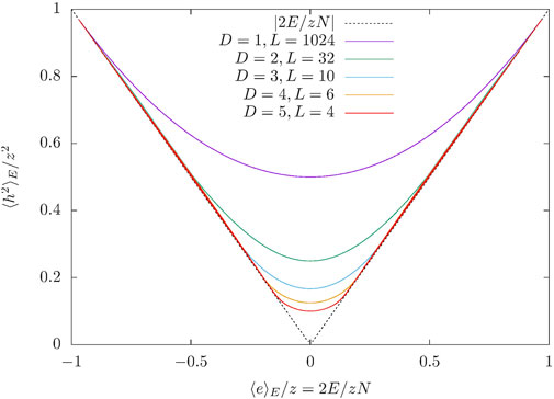
FIGURE 6. Microcanonical average ${⟨h^2⟩}_E$ as function of the energy per bond. For each D curves are shown for n = 2, …, 8 which exhibit hardly any variation.

The situation is different for ${⟨e^2⟩}_E$ which comprises z second moments of nearest-neighbor spin products ${⟨{({\mathit{\sigma }}_k{\mathit{\sigma }}_i)}^2⟩}_E$ as well as z(z − 1) bond-bond correlations ${⟨({\mathit{\sigma }}_k{\mathit{\sigma }}_i)({\mathit{\sigma }}_k{\mathit{\sigma }}_j)⟩}_E$. We are able to calculate the curves for D = 1 and large N analytically, but these do depend on n (see Appendix). The data in Figure 7A suggest that for any D, large n and N an approximation may be given through

${⟨e^2⟩}_E\approx {\left(\frac{2E}{N}\right)}^2+\frac{z{f}_D\left(2E/zN\right)}{n}(53)$

with additional corrections. Here, f_D(x) is a function that can easily be calculated in D = 1 dimension. We find

$f_1\left(x\right)=\frac{{\left(1-x^2\right)}^2}{1+x^2}.(54)$

However, it appears that this function is also valid for D > 1 and we are led to believe by Figure 7B that the next correction is of the order z/n^1/D. This is of course a somewhat speculative heuristic analysis and even though the systems are of medium size N ≈ 10³ the linear extension of the lattices for D > 2 is small.

FIGURE 7

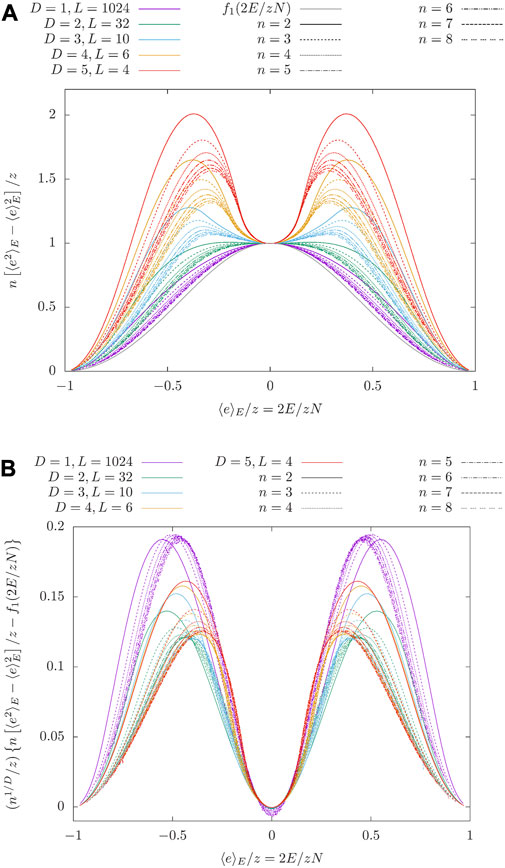
FIGURE 7. (A) The difference of the measured microcanonical average of ${⟨e^2⟩}_E$ and the squared spin energy multiplied by n/z for different sets of values of D, L, n. The gray line represents the theoretical function f₁ for D = 1, n → ∞ and L → ∞ given in Eq. 54. (B) The difference between the data in (A) and f₁ appears to be approximately proportional to z/n^1/D.

Finally we applied the method to the Heisenberg model on a triangular lattice with 1024 spins again with 1000 bins. Now the system experiences frustration at positive energies or negative temperatures which for J = 1 correspond to the antiferromagnet that for this lattice type has a maximal energy 2E_max/zN = 0.5. Again the algorithm is able to explore most of the energy range without getting trapped and the time series (not shown here) looks very similar to the previous cases. In Figure 8 the resulting data for ${⟨h^2⟩}_E$, ${⟨e^2⟩}_E$, and the parameters μ and η are shown.

FIGURE 8

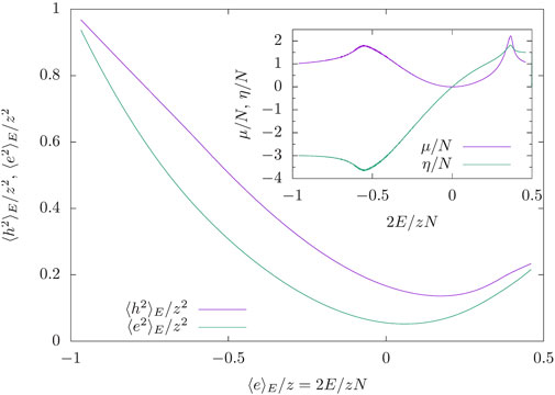
FIGURE 8. Microcanonical averages ${⟨h^2⟩}_E$ and ${⟨e^2⟩}_E$ as a function of the energy per bond for the ferromagnetic (J = 1) Heisenberg model with N = 1024 spins on the triangular lattice (z =6). This system experiences frustration for E > 0. The inset shows the parameters μ and η which as in Figure 3 indicate the positions of phase transitions.

6 Conclusion

In this study, we reviewed how the density of states of a system can be calculated via the inverse microcanonical temperature, i.e., the derivative of the logarithmic density of states, and how the latter can be obtained by means of microcanonical averages. We then introduced an alternative method that avoids mixed derivatives of the Hamiltonian, such that instead of the Hessian only the Laplacian and the gradient are required thus reducing computational demands. Since the ratio of Laplacian and squared gradient needs to be integrated, preferably with high accuracy, we devised a simple method for numerical integration adapted to the mathematical properties of that function.

Once the density of states can be calculated with sufficient accuracy and precision it can be used to verify the results of established histogram-based methods or—as shown in this study—to design a novel flat-distribution Monte Carlo method. This method is similar to the multicanonical method, the Wang-Landau method, or Statistical Temperature MC with the important difference that the information required to bias the ensemble towards a flat distribution is not indirectly obtained through the distribution of energy values but directly measured from the gradient and curvature of the Hamiltonian at the surfaces of constant energy.

The simulations we conducted are intended to be a proof-of-concept and we did not focus on optimizing the algorithm. We deem it likely that improvements can be made in various ways just as there are various histogram-based methods. Even hybrid strategies are conceivable. We observe that the algorithm is able to produce flat histograms on intervals of energy over which the density of states differs by hundreds to thousands of orders of magnitude, which in turn is convincing evidence that our formula for the density of states is correct and that our method for numerical integration works well for this particular type of function.

We applied the method first to a system of one hundred interacting Lennard-Jones particles. In order to ensure a stable simulation and converging microcanonical averages we had to exclude the lowest part of the energy spectrum. Nevertheless, even in the current basic form, the algorithm was able to cover all three phases—gaseous, liquid droplet, and frozen crystal-like—and also managed to map the low-temperature structural transition of the surface atoms. It turned out that the auxiliary data that are produced during the integration can be used to identify the transitions and the energies at which they occur.

Second, we considered the O(n) vector-spin model. After deriving expressions for the Laplacian and gradient of the Hamiltonian it became clear that only the average squared spin energy and the average of the square of a spin’s local field are required to calculate the density of states. Both of these can easily be measured during the simulation. We conducted a number of simulations for various spin and lattice dimensions and system sizes of up to about a thousand spins. In each case, it was easily possible to sample most of the state space. This was even true for the case of a system with frustration: The Heisenberg model on a triangular lattice. We found that the average squared local field depends on D but surprisingly only very little on n. The defining condition of the microcanonical ensemble is of course the system’s fixed total energy which translates to a known value for the nearest-neighbor spin-spin correlation. This in turn is closely related to the quantities needed to calculate the density of states: The squared local field comprises next-nearest-neighbor spin-spin correlations and the squared local energy is the second moment of nearest-neighbor spin products. A more rigorous theoretical analysis of the mutual dependencies of these quantities for the O(n) spin model would be of great interest.

Data availability statement

The raw data supporting the conclusion of this article will be made available by the authors, without undue reservation.

Author contributions

SS developed the method and performed the simulations. WJ and SS reviewed literature compiled and reviewed the manuscript. All authors contributed to the article and approved the submitted version.

Funding

The project was funded by the Deutsche Forschungsgemeinschaft (DFG, German Research Foundation) through the Collaborative Research Centre under Grant No. 189 853 844–SFB/TRR 102 (project B04).

Acknowledgments

SS thanks Franziska Facius for their hospitality.

Conflict of interest

The authors declare that the research was conducted in the absence of any commercial or financial relationships that could be construed as a potential conflict of interest.

Publisher’s note

All claims expressed in this article are solely those of the authors and do not necessarily represent those of their affiliated organizations, or those of the publisher, the editors and the reviewers. Any product that may be evaluated in this article, or claim that may be made by its manufacturer, is not guaranteed or endorsed by the publisher.

Footnotes

¹Here, we assume that the potentials are not uncommonly complicated.

²In each iteration step we perform 1000 N moves, where N is the number of atoms or spins, respectively.

³In the case of the Heisenberg model (n = 3) an alternative expression is ${\mathbf{h}}_k^2-{({\mathbf{h}}_k{\mathit{\sigma }}_k)}^2={({\mathbf{h}}_k\times {\mathit{\sigma }}_k)}^2$ [11].

References

1. Rugh HH. Dynamical approach to temperature. Phys Rev Lett (1997) 78:772–4. doi:10.1103/PhysRevLett.78.772

CrossRef Full Text | Google Scholar

2. Gilat G. Calculation of derivatives of spectral functions in solids. Solid State Commun (1974) 14:263–5. doi:10.1016/0038-1098(74)90849-7

CrossRef Full Text | Google Scholar

3. Butler BD, Ayton G, Jepps OG, Evans DJ. Configurational temperature: Verification of Monte Carlo simulations. J Chem Phys (1998) 109:6519–22. doi:10.1063/1.477301

CrossRef Full Text | Google Scholar

4. Metropolis N, Rosenbluth AW, Rosenbluth MN, Teller AH, Teller E. Equation of state calculations by fast computing machines. J Chem Phys (1953) 21:1087–92. doi:10.1063/1.1699114

CrossRef Full Text | Google Scholar

5. Berg BA, Neuhaus T. Multicanonical algorithms for first order phase transitions. Phys Lett B (1991) 267:249–53. doi:10.1016/0370-2693(91)91256-U

CrossRef Full Text | Google Scholar

6. Wang F, Landau DP. Efficient, multiple-range random walk algorithm to calculate the density of states. Phys Rev Lett (2001) 86:2050–3. doi:10.1103/PhysRevLett.86.2050

PubMed Abstract | CrossRef Full Text | Google Scholar

7. Kim J, Straub JE, Keyes T. Statistical-temperature Monte Carlo and molecular dynamics algorithms. Phys Rev Lett (2006) 97:050601. doi:10.1103/PhysRevLett.97.050601

PubMed Abstract | CrossRef Full Text | Google Scholar

8. Janke W. Histograms and all that. In: B Dünweg, DP Landau, and AI Milchev, editors. Computer simulations of surfaces and interfaces, NATO science series, II. Mathematics, physics and chemistry. Dordrecht: Kluwer (2003). p. 137–57.

CrossRef Full Text | Google Scholar

9. Ferrenberg AM, Swendsen RH. Optimized Monte Carlo data analysis. Phys Rev Lett (1989) 63:1195–8. doi:10.1103/PhysRevLett.63.1195

PubMed Abstract | CrossRef Full Text | Google Scholar

10. Giardina C, Livi R. Ergodic properties of microcanonical observables. J Stat Phys (1998) 91:1027–45. doi:10.1023/A:1023036101468

CrossRef Full Text | Google Scholar

11. Nurdin WB, Schotte K-D. Dynamical temperature for spin systems. Phys Rev E (2000) 61:3579–82. doi:10.1103/PhysRevE.61.3579

PubMed Abstract | CrossRef Full Text | Google Scholar

12. Nurdin WB, Schotte K-D. Dynamical temperature study for classical planar spin systems. Physica A: Stat Mech its Appl (2002) 308:209–26. doi:10.1016/S0378-4371(02)00558-7

CrossRef Full Text | Google Scholar

13. Gutiérrez G, Davis S, Palma G. Configurational temperature in constrained systems: The case of spin dynamics. J Phys A: Math Theor (2018) 51:455003. doi:10.1088/1751-8121/aae163

CrossRef Full Text | Google Scholar

14. Northby JA. Structure and binding of Lennard-Jones clusters: 13 ≤ n ≤ 147. J Chem Phys (1987) 87:6166–77. doi:10.1063/1.453492

CrossRef Full Text | Google Scholar

15. Wales DJ, Doye JPK. Global optimization by basin-hopping and the lowest energy structures of Lennard-Jones clusters containing up to 110 atoms. J Phys Chem A (1997) 101:5111–6. doi:10.1021/jp970984n

CrossRef Full Text | Google Scholar

16. Xiang Y, Jiang H, Cai W, Shao X. An efficient method based on lattice construction and the genetic algorithm for optimization of large Lennard-Jones clusters. J Phys Chem A (2004) 108:3586–92. doi:10.1021/jp037780t

PubMed Abstract | CrossRef Full Text | Google Scholar

17. Mackay AL. A dense non-crystallographic packing of equal spheres. Acta Crystallogr (1962) 15:916–8. doi:10.1107/S0365110X6200239X

CrossRef Full Text | Google Scholar

18. Frantsuzov PA, Mandelshtam VA. Size-temperature phase diagram for small Lennard-Jones clusters. Phys Rev E (2005) 72:037102. doi:10.1103/PhysRevE.72.037102

PubMed Abstract | CrossRef Full Text | Google Scholar

19. Schnabel S, Janke W, Bachmann M. Advanced multicanonical Monte Carlo methods for efficient simulations of nucleation processes of polymers. J Comput Phys (2011) 230:4454–65. doi:10.1016/j.jcp.2011.02.018

CrossRef Full Text | Google Scholar

20. Schnabel S, Seaton DT, Landau DP, Bachmann M. Microcanonical entropy inflection points: Key to systematic understanding of transitions in finite systems. Phys Rev E (2011) 84:011127. doi:10.1103/PhysRevE.84.011127

PubMed Abstract | CrossRef Full Text | Google Scholar

21. Marsaglia G. Choosing a point from the surface of a sphere. Ann Math Stat (1972) 43:645–6. doi:10.1214/aoms/1177692644

CrossRef Full Text | Google Scholar

22. Schnabel S, Janke W. A simple algorithm for uniform sampling on the surface of a hypersphere (2022). arXiv preprint arXiv:2204.14004.

Google Scholar

23. Nerattini R, Trombettoni A, Casetti L. Critical energy density of O(n) models in d = 3. J Stat Mech Theor Exp (2014) 2014:P12001. doi:10.1088/1742-5468/2014/12/P12001

CrossRef Full Text | Google Scholar

Appendix

Calculation of ⟨e²⟩ for D = 1

For D = 1 and large N the spin products σ_k−1σ_k and σ_kσ_k+1 belonging to adjacent bonds are uncorrelated. The average of one product is given by

$Z_n={\int }_{-1}^1{\left(1-s^2\right)}^{\frac{n-3}{2}}{e}^{as}ds,(55)$

To calculate the second moment

$b_2:=⟨{\left({\mathit{\sigma }}_k{\mathit{\sigma }}_{k+1}\right)}^2⟩(56)$

we consider the (reduced) O($n$) partition function

$Z_n={\int }_{-1}^1{\left(1-s^2\right)}^{\frac{n-3}{2}}{e}^{as}ds,(57)$

with s = σ_kσ_k+1 and $a\in (-\infty ,\infty )$. One finds

$Z_2\left(a\right)=\pi I_0\left(a\right),(58)$

$Z_3\left(a\right)=\frac{2\sinh a}{a},(59)$

$Z_4\left(a\right)=\frac{\pi I_1\left(a\right)}{a},(60)$

$Z_5\left(a\right)=4\frac{a\cosh a-\sinh a}{a^3},(61)$

$Z_6\left(a\right)=\frac{3\pi I_2\left(a\right)}{a^2},(62)$

$Z_7\left(a\right)=16\frac{\left(a^2+3\right)\sinh a-3a\cosh a}{a^5},(63)$

$Z_8\left(a\right)=\frac{15\pi I_3\left(a\right)}{a^3},(64)$

$Z_9\left(a\right)=3\frac{32a\left(a^2+15\right)\cosh a-\left(2a^2+5\right)\sinh a}{a^7},(65)$

$Z_{10}\left(a\right)=\frac{105\pi I_4\left(a\right)}{a^4},(66)$

where I_k are modified Bessel functions. It is

$b_1\left(a\right)=\frac{Z_n^{\prime }\left(a\right)}{Z_n\left(a\right)}(67)$

and

$b_2\left(a\right)=\frac{Z_n^{″}\left(a\right)}{Z_n\left(a\right)}(68)$

leading for example with n = 3 to

$b_1\left(a\right)=\frac{\cosh a}{\sinh a}-\frac{1}{a}(69)$

and

$b_2\left(a\right)=1-\frac{2\cosh a}{a\sinh a}+\frac{2}{a^2}=1-2\frac{b_1\left(a\right)}{a}.(70)$

For general n (and D = 1) the second moment of e is given by

$\begin{array}{ll}\hfill {\langle e^2\rangle }_E& =J^2{\langle {\left({\mathit{\sigma }}_{k-1}{\mathit{\sigma }}_k+{\mathit{\sigma }}_k{\mathit{\sigma }}_{k+1}\right)}^2\rangle }_E,\hfill \\ \hfill & =2J^2\left(b_2+b_1^2\right).\hfill \end{array}(71)$

which with Eqs 67, 68 approaches in the limit of large n the closed form expressions Eqs 53, 54 of the main text.