Theoretical study of the interplay of spin density wave and superconductivity in nickel substitution of the strontium–iron–arsenide (SrFe2−xNixAs2) superconductor in a two-band model

1 Introduction

Superconductivity was observed for the first time by a Dutch physicist Heike Kamerlingh Onnes. He found in 1911 that the electrical resistivity of Hg abruptly dropped to zero [1]. After 20 years of his discovery, in 1933, W. Meissner and his student R. Ochsenfeld found that the magnetic field is repelled by superconducting materials, called the Meissner effect [2]. This effect suggests a fundamental property of the superconducting state called perfect diamagnetism. In 1957, L. N. Cooper, J. Bardeen, and J. R. Schrieffer, the three American physicists, developed a quantum theory, called BCS theory, to elucidate the behaviour of superconducting materials at the microscopic level [3]. This theory claims that the formation of quasiparticles termed Cooper pairs by the electrons in a material leads to superconductivity [4]. Cooper pairs are bosons and can aggregate in the same low-energy fundamental state (ground state energy), which is the superconducting state. It bases on a critical assumption that there is an attractive force between electrons. Electrons are fermions and are subject to the Pauli exclusion principle [5].

In the development of condensed matter physics, the discovery of high-transition temperature T_c superconductors marks a turning point. In 1979, the discovery of superconductivity in the heavy-fermion compound, CeCu₂Si₂ [6], came as a surprise because magnetic spin–spin interactions bind the superconducting charge carriers in pair and is highly unlikely by BCS theory [7]. The heavy-fermion system is the first class of unconventional superconductors. K. A. Muller and J. G. Bednorz discovered cuprates, the second class of high-temperature superconductors, in La_2−xBa_xCuO₄ with T_c = 35K [8]. Iron-based superconductors (FebSc), with T_c = 26K in LaOFeAs, are the other family of high-temperature materials. They were identified by Hosono et al., in 2008 [9].

FebScs have various distinct systems that significantly enlarge the class of unconventional superconducting materials. Numerous FebSc systems with various compositions and crystal structure classes are found still now. Different systems are distinguished for convenience by the stoichiometric proportions of the chemical components of their parent molecules [10, 11]. The most common FebSc systems that use this nomenclature are 245, 1144, 42622, 12442, 1111, 111, 11, and 122 (for example, Rb₂Fe₄Se₅, CsEuFe₄As₄, Sr₄V₂O₆Fe₂As₂, RbCa₂Fe₄As₄F₂, SmO_1−xF_xFeAs, NaFeAs, Fe_1+yTe_1−xSe_x, and SrFe_2−xNi_xAs₂) [12–16]. In the 245 FebSc system, Rb₂Fe₄Se₅, there is a unique phase separation phenomenon, unlike most other FebSc systems, and each phase separation has arrived from the competition between magnetic and superconducting ordering in the material [17, 18]. Despite having various structural variations, all FebSc systems have one thing in common: iron-based square-planar sheets [19]. FebSc systems contain iron-based layers, which are essential for their superconductivity, similar to copper oxide-based superconductors, in which oxygen—together with copper—creates the superconductivity layer [20].

According to theories, the parent materials of FebSc are semi-metallic, and the density of state close to Fermi’s surface is primarily supplied by the iron 3d electrons (orbitals) and all five of the 3d orbitals cross Fermi’s surface [21]. Just from the most experimental results and the band structure calculations, the results reveal three iron 3d orbitals (d_xy, d_yz, and d_xz) provide the primary contribution to the density of states near the Fermi level and they ruffle weakly in the z direction [22]. Two electron pockets are situated at the margin of the Brillouin zone (BZ) point, and two hole pockets are distributed evenly throughout the resultant Fermi surface. The weights of the three orbitals, ($d_{x^2-y^2}$, d_yz, and d_xy), are almost equal when doping is near optimum [23]. The two-orbital model and this idea of density of state will be used in this article’s computations.

Within the two-orbital model, the electron Fermi pocket is close to the (π, 0) point and is made up of the orbital d_yz, whereas the hole Fermi pocket around the (0, 0) point is made up of a combination of d_xz and d_yz orbitals. The inter-band spin fluctuation resulting from this nesting is actually the particle hole scattering that occurs between the d_xz and d_yz orbitals since the component of the hole Fermi pocket coupled by the nesting wave vector (π, 0) is primarily of the d_xz orbital characteristic [24]. The amount of doping affects how the electrical band structure is shaped. In electron-doped materials, such as 122 Fe-based superconductor compounds, the Fermi surface has many quasi 2D warped cylinders centred Γ point around (k = 0, 0) and M (k = π, π), as well as a potential quasi 3D pocket close to k_z = π. For electron-doped 122 systems such as SrFe_2−xNi_xAs₂, the electron Fermi pocket expands as the doping level rises, while the hole Fermi pocket contracts until at the strongly doped level, where the hole Fermi pocket eventually disappears. The opposite is true for hole-doped systems [20].

The spin density wave (SDW) state, first proposed by Overhauser in 1962, is where the electronic spin density forms a static wave and makes it a type of anti-ferromagnetic state [25]. It happens in anisotropic low-dimensional compounds at low temperatures. The spin and SDW are coupled. It describes the spin density periodic modulation specified by the Fermi wave number [26]. There is no net magnetization over the entire volume with the density varying perpendicularly as a function of position. When delocalized or itinerant electrons, rather than localized electrons, are responsible for the spatial spin density modulation and the SDW transition takes place. Its origin can be electron–hole pairing or finite wave vector singularities of the magnetic susceptibility [27]. It is Fermi surface nesting that is responsible for SDW stabilization. Nesting of the Fermi surface and SDW are observed in SrFe₂As₂ [28]. Although the SDW transition leads to the establishment of AFM order, which causes the moment of the iron atoms to become still along the longer axis in the orthorhombic phase, and the orthorhombic deformation of the crystal lattice transforms the structure of the crystal from the tetragonal to the orthorhombic phase [29].

The FeAs tetrahedral layers are present in the parent compounds of the 122 iron pnictide superconductors, which also show structural transitions from tetragonal to orthorhombic and from paramagnetic (PM) to anti-ferromagnetic (AFM) structures [30]. It has been demonstrated that the AFM orthorhombic phase is the parent phase of the pnictide superconductor that produces the SDW state, which can be suppressed to produce superconductivity by applying pressure or through chemical doping. It has been demonstrated that the parent pnictide compound structural and magnetic phase transitions are crucial in causing superconductivity [31]. The structural and magnetic transitions in our compound SrFe_2−xNi_xAs₂ occur simultaneously at T_S = T_N ≈ 205K [25, 32, 33]. The transition can be tracked to the concentration x = 0.15, where T_S (T_N) ≈ 40K [34], but T_S (T_N) disappears for x > 0.15 or it is not observed in x = 0.16, which leads to maximum T_c [35]. In the concentration range 0.10 ≤ x ≤ 0.22, superconductivity is observed for SrFe_2−xNi_xAs₂. As the doping level [x in SrFe_2−xNi_xAs₂] increases, the hole Fermi pocket continuously shrinks, whereas the electron pocket becomes larger, and the hole pocket finally vanishes in the heavily doped region, where superconductivity also disappears. Magnetic transition is strongly coupled with the structural distortion. Superconductivity has been demonstrated that the result from the suppression of the AFM state of SrFe₂As₂ by nickel substitution. The suppression of the long-range magnetic ordering and the sudden appearance of the Sc state at the same time are correlated, which suggests that the spin fluctuation of the Fe moments is crucial in creating the superconductive state [36]. The closeness of structural and magnetic transitions suggests that spin and lattice coupling has occurred. Lower symmetry enables the spins to organise and, therefore, reduce magnetic frustrations, which is assumed to be the source of the crystal deformation [37].

FebSc are so interesting because they show the coexistence of superconductivity and magnetism. Therefore, they show a lot of promise for applications. They are desirable for electrical power stations and magnetic applications (Maglev trains) because they have a substantially larger critical magnetic field than cuprates or heavy fermions and high isotropic critical currents. Superconductivity shows potential to have a significant impact on our community and the realisation of a world with minimal carbon emissions [38]. In this article, the researchers study the coexistence of superconductivity and SDW in a two-band model for the iron-based superconductor SrFe_2−xNi_xAs₂ by using Green’s function formalism.

Based on the concepts of electronic structure, this article is investigated theoretically on the coexistence of superconductivity and SDW in nickel substitution of the strontium–iron–arsenide (SrFe_2−xNi_xAs₂) superconductor in a two-band model. By considering a two-band model of Hamiltonian and using the double-time temperature-dependent Green’s function formalism methodology, researchers tried to discover the mathematical statements for the critical temperatures (T_c and T_M) and order parameters (Δ_Sc and M).

2 Mathematical formulation of the problem

We explore a two-band model that encapsulates the fundamental physics of the multi-band unconventional superconducting state and SDW order and has a self-consistent solution in order to investigate the coexistence of superconductivity and SDW. The mean-field model Hamiltonian for the interplay of SDW and superconductivity in our compound in a two-band model (d_yz, say s and d_xz, say d) can be expressed as [39–41]

$\begin{array}{ccc}\hfill \widehat{H}& =\hfill & {\displaystyle \sum _{k,\sigma }}{\epsilon }_s\left(k\right){\widehat{s}}_{k,\sigma }^{†}{\widehat{s}}_{k,\sigma }+{\displaystyle \sum _{k,\sigma }}{\epsilon }_s\left(k\right){\widehat{d}}_{k,\sigma }^{†}{\widehat{d}}_{k,\sigma }-{\mathrm{\Delta }}_{Sc}^s{\displaystyle \sum _k}\left({\widehat{s}}_{k\uparrow }^{†}{\widehat{s}}_{-k\downarrow }^{†}+{\widehat{s}}_{-k\downarrow }{\widehat{s}}_{k\uparrow }\right)\hfill \\ \hfill & \hfill & -{\mathrm{\Delta }}_{Sc}^d{\displaystyle \sum _k}\left({\widehat{d}}_{k\uparrow }^{†}{\widehat{d}}_{-k\downarrow }^{†}+{\widehat{d}}_{-k\downarrow }{\widehat{d}}_{k\uparrow }\right)-{\mathrm{\Delta }}_{Sc}^{sd}{\displaystyle \sum _k}\left({\widehat{s}}_{k\uparrow }^{†}{\widehat{s}}_{-k\downarrow }^{†}+{\widehat{d}}_{-k\downarrow }{\widehat{d}}_{k\uparrow }\right)\hfill \\ \hfill & \hfill & -{\mathrm{\Delta }}_{Sc}^{sd}{\displaystyle \sum _k}\left({\widehat{d}}_{k\uparrow }^{†}{\widehat{d}}_{-k\downarrow }^{†}+{\widehat{s}}_{-k\downarrow }{\widehat{s}}_{k\uparrow }\right)-M{\displaystyle \sum _k}\left({\widehat{s}}_{\left(k+p\right)\uparrow }^{†},{\widehat{d}}_{k\uparrow }+{\widehat{d}}_{\left(k+p\right)\uparrow }^{†},{\widehat{s}}_{k\uparrow }\right),\hfill \end{array}(1)$

where the first term indicates the energy of conduction electrons in the s-band. The second term indicates the energy of conduction electrons in the d-band. The third and fourth terms are the energies involving superconductivity due to the intra-band interactions at the s- and d-bands, respectively. The fifth and sixth terms are the energies involving superconductivity due to the inter-band interaction between bands s and d. The last term is the mean-field Hamiltonian which describes the magnetic interactions. ɛ_s(k) and ɛ_d(k) are energies of an electron measured with respect to the Fermi energy in s and d bands, respectively. ${\widehat{s}}_{k\uparrow }^{†}({\widehat{s}}_{-k\downarrow }^{†})$ are the creation (annihilation) operators in the s-intra-band interaction having the wave number k (−k) and spin ↑ (↓), respectively. ${\widehat{d}}_{k\uparrow }^{†}({\widehat{d}}_{-k\downarrow }^{†})$are the creation (annihilation) operators in the d-intra-band interaction having the wave number k (−k) and spin ↑ (↓), respectively. ${\widehat{s}}_{(k+p)\uparrow }^{†}({\widehat{d}}_{(k+p)\uparrow }^{†})$ are the operators which create fermions with momentum (k + p) in the s(d) band interaction, respectively.

${\mathrm{\Delta }}_{Sc}^s$ is the superconducting order parameter (mean field) due to the intra-band interactions within the s band and is given by

${\mathrm{\Delta }}_{Sc}^s={\displaystyle \sum _k}{U}_s\ll \left({\widehat{s}}_{k\uparrow }^{†},{\widehat{s}}_{-k\downarrow }^{†}\gg \right.,(2)$

where U_s is the intra-band interaction potential in the s-band.

${\mathrm{\Delta }}_{Sc}^d$ is the superconducting order parameter (mean-field) due to the intra-band interactions within the d-band and is given by

${\mathrm{\Delta }}_{Sc}^d={\displaystyle \sum _k}{U}_d\ll \left({\widehat{d}}_{k\uparrow }^{†},{\widehat{d}}_{-k\downarrow }^{†}\gg \right.,(3)$

where U_d is the intra-band interaction potential in the d-band.

${\mathrm{\Delta }}_{Sc}^{sd}$ is the superconducting order parameter (mean-field) due to inter-band interactions between the s- band and d-bands, which is given by

${\mathrm{\Delta }}_{Sc}^{sd}={\displaystyle \sum _k}\frac{U_{sd}}{2}\left(\ll \left({\widehat{s}}_{k\uparrow }^{†},{\widehat{s}}_{-k\downarrow }^{†}\gg +\ll {\widehat{d}}_{k\uparrow }^{†},{\widehat{d}}_{-k\downarrow }^{†}\gg \right)\right.,(4)$

where U_sd is the inter-band interaction potential between the two bands.

The double-time temperature-dependent Green’s function is used to find the equation of motion. This formalism is defined as

$R_r\left(t-t^{\prime }\right)=\ll \widehat{D}\left(t\right),\widehat{E}\left(t^{\prime }\right)\gg =-i\theta \left(t-t^{\prime }\right)⟨\left[\widehat{D}\left(t\right),\widehat{E}\left(t^{\prime }\right)\right]⟩.(5)$

R_r (t − t′) is boson operators’ retarded response function. $⟨\dots ⟩$ and ≪…≫ denote the thermodynamic average and abbreviated notation for the Green’s function in the system, respectively. $\widehat{D}(t)$ and $\widehat{E}(t^{\prime })$ are the Heisenberg notations of the field operators. They are expressed in terms of particle creation and annihilation operators or the quantized field function product. θ(t − t′) represents the Heaviside step function and defined as θ(t − t′) = 1 if t > t′ and 0 if t < t′. $\widehat{D}(t)$ can be written as $\widehat{D}(t)=e^{i\widehat{H}t}D(o)e^{-i\widehat{H}t}$. $\left[\widehat{D}(t),\widehat{E}(t^{\prime })\right]$ is the commutator or anti-commutator. This is described as $\left[\widehat{D}(t),\widehat{E}(t^{\prime })\right]=\widehat{D}(t)\widehat{E}(t^{\prime })-\varsigma \widehat{E}(t^{\prime })\widehat{D}(t)$, where ς = 1 for bosons and ς = −1 for fermions. To obtain the equations of motion, we differentiate Eq. 5 with time (t) as

$\frac{d}{dt}{R}_r(t-t^{\prime })=-\frac{d}{dt}\left(i\theta (t-t^{\prime })⟨\left[\widehat{D}(t),\widehat{E}(t^{\prime })\right]⟩\right)$

$\frac{d}{dt}{R}_r(t-t^{\prime })=-i\frac{d}{dt}\theta (t-t^{\prime })⟨\left[\widehat{D}(t),\widehat{E}(t^{\prime })\right]⟩-i\theta (t-t^{\prime })\frac{d}{dt}⟨\left[\widehat{D}(t),\widehat{E}(t^{\prime })\right]⟩$, and this is simplified to

$i{\dot{R}}_r\left(t-t^{\prime }\right)=\frac{d}{dt}\theta \left(t-t^{\prime }\right)⟨\left[\widehat{D}\left(t\right),\widehat{E}\left(t^{\prime }\right)\right]⟩+\theta \left(t-t^{\prime }\right)\frac{d}{dt}⟨\left[\widehat{D}\left(t\right),\widehat{E}\left(t^{\prime }\right)\right]⟩.(6)$

The Dirac’s delta function δ(t − t′) is related to the Heaviside step function as

$\theta \left(t-t^{\prime }\right)={\int }_{-\infty }^t\delta \left(t-t^{\prime }\right).(7)$

This implies the following:

$\frac{d}{dt}\theta \left(t-t^{\prime }\right)=\delta \left(t-t^{\prime }\right).(8)$

Now let us introduce the Heisenberg equations of motion as

$\frac{d}{dt}\widehat{D}\left(t\right)=\left[\widehat{D}\left(t\right),\widehat{H}\right].(9)$

Substituting Eq. 8 and Eq. 9 into Eq. 6, we have the following:

$i{\dot{R}}_r\left(t-t^{\prime }\right)=\delta \left(t-t^{\prime }\right)⟨\left[\widehat{D}\left(t\right),\widehat{E}\left(t^{\prime }\right)\right]⟩+\ll \left[\widehat{D}\left(t\right),\widehat{H}\right],\widehat{E}\left(t^{\prime }\right)\gg .(10)$

Let R_r(ω) be the Fourier transform of R_r (t − t′), which will be given by

$R_r\left(t-t^{\prime }\right)={\int }_{-\infty }^{\infty }{R}_r\left(\omega \right)e^{-i\omega \left(t-t^{\prime }\right)}d\omega .(11)$

The inverse Fourier transform is

$R_r\left(\omega \right)=\frac{1}{2\pi }{\int }_{-\infty }^{\infty }{R}_r\left(t-t^{\prime }\right)e^{-i\omega \left(t-t^{\prime }\right)}d\left(t-t^{\prime }\right).(12)$

The first-order derivative of Eq. 11 with time will be

$i{\dot{R}}_r\left(t-t^{\prime }\right)=-i\omega {\int }_{-\infty }^{\infty }{R}_r\left(\omega \right)e^{-i\omega \left(t-t^{\prime }\right)}d\omega .(13)$

The Dirac delta function will be defined as

$\delta \left(t-t^{\prime }\right)=\frac{1}{2\pi }{\int }_{-\infty }^{\infty }{e}^{-i\omega \left(t-t^{\prime }\right)}d\omega .(14)$

Substituting Eqs 13, 14 into Eq. 10, we have

$\omega R_r\left(\omega \right)=⟨\left[\widehat{D}\left(t\right),\widehat{E}\left(t^{\prime }\right)\right]⟩+\ll \left[\widehat{D}\left(t\right),\widehat{H}\right],\widehat{E}\left(t^{\prime }\right)\gg .(15)$

Last but not the least, the formalism for the double-time temperature-dependent Green’s function is

$\omega \ll \widehat{D}\left(t\right),\widehat{E}\left(t^{\prime }\right)\gg =⟨\left[\widehat{D}\left(t\right),\widehat{E}\left(t^{\prime }\right)\right]⟩+\ll \left[\widehat{D}\left(t\right),\widehat{H}\right],\widehat{E}\left(t^{\prime }\right)\gg .(16)$

Here, $\ll \widehat{D}(t),\widehat{E}(t^{\prime })\gg$ denotes the Fourier transform of Green’s function involving the operators $\widehat{D}(t)$ and $\widehat{E}(t^{\prime })$. We will apply the anti-commutation relation $\left[{\widehat{s}}_{k\sigma }^{†},{\widehat{s}}_{k{\sigma }^{\prime }}^{†}\right]=\left[{\widehat{s}}_{k\sigma },{\widehat{s}}_{k{\sigma }^{\prime }}\right]=0$ and $\left[{\widehat{s}}_{k\sigma }^{†},{\widehat{s}}_{k{\sigma }^{\prime }}\right]={\delta }_{k{k}^{\prime }}\delta \sigma {\sigma }^{\prime }$ to solve the equation of motion, where ${\delta }_{k{k}^{\prime }}=\left\{\begin{array}{cc}\hfill 1,\hfill & ifk=k^{\prime }\hfill \\ \hfill 0,\hfill & \text{otherwise}\hfill \end{array}\right.$ and $\delta \sigma {\sigma }^{\prime }=\left\{\begin{array}{cc}\hfill 1,\hfill & \sigma ={\sigma }^{\prime }\hfill \\ \hfill 0,\hfill & \text{otherwise}\hfill \end{array}\right.$

For simplification, Eq. 1 can be written as

$\widehat{H}={\widehat{H}}_s+{\widehat{H}}_d+{\widehat{H}}_{sd}+{\widehat{H}}_M,(17)$

where

${\widehat{H}}_s={\displaystyle \sum _{k,\sigma }}{\epsilon }_s\left(k\right){\widehat{s}}_{k,\sigma }^{†}{\widehat{s}}_{k,\sigma }-{\mathrm{\Delta }}_{Sc}^s{\displaystyle \sum _k}\left({\widehat{s}}_{k\uparrow }^{†}{\widehat{s}}_{-k\downarrow }^{†}+{\widehat{s}}_{-k\downarrow }{\widehat{s}}_{k\uparrow }\right).$

This is s intra-band interaction’s mean-field Hamiltonian.

${\widehat{H}}_d={\displaystyle \sum _{k,\sigma }}{\epsilon }_s\left(k\right){\widehat{d}}_{k,\sigma }^{†}{\widehat{d}}_{k,\sigma }-{\mathrm{\Delta }}_{Sc}^d{\displaystyle \sum _k}\left({\widehat{d}}_{k\uparrow }^{†}{\widehat{d}}_{-k\downarrow }^{†}+{\widehat{d}}_{-k\downarrow }{\widehat{d}}_{k\uparrow }\right).$

This is d intra-band interaction’s mean-field Hamiltonian.

${\widehat{H}}_{sd}=-{\mathrm{\Delta }}_{Sc}^{sd}{\displaystyle \sum _k}\left({\widehat{s}}_{k\uparrow }^{†}{\widehat{s}}_{-k\downarrow }^{†}+{\widehat{d}}_{-k\downarrow }{\widehat{d}}_{k\uparrow }\right)-{\mathrm{\Delta }}_{Sc}^{sd}{\displaystyle \sum _k}\left({\widehat{d}}_{k\uparrow }^{†}{\widehat{d}}_{-k\downarrow }^{†}+{\widehat{s}}_{-k\downarrow }{\widehat{s}}_{k\uparrow }\right).$

This is the mean-field Hamiltonian in the inter-band interaction

${\widehat{H}}_M=-M{\displaystyle \sum _k}\left({\widehat{s}}_{\left(k+p\right)\uparrow }^{†},{\widehat{d}}_{k\uparrow }+{\widehat{d}}_{\left(k+p\right)\uparrow }^{†},{\widehat{s}}_{k\uparrow }\right).$

This is the mean-field Hamiltonian due to the magnetic interaction of conduction electrons.

2.1 Superconducting order parameters in the pure superconducting region

2.1.1 ${\mathrm{\Delta }}_{Sc}^s$ due to intra-band interactions within the s-band

To describe the superconducting order parameter due to the intra-band interaction within the s-band in the pure superconducting region, one can use the equation of motion for the correlation $\ll {\widehat{s}}_{k\uparrow }^{†},{\widehat{s}}_{-k\downarrow }^{†}\gg ,$ and the following equation can be written:

$\omega \ll {\widehat{s}}_{k\uparrow }^{†},{\widehat{s}}_{-k\downarrow }^{†}\gg =\left.⟨\left[{\widehat{s}}_{k\uparrow }^{†},{\widehat{s}}_{-k\downarrow }^{†}\right.⟩\right]+\left.\ll {\widehat{s}}_{k\uparrow }^{†},\widehat{H}\right],{\widehat{s}}_{-k\downarrow }^{†}\gg ,(18)$

$\omega \ll {\widehat{s}}_{k\uparrow }^{†},{\widehat{s}}_{-k\downarrow }^{†}\gg =0+\ll \left[{\widehat{s}}_{k\uparrow }^{†},{\widehat{H}}_s+{\widehat{H}}_d+{\widehat{H}}_{sd}+{\widehat{H}}_M\right],{\widehat{s}}_{-k\downarrow }^{†}\gg .(19)$

The commutation relations in Eq. 19 can be solved as follows:$\left[{\widehat{s}}_{k\uparrow }^{†},{\widehat{H}}_s\right]=\left[{\widehat{s}}_{k\uparrow }^{†},{\sum }_{k,\sigma }{\epsilon }_s(k){\widehat{s}}_{k,\sigma }^{†}{\widehat{s}}_{k,\sigma }-{\mathrm{\Delta }}_{Sc}^s{\sum }_k({\widehat{s}}_{k\uparrow }^{†}{\widehat{s}}_{-k\downarrow }^{†}+{\widehat{s}}_{-k\downarrow }{\widehat{s}}_{k\uparrow })\right]\left[{\widehat{s}}_{k\uparrow }^{†},{\widehat{H}}_s\right]={\sum }_{k,\sigma }{\epsilon }_s(k)\left[{\widehat{s}}_{k\uparrow }^{†},{\widehat{s}}_{k,\sigma }^{†}{\widehat{s}}_{k,\sigma }\right]-{\mathrm{\Delta }}_{Sc}^s{\sum }_k(\left[{\widehat{s}}_{k\uparrow }^{†},{\widehat{s}}_{k\uparrow }^{†}{\widehat{s}}_{-k\downarrow }^{†}\right]+\left[{\widehat{s}}_{k\uparrow }^{†},{\widehat{s}}_{-k\downarrow }{\widehat{s}}_{k\uparrow }\right])\left[{\widehat{s}}_{k\uparrow }^{†},{\widehat{H}}_s\right]={\sum }_{k,\sigma }{\epsilon }_s(k)(\left[{\widehat{s}}_{k\uparrow }^{†},{\widehat{s}}_{k,\sigma }^{†}\right]{\widehat{s}}_{k,\sigma }-{\widehat{s}}_{k,\sigma }^{†}\left[{\widehat{s}}_{k\uparrow }^{†},{\widehat{s}}_{k,\sigma }\right])-{\mathrm{\Delta }}_{Sc}^s{\sum }_k\left(\left[{\widehat{s}}_{k\uparrow }^{†},{\widehat{s}}_{k\uparrow }^{†}\right]\right.{\widehat{s}}_{-k\downarrow }^{†}-{\widehat{s}}_{k\uparrow }^{†}\left[{\widehat{s}}_{k\uparrow }^{†},{\widehat{s}}_{-k\downarrow }^{†}\right]+\left[{\widehat{s}}_{k\uparrow }^{†},{\widehat{s}}_{-k\downarrow }\right]{\widehat{s}}_{k\uparrow }-{\widehat{s}}_{-k\downarrow }\left[{\widehat{s}}_{k\uparrow }^{†},{\widehat{s}}_{k\uparrow }\right]$

$\left[{\widehat{s}}_{k\uparrow }^{†},{\widehat{H}}_s\right]=-{\epsilon }_s\left(k\right){\widehat{s}}_{k\uparrow }^{†}+{\mathrm{\Delta }}_{Sc}^s{\widehat{s}}_{-k\downarrow }.(20)$

$\left[{\widehat{s}}_{k\uparrow }^{†},{\widehat{H}}_d\right]=\left[{\widehat{s}}_{k\uparrow }^{†},{\sum }_{k,\sigma }{\epsilon }_s(k){\widehat{d}}_{k,\sigma }^{†}{\widehat{d}}_{k,\sigma }-{\mathrm{\Delta }}_{Sc}^d{\sum }_k\left({\widehat{d}}_{k\uparrow }^{†}{\widehat{d}}_{-k\downarrow }^{†}+{\widehat{d}}_{-k\downarrow }{\widehat{d}}_{k\uparrow }\right]\right.\left[{\widehat{s}}_{k\uparrow }^{†},{\widehat{H}}_d\right]={\sum }_{k,\sigma }{\epsilon }_s(k)(\left[{\widehat{s}}_{k\uparrow }^{†},{\widehat{d}}_{k,\sigma }^{†}{\widehat{d}}_{k,\sigma }\right])-{\mathrm{\Delta }}_{Sc}^d{\sum }_k(\left[{\widehat{s}}_{k\uparrow }^{†},{\widehat{d}}_{k\uparrow }^{†}{\widehat{d}}_{-k\downarrow }^{†}\right]+\left[{\widehat{s}}_{k\uparrow }^{†},{\widehat{d}}_{-k\downarrow }{\widehat{d}}_{k\uparrow }\right])\left[{\widehat{s}}_{k\uparrow }^{†},{\widehat{H}}_d\right]={\sum }_{k,\sigma }{\epsilon }_s(k)(\left[{\widehat{s}}_{k\uparrow }^{†},{\widehat{d}}_{k,\sigma }^{†}\right]{\widehat{d}}_{k,\sigma }-{\widehat{d}}_{k,\sigma }^{†}\left[{\widehat{s}}_{k\uparrow }^{†},{\widehat{d}}_{k,\sigma }\right])-{\mathrm{\Delta }}_{Sc}^d{\sum }_k(\left[{\widehat{s}}_{k\uparrow }^{†},{\widehat{d}}_{k\uparrow }^{†}\right]{\widehat{d}}_{-k\downarrow }^{†}-{\widehat{d}}_{k\uparrow }^{†}\left[{\widehat{s}}_{k\uparrow }^{†},{\widehat{d}}_{-k\downarrow }^{†}\right]+\left[{\widehat{s}}_{k\uparrow }^{†},{\widehat{d}}_{-k\downarrow }\right]{\widehat{d}}_{k\uparrow }-{\widehat{d}}_{-k\downarrow }\left[{\widehat{s}}_{k\uparrow }^{†},{\widehat{d}}_{k\uparrow }\right])$

$\left[{\widehat{s}}_{k\uparrow }^{†},{\widehat{H}}_d\right]=0.(21)$

$\left[{\widehat{s}}_{k\uparrow }^{†},{\widehat{H}}_{sd}\right]=\left[{\widehat{s}}_{k\uparrow }^{†},-{\mathrm{\Delta }}_{Sc}^{sd}{\sum }_k({\widehat{s}}_{k\uparrow }^{†}{\widehat{s}}_{-k\downarrow }^{†}+{\widehat{d}}_{-k\downarrow }{\widehat{d}}_{k\uparrow })-{\mathrm{\Delta }}_{Sc}^{sd}{\sum }_k({\widehat{d}}_{k\uparrow }^{†}{\widehat{d}}_{-k\downarrow }^{†}+{\widehat{s}}_{-k\downarrow }{\widehat{s}}_{k\uparrow })\right]\left[{\widehat{s}}_{k\uparrow }^{†},{\widehat{H}}_{sd}\right]=-{\mathrm{\Delta }}_{Sc}^{sd}{\sum }_k(\left[{\widehat{s}}_{k\uparrow }^{†},{\widehat{d}}_{k\uparrow }^{†}{\widehat{d}}_{-k\downarrow }^{†}\right]+\left[{\widehat{s}}_{k\uparrow }^{†},{\widehat{d}}_{-k\downarrow }{\widehat{d}}_{k\uparrow }\right])-{\mathrm{\Delta }}_{Sc}^{sd}{\sum }_k(\left[{\widehat{s}}_{k\uparrow }^{†},{\widehat{d}}_{k\uparrow }^{†}{\widehat{d}}_{-k\downarrow }^{†}\right]+\left[{\widehat{s}}_{k\uparrow }^{†},{\widehat{s}}_{-k\downarrow }{\widehat{s}}_{k\uparrow }\right])\left[{\widehat{s}}_{k\uparrow }^{†},{\widehat{H}}_{sd}\right]=-{\mathrm{\Delta }}_{Sc}^{sd}{\sum }_k(\left[{\widehat{s}}_{k\uparrow }^{†},{\widehat{d}}_{k\uparrow }^{†}\right]{\widehat{d}}_{-k\downarrow }^{†}-{\widehat{d}}_{k\uparrow }^{†}\left[{\widehat{s}}_{k\uparrow }^{†},{\widehat{d}}_{-k\downarrow }^{†}\right]+\left[{\widehat{s}}_{k\uparrow }^{†},{\widehat{d}}_{-k\downarrow }\right]{\widehat{d}}_{k\uparrow }-{\widehat{d}}_{-k\downarrow }\left[{\widehat{s}}_{k\uparrow }^{†},{\widehat{d}}_{k\uparrow }\right])-{\mathrm{\Delta }}_{Sc}^{sd}{\sum }_k(\left[{\widehat{s}}_{k\uparrow }^{†},{\widehat{d}}_{k\uparrow }^{†}\right]{\widehat{d}}_{-k\downarrow }^{†}-{\widehat{d}}_{k\uparrow }^{†}\left[{\widehat{s}}_{k\uparrow }^{†},{\widehat{d}}_{-k\downarrow }^{†}\right])+\left[{\widehat{s}}_{k\uparrow }^{†},{\widehat{d}}_{-k\downarrow }\right]{\widehat{d}}_{k\uparrow }-{\widehat{d}}_{-k\downarrow }\left.\left[{\widehat{s}}_{k\uparrow }^{†},{\widehat{d}}_{k\uparrow }\right]\right)$

$\left[{\widehat{s}}_{k\uparrow }^{†},{\widehat{H}}_{sd}\right]={\mathrm{\Delta }}_{Sc}^{sd}{\widehat{s}}_{-k\downarrow }.(22)$

$\left[{\widehat{s}}_{k\uparrow }^{†},{\widehat{H}}_M\right]=\left[{\widehat{s}}_{k\uparrow }^{†},-M{\sum }_k\left({\widehat{s}}_{(k+p)\uparrow }^{†}{\widehat{d}}_{k\uparrow }+{\widehat{d}}_{(k+p)\uparrow }^{†}{\widehat{s}}_{k\uparrow }\right.\right]\left[{\widehat{s}}_{k\uparrow }^{†},{\widehat{H}}_M\right]=M{\sum }_k(\left[{\widehat{s}}_{k\uparrow }^{†},{\widehat{s}}_{(k+p)\uparrow }^{†}{\widehat{d}}_{k\uparrow }\right]+\left[{\widehat{s}}_{k\uparrow }^{†},{\widehat{d}}_{(k+p)\uparrow }^{†}{\widehat{s}}_{k\uparrow }\right])\left[{\widehat{s}}_{k\uparrow }^{†},{\widehat{H}}_M\right]=M{\sum }_k(\left[{\widehat{s}}_{k\uparrow }^{†},{\widehat{s}}_{(k+p)\uparrow }^{†}\right]{\widehat{d}}_{k\uparrow }-{\widehat{s}}_{(k+p)\uparrow }^{†}\left[{\widehat{s}}_{k\uparrow }^{†},{\widehat{d}}_{k\uparrow }\right]+\left[{\widehat{s}}_{k\uparrow }^{†},{\widehat{d}}_{(k+p)\uparrow }^{†}\right]{\widehat{s}}_{k\uparrow }-{\widehat{d}}_{(k+p)\uparrow }^{†}\left[{\widehat{s}}_{k\uparrow }^{†},{\widehat{s}}_{k\uparrow }\right])$

$\left[{\widehat{s}}_{k\uparrow }^{†},{\widehat{H}}_M\right]=M{\widehat{d}}_{\left(k+p\right)\uparrow }^{†}.(23)$

Ignoring Eq. 23 and inserting Eq. 20 to Eq. 22 into Eq. 19, we get

$\omega \ll {\widehat{s}}_{k\uparrow }^{†},{\widehat{s}}_{-k\downarrow }^{†}\gg =\ll -{\epsilon }_s\left(k\right){\widehat{s}}_{k\uparrow }^{†}+{\mathrm{\Delta }}_{Sc}^s{\widehat{s}}_{-k\downarrow }+{\mathrm{\Delta }}_{Sc}^{sd}{\widehat{s}}_{-k\downarrow },{\widehat{s}}_{-k\downarrow }^{†}\gg ,(24)$

$\omega \ll {\widehat{s}}_{k\uparrow }^{†},{\widehat{s}}_{-k\downarrow }^{†}\gg =-{\epsilon }_s\left(k\right)\ll {\widehat{s}}_{k\uparrow }^{†},{\widehat{s}}_{-k\downarrow }^{†}\gg +{\mathrm{\Delta }}_{Sc}^s\ll {\widehat{s}}_{-k\downarrow },{\widehat{s}}_{-k\downarrow }^{†}\gg +{\mathrm{\Delta }}_{Sc}^{sd}\ll {\widehat{s}}_{-k\downarrow },{\widehat{s}}_{-k\downarrow }^{†}\gg ,(25)$

$\left(\omega +{\epsilon }_s\left(k\right)\right)\ll {\widehat{s}}_{k\uparrow }^{†},{\widehat{s}}_{-k\downarrow }^{†}\gg =\left({\mathrm{\Delta }}_{Sc}^s+{\mathrm{\Delta }}_{Sc}^{sd}\right)\ll {\widehat{s}}_{-k\downarrow },{\widehat{s}}_{-k\downarrow }^{†}\gg ,(26)$

$\ll {\widehat{s}}_{k\uparrow }^{†},{\widehat{s}}_{-k\downarrow }^{†}\gg =\frac{{\mathrm{\Delta }}_{Sc}^s+{\mathrm{\Delta }}_{Sc}^{sd}}{\omega +{\epsilon }_s\left(k\right)}\ll {\widehat{s}}_{-k\downarrow },{\widehat{s}}_{-k\downarrow }^{†}\gg .(27)$

The equation of motion for the homologous $\ll {\widehat{s}}_{-k\downarrow },{\widehat{s}}_{-k\downarrow }^{†}\gg$ in Eq. 27 is described as

$\omega \ll {\widehat{s}}_{-k\downarrow },{\widehat{s}}_{-k\downarrow }^{†}\gg =\left.⟨\left[{\widehat{s}}_{-k\downarrow },{\widehat{s}}_{-k\downarrow }^{†}\right.⟩\right]+\ll \left[{\widehat{s}}_{-k\downarrow },\widehat{H}\right],{\widehat{s}}_{-k\downarrow }^{†}\gg ,(28)$

$\omega \ll {\widehat{s}}_{-k\downarrow },{\widehat{s}}_{-k\downarrow }^{†}\gg =1+\ll \left[{\widehat{s}}_{-k\downarrow },{\widehat{H}}_s+{\widehat{H}}_d+{\widehat{H}}_{sd}\right],{\widehat{s}}_{-k\downarrow }^{†}\gg .(29)$

Evaluating the commutation relations in Eq. 29 which yields,$\left[{\widehat{s}}_{-k\downarrow },{\widehat{H}}_s\right]=\left[{\widehat{s}}_{-k\downarrow },{\sum }_{k,\sigma }{\epsilon }_s(k){\widehat{s}}_{k,\sigma }^{†}{\widehat{s}}_{k,\sigma }-{\mathrm{\Delta }}_{Sc}^s{\sum }_k({\widehat{s}}_{k\uparrow }^{†}{\widehat{s}}_{-k\downarrow }^{†}+{\widehat{s}}_{-k\downarrow }{\widehat{s}}_{k\uparrow })\right]\left[{\widehat{s}}_{-k\downarrow },{\widehat{H}}_s\right]={\sum }_{k,\sigma }{\epsilon }_s(k)\left[{\widehat{s}}_{-k\downarrow },{\widehat{s}}_{k,\sigma }^{†}{\widehat{s}}_{k,\sigma }\right]-{\mathrm{\Delta }}_{Sc}^s{\sum }_k(\left[{\widehat{s}}_{-k\downarrow },{\widehat{s}}_{k\uparrow }^{†}{\widehat{s}}_{-k\downarrow }^{†}\right]+\left[{\widehat{s}}_{-k\downarrow },{\widehat{s}}_{-k\downarrow }{\widehat{s}}_{k\uparrow }\right])\left[{\widehat{s}}_{-k\downarrow },{\widehat{H}}_s\right]={\sum }_{k,\sigma }{\epsilon }_s(k)(\left[{\widehat{s}}_{-k\downarrow },{\widehat{s}}_{k,\sigma }^{†}\right]{\widehat{s}}_{k,\sigma }-{\widehat{s}}_{k,\sigma }^{†}\left[{\widehat{s}}_{-k\downarrow },{\widehat{s}}_{k,\sigma }\right])-{\mathrm{\Delta }}_{Sc}^s{\sum }_k(\left[{\widehat{s}}_{-k\downarrow },{\widehat{s}}_{k\uparrow }^{†}\right]{\widehat{s}}_{-k\downarrow }^{†}-{\widehat{s}}_{k\uparrow }^{†}\left[{\widehat{s}}_{-k\downarrow },{\widehat{s}}_{-k\downarrow }^{†}\right]+\left[{\widehat{s}}_{-k\downarrow },{\widehat{s}}_{-k\downarrow }\right]{\widehat{s}}_{k\uparrow }-{\widehat{s}}_{-k\downarrow }\left[{\widehat{s}}_{-k\downarrow },{\widehat{s}}_{k\uparrow }\right])$

$\left[{\widehat{s}}_{-k\downarrow },{\widehat{H}}_s\right]={\epsilon }_s\left(k\right){\widehat{s}}_{-k\downarrow }+{\mathrm{\Delta }}_{Sc}^s{\widehat{s}}_{k\uparrow }^{†}.(30)$

$\left[{\widehat{s}}_{-k\downarrow },{\widehat{H}}_d\right]=\left[{\widehat{s}}_{-k\downarrow },{\sum }_{k,\sigma }{\epsilon }_s(k){\widehat{d}}_{k,\sigma }^{†}{\widehat{d}}_{k,\sigma }-{\mathrm{\Delta }}_{Sc}^d{\sum }_k\left({\widehat{d}}_{k\uparrow }^{†}{\widehat{d}}_{-k\downarrow }^{†}+{\widehat{d}}_{-k\downarrow }{\widehat{d}}_{k\uparrow }\right]\right.\left[{\widehat{s}}_{-k\downarrow },,{\widehat{H}}_d\right]={\sum }_{k,\sigma }{\epsilon }_s(k)(\left[{\widehat{s}}_{-k\downarrow },{\widehat{d}}_{k,\sigma }^{†}{\widehat{d}}_{k,\sigma }\right])-{\mathrm{\Delta }}_{Sc}^d{\sum }_k(\left[{\widehat{s}}_{-k\downarrow },{\widehat{d}}_{k\uparrow }^{†}{\widehat{d}}_{-k\downarrow }^{†}\right]+\left[{\widehat{s}}_{-k\downarrow },{\widehat{d}}_{-k\downarrow }{\widehat{d}}_{k\uparrow }\right])\left[{\widehat{s}}_{-k\downarrow },{\widehat{H}}_d\right]={\sum }_{k,\sigma }{\epsilon }_s(k)(\left[{\widehat{s}}_{-k\downarrow },{\widehat{d}}_{k,\sigma }^{†}\right]{\widehat{d}}_{k,\sigma }-{\widehat{d}}_{k,\sigma }^{†}\left[{\widehat{s}}_{-k\downarrow },{\widehat{d}}_{k,\sigma }\right])-{\mathrm{\Delta }}_{Sc}^d{\sum }_k(\left[{\widehat{s}}_{-k\downarrow },{\widehat{d}}_{k\uparrow }^{†}\right]{\widehat{d}}_{-k\downarrow }^{†}-{\widehat{d}}_{k\uparrow }^{†}\left[{\widehat{s}}_{-k\downarrow },{\widehat{d}}_{-k\downarrow }^{†}\right]+\left[{\widehat{s}}_{-k\downarrow },{\widehat{d}}_{-k\downarrow }\right]{\widehat{d}}_{k\uparrow }-{\widehat{d}}_{-k\downarrow }\left[{\widehat{s}}_{-k\downarrow },{\widehat{d}}_{k\uparrow }\right])$

$\left[{\widehat{s}}_{-k\downarrow },{\widehat{H}}_d\right]=0.(31)$

$\left[{\widehat{s}}_{-k\downarrow },{\widehat{H}}_{sd}\right]=\left[{\widehat{s}}_{-k\downarrow },-{\mathrm{\Delta }}_{Sc}^{sd}{\sum }_k({\widehat{s}}_{k\uparrow }^{†}{\widehat{s}}_{-k\downarrow }^{†}+{\widehat{d}}_{-k\downarrow }{\widehat{d}}_{k\uparrow })-{\mathrm{\Delta }}_{Sc}^{sd}{\sum }_k({\widehat{d}}_{k\uparrow }^{†}{\widehat{d}}_{-k\downarrow }^{†}+{\widehat{s}}_{-k\downarrow }{\widehat{s}}_{k\uparrow })\right]\left[{\widehat{s}}_{-k\downarrow },{\widehat{H}}_{sd}\right]=-{\mathrm{\Delta }}_{Sc}^{sd}{\sum }_k(\left[{\widehat{s}}_{-k\downarrow },{\widehat{d}}_{k\uparrow }^{†}{\widehat{d}}_{-k\downarrow }^{†}\right]+\left[{\widehat{s}}_{-k\downarrow },{\widehat{d}}_{-k\downarrow }{\widehat{d}}_{k\uparrow }\right])-{\mathrm{\Delta }}_{Sc}^{sd}{\sum }_k\left(\left[{\widehat{s}}_{-k\downarrow },{\widehat{d}}_{k\uparrow }^{†}{\widehat{d}}_{-k\downarrow }^{†}\right]\right.+\left[\left.{\widehat{s}}_{-k\downarrow },{\widehat{s}}_{-k\downarrow }{\widehat{s}}_{k\uparrow }\right)\right]\left[{\widehat{s}}_{-k\downarrow },{\widehat{H}}_{sd}\right]=-{\mathrm{\Delta }}_{Sc}^{sd}{\sum }_k(\left[{\widehat{s}}_{-k\downarrow },{\widehat{d}}_{k\uparrow }^{†}\right]{\widehat{d}}_{-k\downarrow }^{†}-{\widehat{d}}_{k\uparrow }^{†}\left[{\widehat{s}}_{-k\downarrow },{\widehat{d}}_{-k\downarrow }^{†}\right]+\left[{\widehat{s}}_{-k\downarrow },{\widehat{d}}_{-k\downarrow }\right]{\widehat{d}}_{k\uparrow }-{\widehat{d}}_{-k\downarrow }\left[{\widehat{s}}_{-k\downarrow },{\widehat{d}}_{k\uparrow }\right])\left.-{\mathrm{\Delta }}_{Sc}^{sd}{\sum }_k(\left[{\widehat{s}}_{-k\downarrow },{\widehat{d}}_{k\uparrow }^{†}\right]{\widehat{d}}_{-k\downarrow }^{†}-{\widehat{d}}_{k\uparrow }^{†}\left[{\widehat{s}}_{-k\downarrow },{\widehat{d}}_{-k\downarrow }^{†}\right])+\left[{\widehat{s}}_{-k\downarrow },{\widehat{d}}_{-k\downarrow }\right]{\widehat{d}}_{k\uparrow }-{\widehat{d}}_{-k\downarrow }\left[{\widehat{s}}_{-k\downarrow },{\widehat{d}}_{k\uparrow }\right]\right)$

$\left[{\widehat{s}}_{-k\downarrow },{\widehat{H}}_{sd}\right]={\mathrm{\Delta }}_{Sc}^{sd}{\widehat{s}}_{k\uparrow }^{†}.(32)$

Inserting Eq. 30 to Eq. 32 in Eq. 29, we get

$\omega \ll {\widehat{s}}_{-k\downarrow },{\widehat{s}}_{-k\downarrow }^{†}\gg =1+\ll {\epsilon }_s\left(k\right){\widehat{s}}_{-k\downarrow }+{\mathrm{\Delta }}_{Sc}^s{\widehat{s}}_{k\uparrow }^{†}+{\mathrm{\Delta }}_{Sc}^{sd}{\widehat{s}}_{k\uparrow }^{†},{\widehat{s}}_{-k\downarrow }^{†}\gg ,(33)$

$\omega \ll {\widehat{s}}_{-k\downarrow },{\widehat{s}}_{-k\downarrow }^{†}\gg =1+{\epsilon }_s\left(k\right)\ll {\widehat{s}}_{-k\downarrow },{\widehat{s}}_{-k\downarrow }^{†}\gg +\left({\mathrm{\Delta }}_{Sc}^s+{\mathrm{\Delta }}_{Sc}^{sd}\right)\ll {\widehat{s}}_{k\uparrow }^{†},{\widehat{s}}_{-k\downarrow }^{†}\gg ,(34)$

$\left(\omega -{\epsilon }_s\left(k\right)\right)\ll {\widehat{s}}_{-k\downarrow },{\widehat{s}}_{-k\downarrow }^{†}\gg =1+\left({\mathrm{\Delta }}_{Sc}^s+{\mathrm{\Delta }}_{Sc}^{sd}\right)\ll {\widehat{s}}_{k\uparrow }^{†},{\widehat{s}}_{-k\downarrow }^{†}\gg ,(35)$

$\ll {\widehat{s}}_{-k\downarrow },{\widehat{s}}_{-k\downarrow }^{†}\gg =\frac{1}{\omega -{\epsilon }_s\left(k\right)}+\frac{{\mathrm{\Delta }}_{Sc}^s+{\mathrm{\Delta }}_{Sc}^{sd}}{\omega -{\epsilon }_s\left(k\right)}\ll {\widehat{s}}_{k\uparrow }^{†},{\widehat{s}}_{-k\downarrow }^{†}\gg .(36)$

Substituting Eq. 36 in Eq. 27, we get

$\ll {\widehat{s}}_{k\uparrow }^{†},{\widehat{s}}_{-k\downarrow }^{†}\gg =\left(\frac{{\mathrm{\Delta }}_{Sc}^s+{\mathrm{\Delta }}_{Sc}^{sd}}{\omega +{\epsilon }_s\left(k\right)}\right)\left(\frac{1}{\omega -{\epsilon }_s\left(k\right)}+\frac{{\mathrm{\Delta }}_{Sc}^s+{\mathrm{\Delta }}_{Sc}^{sd}}{\omega -{\epsilon }_s\left(k\right)}\ll {\widehat{s}}_{k\uparrow }^{†},{\widehat{s}}_{-k\downarrow }^{†}\gg \right),(37)$

$\ll {\widehat{s}}_{k\uparrow }^{†},{\widehat{s}}_{-k\downarrow }^{†}\gg =\frac{{\mathrm{\Delta }}_{Sc}^s+{\mathrm{\Delta }}_{Sc}^{sd}}{\left(\omega +{\epsilon }_s\left(k\right)\right)\left(\omega -{\epsilon }_s\left(k\right)\right)}+\left(\frac{{\mathrm{\Delta }}_{Sc}^s+{\mathrm{\Delta }}_{Sc}^{sd}}{\omega +{\epsilon }_s\left(k\right)}\right)\left(\frac{{\mathrm{\Delta }}_{Sc}^s+{\mathrm{\Delta }}_{Sc}^{sd}}{\omega -{\epsilon }_s\left(k\right)}\ll {\widehat{s}}_{k\uparrow }^{†},{\widehat{s}}_{-k\downarrow }^{†}\gg \right),(38)$

$\ll {\widehat{s}}_{k\uparrow }^{†},{\widehat{s}}_{-k\downarrow }^{†}\gg =\frac{{\mathrm{\Delta }}_{Sc}^s+{\mathrm{\Delta }}_{Sc}^{sd}}{\left(\omega +{\epsilon }_s\left(k\right)\right)\left(\omega -{\epsilon }_s\left(k\right)\right)}+\frac{{\left({\mathrm{\Delta }}_{Sc}^s+{\mathrm{\Delta }}_{Sc}^{sd}\right)}^2}{\left(\omega +{\epsilon }_s\left(k\right)\right)\left(\omega -{\epsilon }_s\left(k\right)\right)}\ll {\widehat{s}}_{k\uparrow }^{†},{\widehat{s}}_{-k\downarrow }^{†}\gg ,(39)$

$\left(1-\frac{{\left({\mathrm{\Delta }}_{Sc}^s+{\mathrm{\Delta }}_{Sc}^{sd}\right)}^2}{\left(\omega +{\epsilon }_s\left(k\right)\right)\left(\omega -{\epsilon }_s\left(k\right)\right)}\right)\ll {\widehat{s}}_{k\uparrow }^{†},{\widehat{s}}_{-k\downarrow }^{†}\gg =\frac{{\mathrm{\Delta }}_{Sc}^s+{\mathrm{\Delta }}_{Sc}^{sd}}{\left(\omega +{\epsilon }_s\left(k\right)\right)\left(\omega -{\epsilon }_s\left(k\right)\right)},(40)$

$\frac{\left(\omega +{\epsilon }_s\left(k\right)\right)\left(\omega -{\epsilon }_s\left(k\right)\right)-{\left({\mathrm{\Delta }}_{Sc}^s+{\mathrm{\Delta }}_{Sc}^{sd}\right)}^2}{\left(\omega +{\epsilon }_s\left(k\right)\right)\left(\omega -{\epsilon }_s\left(k\right)\right)}\ll {\widehat{s}}_{k\uparrow }^{†},{\widehat{s}}_{-k\downarrow }^{†}\gg =\frac{{\mathrm{\Delta }}_{Sc}^s+{\mathrm{\Delta }}_{Sc}^{sd}}{\left(\omega +{\epsilon }_s\left(k\right)\right)\left(\omega -{\epsilon }_s\left(k\right)\right)},(41)$

$\ll {\widehat{s}}_{k\uparrow }^{†},{\widehat{s}}_{-k\downarrow }^{†}\gg =\frac{{\mathrm{\Delta }}_{Sc}^s+{\mathrm{\Delta }}_{Sc}^{sd}}{\left(\omega +{\epsilon }_s\left(k\right)\right)\left(\omega -{\epsilon }_s\left(k\right)\right)-{\left({\mathrm{\Delta }}_{Sc}^s+{\mathrm{\Delta }}_{Sc}^{sd}\right)}^2}.(42)$

By ignoring ${\mathrm{\Delta }}_{Sc}^{sd}$, Eq. 42 reduces to the following.

$\ll {\widehat{s}}_{k\uparrow }^{†},{\widehat{s}}_{-k\downarrow }^{†}\gg =\frac{{\mathrm{\Delta }}_{Sc}^s}{\left(\omega +{\epsilon }_s\left(k\right)\right)\left(\omega -{\epsilon }_s\left(k\right)\right)-{\left({\mathrm{\Delta }}_{Sc}^s\right)}^2}.(43)$

By decoupling Eq. 43 using the partial fraction decomposition method, we have

$\ll {\widehat{s}}_{k\uparrow }^{†},{\widehat{s}}_{-k\downarrow }^{†}\gg =\frac{{\mathrm{\Delta }}_{Sc}^s}{\left(\omega +{\epsilon }_s\left(k\right)\right)\left(\omega -{\epsilon }_s\left(k\right)\right)-{\left({\mathrm{\Delta }}_{Sc}^s\right)}^2},(44)$

$\ll {\widehat{s}}_{k\uparrow }^{†},{\widehat{s}}_{-k\downarrow }^{†}\gg =\frac{{\mathrm{\Delta }}_{Sc}^s}{{\omega }^2-{\epsilon }_s^2\left(k\right)-{\left({\mathrm{\Delta }}_{Sc}^s\right)}^2}.(45)$

Using the expression ω → iω_n, where ω_n is the Matsubara frequency and written as

${\omega }_n=\frac{\left(2n+1\right)\pi }{\beta },(46)$

$\ll {\widehat{s}}_{k\uparrow }^{†},{\widehat{s}}_{-k\downarrow }^{†}\gg =-\frac{{\mathrm{\Delta }}_{Sc}^s}{{\omega }_n^2-{\epsilon }_s^2\left(k\right)-{\left({\mathrm{\Delta }}_{Sc}^s\right)}^2},(47)$

$\ll {\widehat{s}}_{k\uparrow }^{†},{\widehat{s}}_{-k\downarrow }^{†}\gg =\frac{{\mathrm{\Delta }}_{Sc}^s}{{\omega }_n^2+{\epsilon }_s^2\left(k\right)+{\left({\mathrm{\Delta }}_{Sc}^s\right)}^2},(48)$

$\ll {\widehat{s}}_{k\uparrow }^{†},{\widehat{s}}_{-k\downarrow }^{†}\gg =\frac{{\mathrm{\Delta }}_{Sc}^s}{{\left(\frac{\left(2n+1\right)\pi }{\beta }\right)}^2+{\epsilon }_s^2\left(k\right)+{\left({\mathrm{\Delta }}_{Sc}^s\right)}^2},(49)$

$\ll {\widehat{s}}_{k\uparrow }^{†},{\widehat{s}}_{-k\downarrow }^{†}\gg =\frac{{\beta }^2{\mathrm{\Delta }}_{Sc}^s}{{\left(\left(2n+1\right)\pi \right)}^2+{\beta }^2\left({\epsilon }_s^2\left(k\right)+{\left({\mathrm{\Delta }}_{Sc}^s\right)}^2\right)}.(50)$

${\mathrm{\Delta }}_{Sc}^s$ is written as

${\mathrm{\Delta }}_{Sc}^s=\frac{U_s}{\beta }{\displaystyle \sum _{k,n}}\ll {\widehat{s}}_{k\uparrow }^{†},{\widehat{s}}_{-k\downarrow }^{†}\gg .(51)$

Substituting Eq. 50 in Eq. 51, we have

${\mathrm{\Delta }}_{Sc}^s=U_s{\displaystyle \sum _{k,n}}\frac{\beta {\mathrm{\Delta }}_{Sc}^s}{{\left(\left(2n+1\right)\pi \right)}^2+{\beta }^2\left({\epsilon }_s^2\left(k\right)+{\left({\mathrm{\Delta }}_{Sc}^s\right)}^2\right)}.(52)$

Let $\xi =\beta \sqrt{{\epsilon }_s^2(k)+{\left({\mathrm{\Delta }}_{Sc}^s\right)}^2}$ and ${\sum }_{-\infty }^{\infty }\frac{1}{{((2n+1)\pi )}^2+{\xi }^2}=\frac{\tanh (\frac{\xi }{2})}{2\xi }$, then Eq. 52 can be written as

${\mathrm{\Delta }}_{Sc}^s=\frac{U_s}{2}{\displaystyle \sum _{k,n}}{\mathrm{\Delta }}_{Sc}^{s}2\beta \frac{\tanh \frac{\xi }{2}}{\xi }.(53)$

Let us change summation into integration in the region −ℏω_F < ɛ_s(k) < ℏω_F, and at the Fermi level, the density of state, N_s(o), is

${\displaystyle \sum _k}\approx {\int }_{-\hslash {\omega }_F}^{\hslash {\omega }_F}{N}_s\left(o\right)d{\epsilon }_s\left(k\right),(54)$

${\mathrm{\Delta }}_{Sc}^s=\frac{U_s}{2}{\int }_{-\hslash {\omega }_F}^{\hslash {\omega }_F}{N}_s\left(o\right){\mathrm{\Delta }}_{Sc}^{s}2\beta \frac{\tanh \frac{\xi }{2}}{\xi }d{\epsilon }_s\left(k\right),(55)$

$\frac{1}{U_s{N}_s\left(o\right)}={\int }_0^{\hslash {\omega }_F}2\beta \frac{\tanh \frac{\xi }{2}}{\xi }d{\epsilon }_s\left(k\right).(56)$

Let α = U_sN_s(o), which is called the superconducting coupling constant in the s-band intra-band interaction.

$\frac{1}{\alpha }={\int }_0^{\hslash {\omega }_F}\frac{\tanh \left(\frac{\beta }{2}{\left({\epsilon }_s^2\left(k\right)+\left({\mathrm{\Delta }}_{Sc}^s\right)\right)}^{\frac{1}{2}}\right)}{{\left({\epsilon }_s^2\left(k\right)+\left({\mathrm{\Delta }}_{Sc}^s\right)\right)}^{\frac{1}{2}}}d{\epsilon }_s\left(k\right).(57)$

Case I: If T → 0, β → ∞ this implies that $\tanh \left(\frac{\beta }{2}{\left({\epsilon }_s^2(k)+\left({\mathrm{\Delta }}_{Sc}^s\right)\right)}^{\frac{1}{2}}\right)\to 1$

$\frac{1}{\alpha }={\int }_0^{\hslash {\omega }_F}\frac{1}{{\left({\epsilon }_s^2\left(k\right)+\left({\mathrm{\Delta }}_{Sc}^s\right)\right)}^{\frac{1}{2}}}d{\epsilon }_s\left(k\right).(58)$

By applying the integral relation $\int \frac{1}{\sqrt{x^{+}{y}^2}}dx=ln\left(x+\sqrt{x^{+}{y}^2}\right)$, Eq. 58 gives

$\frac{1}{\alpha }=ln\left(\frac{\hslash {\omega }_F}{{\mathrm{\Delta }}_{Sc}^s}+{\left({\left(\frac{\hslash {\omega }_F}{{\mathrm{\Delta }}_{Sc}^s}\right)}^2+1\right)}^{\frac{1}{2}}\right),(59)$

$\frac{1}{\alpha }\approx ln\left(2\frac{\hslash {\omega }_F}{{\mathrm{\Delta }}_{Sc}^s}\right),(60)$

${\mathrm{\Delta }}_{Sc}^s=2\hslash {\omega }_{F}exp\left(-\frac{1}{\alpha }\right).(61)$

From the concept of BCS theory, the superconducting order parameter${\mathrm{\Delta }}_{Sc}^s$ at T = 0 for a given superconductor with critical temperature T_c is written as $2{\mathrm{\Delta }}_{Sc}^s(o)=3.53K_B{T}_c$.

$2{\mathrm{\Delta }}_{Sc}^s\left(o\right)=3.53K_B{T}_c=4\hslash {\omega }_{F}exp\left(-\frac{1}{\alpha }\right),(62)$

This gives

$T_c=1.14\frac{\hslash {\omega }_F}{k_B}exp\left(-\frac{1}{U_s{N}_s\left(o\right)}\right),(63)$

where U_s = 0.323meV, N_s(o) = 1.5 (meV)⁻¹, k_B = 0.086 meV/K and ℏω_F = 6 meV [29]. Substituting these experimental values, we get T_c = 10.09K that agrees with the experiment.

Case 2: If 0 < T < T_c, then Eq. 57 is simplified as follows:

$\frac{1}{\alpha }=2\beta {\int }_0^{\hslash {\omega }_F}{\displaystyle \sum _{-\infty }^{\infty }}\frac{1}{{\left(\left(2n+1\right)\pi \right)}^2+{\gamma }^2}d{\epsilon }_s\left(k\right),(64)$

$\frac{1}{\alpha }=\frac{2}{\beta }{\int }_0^{\hslash {\omega }_F}{\displaystyle \sum _{-\infty }^{\infty }}\frac{1}{{\omega }_n^2+{\epsilon }_s^2\left(k\right)+{\left({\mathrm{\Delta }}_{Sc}^s\right)}^2}d{\epsilon }_s\left(k\right).(65)$

From the Laplacian transform with the Matsubara relation result, we can write Eq. 65 as

$\frac{1}{\alpha }=\frac{2}{\beta }{\int }_0^{\hslash {\omega }_F}{\displaystyle \sum _{-\infty }^{\infty }}\frac{1}{{\omega }_n^2+{\epsilon }_s^2\left(k\right)}d{\epsilon }_s\left(k\right)-{\left({\mathrm{\Delta }}_{Sc}^s\right)}^2\frac{2}{\beta }{\int }_0^{\hslash {\omega }_F}{\displaystyle \sum _{-\infty }^{\infty }}\frac{1}{{\omega }_n^2+{\epsilon }_s^2\left(k\right)}d{\epsilon }_s\left(k\right),(66)$

$\begin{array}{ccc}\hfill \frac{1}{\alpha }& =\hfill & 2\beta {\int }_0^{\hslash {\omega }_F}{\displaystyle \sum _{-\infty }^{\infty }}\frac{1}{{\left(2n+1\right)}^2{\pi }^2+{\left(\beta {\epsilon }_s\left(k\right)\right)}^2}d{\epsilon }_s\left(k\right)\hfill \\ \hfill & \hfill & -{\left({\mathrm{\Delta }}_{Sc}^s\right)}^2\frac{2}{\beta }{\int }_0^{\hslash {\omega }_F}{\displaystyle \sum _{-\infty }^{\infty }}\frac{1}{{\left(2n+1\right)}^2\left(\frac{\pi }{\beta }\right)2+{\epsilon }_s^2\left(k\right)}d{\epsilon }_s\left(k\right),\hfill \end{array}(67)$

$\frac{1}{\alpha }={\int }_0^{\hslash {\omega }_F}\frac{\tanh \left(\frac{\beta }{2}{\epsilon }_s\left(k\right)\right)}{{\epsilon }_s^2\left(k\right)}d{\epsilon }_s\left(k\right)-2{\left({\mathrm{\Delta }}_{Sc}^s\right)}^2\frac{2}{\beta }{\int }_0^{\hslash {\omega }_F}{\displaystyle \sum _0^{\infty }}\frac{1}{{\left(2n+1\right)}^2\left(\frac{\pi }{\beta }\right)2+{\epsilon }_s^2\left(k\right)}d{\epsilon }_s\left(k\right).(68)$

Applying the following equality ${\sum }_0^{\infty }\frac{1}{{(y^2+{\epsilon }_s^2(k))}^2}d{\epsilon }_s(k)=2{\sum }_0^{\infty }\frac{1}{y^4{(1+x^2)}^2}d{\epsilon }_s(k)$where $y^2={(2n+1)}^2{(\frac{\pi }{\beta })}^2$ and $x^2=\frac{{\epsilon }_s^2(k)}{y^2}$.

$\frac{1}{\alpha }={\int }_0^{\hslash {\omega }_F}\frac{\tanh \left(\frac{\beta }{2}{\epsilon }_s\left(k\right)\right)}{{\epsilon }_s^2\left(k\right)}d{\epsilon }_s\left(k\right)-{\left({\mathrm{\Delta }}_{Sc}^s\right)}^2\frac{4}{\beta }{\int }_0^{\hslash {\omega }_F}\sum _0^{\infty }\frac{1}{y^4{\left(1+x^2\right)}^2}d{\epsilon }_s\left(k\right).(69)$

From the above equality relations $x=\beta \frac{{\epsilon }_s(k)}{2}$ and $dx=\beta \frac{d{\epsilon }_s(k)}{2}$.

$\frac{1}{\alpha }={\int }_0^{\frac{\beta \hslash {\omega }_F}{2}}\frac{\tanh x}{x}dx-\frac{4}{\beta }{\int }_0^{\infty }{\displaystyle \sum _0^{\infty }}\frac{{\left({\mathrm{\Delta }}_{Sc}^s\right)}^2}{y^3{\left(1+x^2\right)}^2}dx,(70)$

$=\ln \left(\frac{\beta \hslash {\omega }_F}{2}\right)\tanh \left(\frac{\beta \hslash {\omega }_F}{2}\right)-{\int }_0^{\frac{\beta \hslash {\omega }_F}{2}}\frac{lnx}{cos{h}^{2}x}dx-\frac{4{\left({\mathrm{\Delta }}_{Sc}^s\right)}^2}{\beta y^3}{\displaystyle \sum _0^{\infty }}{\int }_0^{\infty }\frac{1}{{\left(1+x^2\right)}^2}dx,(71)$

$=\ln \left(\frac{\beta \hslash {\omega }_F}{2}\right)\tanh \left(\frac{\beta \hslash {\omega }_F}{2}\right)-ln\left(\frac{\pi }{4\gamma }\right)-\frac{4{\beta }^2{\left({\mathrm{\Delta }}_{Sc}^s\right)}^2}{{\pi }^3}{\displaystyle \sum _0^{\infty }}\frac{1}{{\left(2n+1\right)}^3}{\int }_0^{\infty }\frac{1}{{\left(1+x^2\right)}^2}dx,(72)$

$=\ln \left(\frac{\beta \hslash {\omega }_F}{2}\right)\tanh \left(\frac{\beta \hslash {\omega }_F}{2}\right)-ln\left(\frac{\pi }{4\gamma }\right)-\frac{4{\beta }^2{\left({\mathrm{\Delta }}_{Sc}^s\right)}^2}{{\pi }^3}\frac{7}{8}\xi \left(3\right)\frac{\pi }{4}.(73)$

For low temperature, $\tanh (\frac{\beta \hslash {\omega }_F}{2})\to 1$ and γ denotes the Euler’s constant, and its value is given by γ = 1.78. ${\int }_0^{\infty }\frac{1}{{(1+x^2)}^2}dx=\frac{\pi }{4}$ and ${\sum }_0^{\infty }\frac{1}{{(2n+1)}^p}=(1-2^{-p})\xi (p);$ this means ξ(3) = 1.202. So, after some steps, Eq. 73 can be written as

$\frac{1}{\alpha }=ln\left(1.14\frac{\hslash {\omega }_F}{k_B{T}_c}\right)-1.052{\left(\frac{{\mathrm{\Delta }}_{Sc}^s}{\pi k_B{T}_c}\right)}^2.(74)$

From Eq. 74, we have

$\frac{1}{\alpha }=ln\left(1.14\frac{\hslash {\omega }_F}{k_B{T}_c}\right),(75)$

$ln\left(1.14\frac{\hslash {\omega }_F}{k_B{T}_c}\right)=ln\left(1.14\frac{\hslash {\omega }_F}{k_B{T}_c}\right)-1.052{\left(\frac{{\mathrm{\Delta }}_{Sc}^s}{\pi k_B{T}_c}\right)}^2,(76)$

$ln\left(1.14\frac{\hslash {\omega }_F}{k_B{T}_c}\right)-ln\left(1.14\frac{\hslash {\omega }_F}{k_{B}T}\right)=-1.052{\left(\frac{{\mathrm{\Delta }}_{Sc}^s}{\pi k_B{T}_c}\right)}^2,(77)$

$ln\left(\frac{1.14\frac{\hslash {\omega }_F}{k_B{T}_c}}{\left(1.14\frac{\hslash {\omega }_F}{k_{B}T}\right.}\right)=-1.052{\left(\frac{{\mathrm{\Delta }}_{Sc}^s}{\pi k_B{T}_c}\right)}^2,(78)$

$ln\left(\frac{T}{T_c}\right)=-1.052{\left(\frac{{\mathrm{\Delta }}_{Sc}^s}{\pi k_B{T}_c}\right)}^2.(79)$

Using logarithmic series

$ln(\pm k)=\pm k-\frac{1}{2}{k}^2\pm \frac{1}{3}{k}^3-\cdots$

$ln\left(1-\left(1-\frac{T}{T_c}\right)\right)=-\left(1-\frac{T}{T_c}\right)-\frac{1}{2}\left({\left(1-\frac{T}{T_c}\right)}^2\right.-\frac{1}{3}{\left(1-\frac{T}{T_c}\right)}^3-\cdots .(80)$

Leaving the high-order terms, we get the following.

$ln\left(1-\left(1-\frac{T}{T_c}\right)\right)\approx -\left(1-\frac{T}{T_c}\right),(81)$

$-\left(1-\frac{T}{T_c}\right)=-1.052{\left(\frac{{\mathrm{\Delta }}_{Sc}^s}{\pi k_B{T}_c}\right)}^2,(82)$

$1.052\left(\frac{{\mathrm{\Delta }}_{Sc}^s}{\pi k_B{T}_c}\right)={\left(1-\frac{T}{T_c}\right)}^{\frac{1}{2}},(83)$

${\mathrm{\Delta }}_{Sc}^s=\frac{\pi }{1.025}{k}_B{T}_c{\left(1-\frac{T}{T_c}\right)}^{\frac{1}{2}},(84)$

${\mathrm{\Delta }}_{Sc}^s\left(T\right)=3.063k_B{T}_c{\left(1-\frac{T}{T_c}\right)}^{\frac{1}{2}}.(85)$

This equation tells us the superconducting order parameter ${\mathrm{\Delta }}_{Sc}^s$ as a function of temperature. As temperature increases, the order parameter decrease and vanishes at T_c (10.09K). If T is zero, ${\mathrm{\Delta }}_{Sc}^s=2.658meV$.

2.1.2 ${\mathrm{\Delta }}_{Sc}^d$ due to intra-band interactions within the d-band

${\mathrm{\Delta }}_{Sc}^d$ due to the intra-band interactions within the d band provided by

${\mathrm{\Delta }}_{Sc}^d=\frac{U_s}{\beta }{\displaystyle \sum _{k,n}}\ll {\widehat{d}}_{k\uparrow }^{†},{\widehat{d}}_{-k\downarrow }^{†}\gg .(86)$

By applying the same procedure as above, the superconducting transition temperature T_c due to the intra-band interactions within the d-band is written as

$T_c=1.14\frac{\hslash {\omega }_F}{k_B}exp\left(-\frac{1}{U_d{N}_d\left(o\right)}\right),(87)$

where U_d = 0.267meV, N_d(o) = 1.80 (meV)⁻¹, k_B = 0.086 meV/K and ℏω_F = 6 meV [29]. Substituting these experimental values in this equation, we get T_c = 9.92K that agrees with the experiment. The dependence of the superconducting order parameter ${\mathrm{\Delta }}_{Sc}^d$ on temperature due to the intra-band interactions within the d-band is also given by

${\mathrm{\Delta }}_{Sc}^d\left(T\right)=3.063k_B{T}_c{\left(1-\frac{T}{T_c}\right)}^{\frac{1}{2}}.(88)$

Eq. 88 indicates the dependence of the superconducting order parameter on temperature in the d-band intra-band interaction in the pure superconducting region. The superconducting order parameter decreases as the temperature increases. It vanishes at T_c (9.92K). At T = 0, ${\mathrm{\Delta }}_{Sc}^d=2.163meV$.

2.1.3 ${\mathrm{\Delta }}_{Sc}^{sd}$ due to the inter-band interaction between the s- and d-bands

The inter-band interaction between the s- and d-bands causes the superconducting order parameter, which can be connected to Green’s function as

${\mathrm{\Delta }}_{Sc}^{sd}=\frac{U_{sd}}{2}{\displaystyle \sum _k}\left(\ll \left({\widehat{s}}_{k\uparrow }^{†},{\widehat{s}}_{-k\downarrow }^{†}\gg +\ll {\widehat{d}}_{k\uparrow }^{†},{\widehat{d}}_{-k\downarrow }^{†}\gg \right)\right.(89)$

Applying the same procedure, the equation of motion for the correlations $\ll \left({\widehat{s}}_{k\uparrow }^{†},{\widehat{s}}_{-k\downarrow }^{†}\gg \right.$ and $\ll {\widehat{d}}_{k\uparrow }^{†},{\widehat{d}}_{-k\downarrow }^{†}\gg$ to describe the superconducting order parameter by using Green function formalism similar to the previous procedures due to the inter-band interaction is given by

$\ll \left({\widehat{s}}_{k\uparrow }^{†},{\widehat{s}}_{-k\downarrow }^{†}\gg \right.=\frac{{\mathrm{\Delta }}_{Sc}^s+{\mathrm{\Delta }}_{Sc}^{sd}}{(\omega +{\epsilon }_s(k)-M)(\omega -{\epsilon }_s(k)+M)-{\left({\mathrm{\Delta }}_{Sc}^s+{\mathrm{\Delta }}_{Sc}^{sd}\right)}^2}$ and$\ll \left({\widehat{d}}_{k\uparrow }^{†},{\widehat{d}}_{-k\downarrow }^{†}\gg \right.=\frac{{\mathrm{\Delta }}_{Sc}^d+{\mathrm{\Delta }}_{Sc}^{sd}}{(\omega +{\epsilon }_s(k)-M)(\omega -{\epsilon }_s(k)+M)-{\left({\mathrm{\Delta }}_{Sc}^d+{\mathrm{\Delta }}_{Sc}^{sd}\right)}^2}.$

Ignoring the intra-band superconducting order parameter terms and by decoupling these equations using the partial fraction decomposition method, we will have $\ll \left({\widehat{s}}_{k\uparrow }^{†},{\widehat{s}}_{-k\downarrow }^{†}\gg \right.=\frac{1}{2}{\sum }_{i=1}^2\frac{{\beta }^2{\mathrm{\Delta }}_i(k)}{{((2n+1)\pi )}^2+{\beta }^2({\epsilon }_s^2(k)+{\mathrm{\Delta }}_i^2(k))}$ and$\ll \left({\widehat{d}}_{k\uparrow }^{†},{\widehat{d}}_{-k\downarrow }^{†}\gg =\frac{1}{2}{\sum }_{i=1}^2\frac{{\beta }^2{\mathrm{\Delta }}_i(k)}{{((2n+1)\pi )}^2+{\beta }^2({\epsilon }_d^2(k)+{\mathrm{\Delta }}_i^2(k))}\right.$

where ${\mathrm{\Delta }}_i(k)={\mathrm{\Delta }}_{Sc}^{sd}-1{(-1)}^{i}M,$ which is called the effective order parameter. Substituting these equations into Eq. 89, we get

$\begin{array}{ccc}\hfill {\mathrm{\Delta }}_{Sc}^{sd}& =\hfill & \frac{U_{sd}}{2}{\displaystyle \sum _k}\left(\frac{1}{2}{\displaystyle \sum _{i=1}^2}\frac{{\beta }^2{\mathrm{\Delta }}_i\left(k\right)}{{\left(\left(2n+1\right)\pi \right)}^2+{\beta }^2\left({\epsilon }_s^2\left(k\right)+{\mathrm{\Delta }}_i^2\left(k\right)\right)}\right)\hfill \\ \hfill & \hfill & +\frac{U_{sd}}{2}{\displaystyle \sum _k}\left(\frac{1}{2}{\displaystyle \sum _{i=1}^2}\frac{{\beta }^2{\mathrm{\Delta }}_i\left(k\right)}{{\left(\left(2n+1\right)\pi \right)}^2+{\beta }^2\left({\epsilon }_d^2\left(k\right)+{\mathrm{\Delta }}_i^2\left(k\right)\right)}\right).\hfill \end{array}(90)$

Let ɛ_s(k) = ɛ_d(k) in the inter-band interaction between the two bands, and Eq. 90 becomes

${\mathrm{\Delta }}_{Sc}^{sd}=\frac{U_{sd}}{2}{\displaystyle \sum _k}\left(\frac{1}{2}{\displaystyle \sum _{i=\mathrm{1,2}}^2}\frac{{\beta }^2{\mathrm{\Delta }}_i\left(k\right)}{{\left(\left(2n+1\right)\pi \right)}^2+{\beta }^2\left({\epsilon }_s^2\left(k\right)+{\mathrm{\Delta }}_i^2\left(k\right)\right)}\right).(91)$

Let $\mu =\beta \sqrt{{\epsilon }_s^2(k)+{\mathrm{\Delta }}_i^2(k)}$ and ${\sum }_{-\infty }^{\infty }\frac{1}{{((2n+1)\pi )}^2+{\mu }^2}=\frac{\tanh (\frac{\mu }{2})}{2\mu },$ then Eq. 91 is written as

${\mathrm{\Delta }}_{Sc}^{sd}=\frac{U_{sd}}{4}{\displaystyle \sum _{k,i=\mathrm{1,2}}}{\mathrm{\Delta }}_i\left(k\right)\frac{tanh\frac{\beta }{2}\sqrt{\left.{\epsilon }_s^2\left(k\right)+{\mathrm{\Delta }}_i^2\left(k\right)\right)}}{\sqrt{\left.{\epsilon }_s^2\left(k\right)+{\mathrm{\Delta }}_i^2\left(k\right)\right)}}.(92)$

Changing summation into integration in the region −ℏ_F < ɛ_d(k) < ℏω_F, at the Fermi level, the density of state in the inter-band interaction is N_sd(o), that is, ${\sum }_k\approx {\int }_{-\hslash {\omega }_F}^{\hslash {\omega }_F}{N}_{sd}(o)d{\epsilon }_s(k)$ The density of state N_sd(o) is equal to $\sqrt{N_s(o)N_d(o)},$ then Eq. 92 becomes

${\mathrm{\Delta }}_{Sc}^{sd}=\frac{U_{sd}}{4}{\int }_{-\hslash {\omega }_F}^{\hslash {\omega }_F}{N}_{sd}\left(o\right){\mathrm{\Delta }}_i\left(k\right)\frac{tanh\frac{\beta }{2}\sqrt{{\epsilon }_s^2\left(k\right)+{\mathrm{\Delta }}_i^2\left(k\right)}}{\sqrt{{\epsilon }_s^2\left(k\right)+{\mathrm{\Delta }}_i^2\left(k\right)}}d{\epsilon }_s\left(k\right),(93)$

$\frac{2}{U_{sd}\sqrt{N_s{N}_d\left(o\right)}}={\int }_0^{\hslash {\omega }_F}\frac{{\mathrm{\Delta }}_i\left(k\right)}{{\mathrm{\Delta }}_{Sc}^{sd}}\frac{tanh\frac{\beta }{2}\sqrt{{\epsilon }_s^2\left(k\right)+{\mathrm{\Delta }}_i^2\left(k\right)}}{sqrt{\epsilon }_s^2\left(k\right)+{\mathrm{\Delta }}_i^2\left(k\right)}d{\epsilon }_s\left(k\right),(94)$

$\begin{array}{ccc}\hfill \frac{2}{U_{sd}\sqrt{N_s{N}_d\left(o\right)}}={\int }_0^{\hslash {\omega }_F}\left(\frac{{\mathrm{\Delta }}_{Sc}^{sd}-M}{{\mathrm{\Delta }}_{Sc}^{sd}}\right)\frac{tanh\frac{\beta }{2}\sqrt{{\epsilon }_s^2\left(k\right)+{\left({\mathrm{\Delta }}_{Sc}^{sd}-M\right)}^2}}{\sqrt{{\epsilon }_s^2\left(k\right)+{\left({\mathrm{\Delta }}_{Sc}^{sd}-M\right)}^2}}d{\epsilon }_s\left(k\right)& \hfill & \hfill \\ \hfill +{\int }_0^{\hslash {\omega }_F}\left(\frac{{\mathrm{\Delta }}_{Sc}^{sd}-M}{{\mathrm{\Delta }}_{Sc}^{sd}}\right)\frac{tanh\frac{\beta }{2}\sqrt{{\epsilon }_s^2\left(k\right)+{\left({\mathrm{\Delta }}_{Sc}^{sd}-M\right)}^2}}{\sqrt{{\epsilon }_s^2\left(k\right)+{\left({\mathrm{\Delta }}_{Sc}^{sd}-M\right)}^2}}d{\epsilon }_s\left(k\right).& \hfill & \hfill \end{array}(95)$

After a couple of steps, the superconducting transition temperature T_c is given by

$T_c=1.14\frac{\hslash {\omega }_F}{k_B}exp\left(-\frac{1}{U_{sd}\sqrt{N_s{N}_d\left(o\right)}}-\frac{M}{4K_B{T}_c}ln\left(\frac{\hslash {\omega }_F+M}{\hslash {\omega }_F-M}\right)\right),(96)$

where U_sd = 0.297meV, N_d(o) = 1.80 (meV)⁻¹, N_s(o) = 1.5 (meV)⁻¹, k_B = 0.086 meV/K, and ℏω_F = 6 meV [29]. Eq. 96 clearly shows that the superconducting transition temperature depends on the SDW order parameter.

In the pure diamagnetism region M = 0, and Eq. 91 becomes$T_c=1.14\frac{\hslash {\omega }_F}{k_B}exp\left(-\frac{1}{U_{sd}\sqrt{N_s{N}_d(o)}}\right)$ with T_c = 10.20K, which agrees with the experiment.For perfect diamagnetism, M = 0, and after some steps, the superconducting order parameter will be

${\mathrm{\Delta }}_{Sc}^{sd}\left(T\right)=3.063k_B{T}_c{\left(1-\frac{T}{T_c}\right)}^{\frac{1}{2}}.(97)$

This equation shows that the dependence of the superconducting order parameter on the temperature in the inter-band interactions between the s- and d-bands. The superconducting order parameter suppresses as the temperature increases. It vanishes at the superconducting transition temperature (T_c = 10.20K). If $T=0,{\mathrm{\Delta }}_{Sc}^{sd}(0)=2.687meV$.

2.2 SDW order parameter (M)

Using the double-time temperature-dependent Green’s function to the equation of motion for the correlation $\ll {\widehat{s}}_{-(k+p)\uparrow },{\widehat{d}}_{-k\downarrow }^{†}\gg$, we will find the magnetic order parameter. To solve this problem, we start from the equation of motion for the correlation $\ll {\widehat{s}}_{(k+p)\uparrow }^{†},{\widehat{d}}_{-k\downarrow }^{†}\gg ,$ and from double-time temperature-dependent Green’s function, it can be described as

$\omega \ll {\widehat{s}}_{\left(k+p\right)\uparrow }^{†},{\widehat{d}}_{-k\downarrow }^{†}\gg =⟨\left[{\widehat{s}}_{\left(k+p\right)\uparrow }^{†},{\widehat{d}}_{-k\downarrow }^{†}\right]⟩+\ll \left[{\widehat{s}}_{\left(k+p\right)\uparrow }^{†},\widehat{H}\right],{\widehat{d}}_{-k\downarrow }^{†}\gg ,(98)$

$\omega \ll {\widehat{s}}_{\left(k+p\right)\uparrow }^{†},{\widehat{d}}_{-k\downarrow }^{†}\gg =⟨\left[{\widehat{s}}_{\left(k+p\right)\uparrow }^{†},{\widehat{d}}_{-k\downarrow }^{†}\right]⟩+\ll \left[{\widehat{s}}_{\left(k+p\right)\uparrow }^{†},{\widehat{H}}_s+{\widehat{H}}_d+{\widehat{H}}_{sd}+{\widehat{H}}_M\right],{\widehat{d}}_{-k\downarrow }^{†}\gg .(99)$

The commutation relations in Eq. 99 can be solved as follows:

$\left[{\widehat{s}}_{\left(k+p\right)\uparrow }^{†},{\widehat{H}}_s\right]=-{\epsilon }_s\left(k+p\right){\widehat{s}}_{\left(k+p\right)\uparrow }^{†}+{\mathrm{\Delta }}_{Sc}^s{\widehat{s}}_{-\left(k+p\right)\downarrow },(100)$

$\left[{\widehat{s}}_{\left(k+p\right)\uparrow }^{†},{\widehat{H}}_d\right]=0,(101)$

$\left[{\widehat{s}}_{\left(k+p\right)\uparrow }^{†},{\widehat{H}}_{sd}\right]={\mathrm{\Delta }}_{Sc}^{sd}{\widehat{s}}_{-\left(k+p\right)\downarrow },(102)$

$\left[{\widehat{s}}_{\left(k+p\right)\uparrow }^{†},{\widehat{H}}_M\right]=M{\widehat{s}}_{\left(k+p\right)\uparrow }^{†}.(103)$

Substituting Eq. 100 to Eq. 103 in Eq. 99, it gives

$\omega \ll {\widehat{s}}_{\left(k+p\right)\uparrow }^{†},{\widehat{d}}_{-k\downarrow }^{†}\gg =\frac{{\mathrm{\Delta }}_{Sc}^s+{\mathrm{\Delta }}_{Sc}^{sd}}{\omega +{ϵ}_s\left(k+p\right)-M}\ll {\widehat{s}}_{-\left(k+p\right)\downarrow },{\widehat{d}}_{-k\downarrow }^{†}\gg .(104)$

Now, let us find the equation of motion for the correlation $\ll {\widehat{s}}_{-(k+p)\downarrow },{\widehat{d}}_{-k\downarrow }^{†}\gg$ in Eq. 104.

$\omega \ll {\widehat{s}}_{-\left(k+p\right)\downarrow },{\widehat{d}}_{-k\downarrow }^{†}\gg =1+\ll \left[{\widehat{s}}_{-\left(k+p\right)\downarrow },{\widehat{H}}_s+{\widehat{H}}_d+{\widehat{H}}_{sd}+{\widehat{H}}_M\right],{\widehat{d}}_{-k\downarrow }^{†}\gg .(105)$

Solving the commutation relations in Eq. 105, we get

$\left[{\widehat{s}}_{-\left(k+p\right)\downarrow },{\widehat{H}}_s\right]={\epsilon }_s\left(k+p\right){\widehat{s}}_{-\left(k+p\right)\downarrow }+{\mathrm{\Delta }}_{Sc}^s{\widehat{s}}_{\left(k+p\right)\uparrow }^{†},(106)$

$\left[{\widehat{s}}_{-\left(k+p\right)\downarrow },{\widehat{H}}_d\right]=0,(107)$

$\left[{\widehat{s}}_{-\left(k+p\right)\downarrow },{\widehat{H}}_d\right]={\mathrm{\Delta }}_{Sc}^{sd}{\widehat{s}}_{\left(k+p\right)\uparrow }^{†},(108)$

$\left[{\widehat{s}}_{-\left(k+p\right)\downarrow },{\widehat{H}}_d\right]=M{\widehat{s}}_{-\left(k+p\right)\downarrow }.(109)$

Substituting Eq. 106 to Eq. 109 in Eq. 105, we get

$\omega \ll {\widehat{s}}_{-\left(k+p\right)\downarrow },{\widehat{d}}_{-k\downarrow }^{†}\gg =\frac{1}{\omega -\epsilon \left(k+p\right)+M}+\frac{{\mathrm{\Delta }}_{Sc}^s+{\mathrm{\Delta }}_{Sc}^{sd}}{\omega -\epsilon \left(k+p\right)+M}\ll {\widehat{s}}_{\left(k+p\right)\uparrow }^{†},{\widehat{d}}_{-k\downarrow }^{†}\gg .(110)$

Substituting Eq. 110 into Eq. 104 and after some mathematics, we get

$\ll {\widehat{s}}_{-\left(k+p\right)\downarrow },{\widehat{d}}_{-k\downarrow }^{†}\gg =\frac{-\frac{1}{2}\left({\mathrm{\Delta }}_{Sc}^s+M\right)}{-{\omega }^2+{ϵ}_s^2\left(k+p\right)+{\left({\mathrm{\Delta }}_{Sc}^s+M\right)}^2}+\frac{\frac{1}{2}\left({\mathrm{\Delta }}_{Sc}^s-M\right)}{-{\omega }^2+{ϵ}_s^2\left(k+p\right)+{\left({\mathrm{\Delta }}_{Sc}^s-M\right)}^2},(111)$

where ${\mathrm{\Delta }}_j(k)={\mathrm{\Delta }}_{Sc}^{sd}-1{(-1)}^{j}M,$ which is called the effective magnetic order parameter. Using the expression ω → iω_n and applying the nesting condition, ${ϵ}_s^2(k+p)={ϵ}_s^2(k)$. Eq. 111 gives

$\ll {\widehat{s}}_{-\left(k+p\right)\downarrow },{\widehat{d}}_{-k\downarrow }^{†}\gg =\frac{1}{2}{\displaystyle \sum _{j=\mathrm{1,2}}}\frac{{\left(-1\right)}^j{\mathrm{\Delta }}_j\left(k\right)}{{\omega }_n^2+{ϵ}_s^2\left(k\right)+{\mathrm{\Delta }}_j^2\left(k\right)}.(112)$

The magnetic order parameter is given by

$M=\frac{U}{\beta }{\displaystyle \sum _k}\ll {\widehat{s}}_{-\left(k+p\right)\downarrow },{\widehat{d}}_{-k\downarrow }^{†}\gg .(113)$

Substituting Eq. 112 into Eq. 113; transforming summation into integration in the boundary −ℏω_F < ɛ_s(k) < ℏω_F and by presenting the density of state (DOS) at the Fermi level is N(o), that is, ${\sum }_k\approx {\int }_{-\hslash {\omega }_F}^{\hslash {\omega }_F}N(o)d{\epsilon }_s(k),$ and after a couple of steps, we get

$\frac{2}{UN\left(o\right)}=\frac{{\left(-1\right)}^j{\mathrm{\Delta }}_j}{M}{\int }_0^{\hslash {\omega }_F}\frac{tanh\frac{\beta }{2}\sqrt{{\epsilon }_s^2\left(k\right)+{\mathrm{\Delta }}_i^2\left(k\right)}}{\sqrt{{\epsilon }_s^2\left(k\right)+{\mathrm{\Delta }}_i^2\left(k\right)}}d{\epsilon }_s\left(k\right),(114)$

$\begin{array}{ccc}\hfill \frac{2}{UN\left(o\right)}=\frac{-\left({\mathrm{\Delta }}_S^{s}c+M\right)}{M}{\int }_0^{\hslash {\omega }_F}\frac{tanh\frac{\beta }{2}\sqrt{{\epsilon }_s^2\left(k\right)+{\left({\mathrm{\Delta }}_S^{s}c+M\right)}^2}}{\sqrt{{\epsilon }_s^2\left(k\right)+{\left({\mathrm{\Delta }}_S^{s}c+M\right)}^2}}d{\epsilon }_s\left(k\right)& \hfill & \hfill \\ \hfill -\frac{\left({\mathrm{\Delta }}_S^{s}c-M\right)}{M}{\int }_0^{\hslash {\omega }_F}\frac{tanh\frac{\beta }{2}\sqrt{{\epsilon }_s^2\left(k\right)+{\left({\mathrm{\Delta }}_S^{s}c-M\right)}^2}}{\sqrt{{\epsilon }_s^2\left(k\right)+{\left({\mathrm{\Delta }}_S^{s}c-M\right)}^2}}d{\epsilon }_s\left(k\right).& \hfill & \hfill \end{array}(115)$

After some steps, we get

$\frac{1}{UN\left(o\right)}=ln\left(1.14\frac{\hslash {\omega }_F}{k_B{T}_M}\right)-1.052{\left(\frac{M}{\pi k_B{T}_M}\right)}^2+\frac{\beta M}{4}ln\left(\frac{\hslash {\omega }_F+M}{\hslash {\omega }_F-M}\right).(116)$

For small values of M, we ignore the M² term. Thus, Eq. 116 reduces to

$T_M=1.14\frac{\hslash {\omega }_F}{k_B}exp\left(-\frac{1}{UN\left(o\right)}+\frac{\beta M}{4}ln\left(\frac{\hslash {\omega }_F+M}{\hslash {\omega }_F-M}\right)\right),(117)$

where UN(o) = 1.68 [29] and it is the SDW coupling parameter. Eq. 117 shows that the SDW order parameter increases as the SDW transition temperature increases.

For the pure magnetic region ${\mathrm{\Delta }}_{Sc}^s=0$ and Eq. 115 becomes

$\frac{1}{UN\left(o\right)}=-{\int }_0^{\hslash {\omega }_F}\frac{tanh\frac{\beta }{2}\sqrt{{\epsilon }_s^2\left(k\right)+M^2}}{\sqrt{{\epsilon }_s^2\left(k\right)+M^2}}d{\epsilon }_s\left(k\right).(118)$

This is simplified to

$-\frac{1}{UN\left(o\right)}=ln\left(1.14\frac{\hslash {\omega }_F}{k_{B}T}\right)-1.052{\left(\frac{M}{\pi k_{B}T}\right)}^2.(119)$

For a little value of M, M² → 0 and T → T_M. Eq. 119 reduces

$-\frac{1}{UN\left(o\right)}=ln\left(1.14\frac{\hslash {\omega }_F}{k_B{T}_M}\right).(120)$

This implies that

$ln\left(1.14\frac{\hslash {\omega }_F}{k_B{T}_M}\right)=ln\left(1.14\frac{\hslash {\omega }_F}{k_{B}T}\right)-1.052{\left(\frac{M}{\pi k_B{T}_M}\right)}^2.(121)$

Eq. 121 simplifies to

$M=\frac{\pi k_B{T}_M}{1.052}{\left(1-\frac{T}{T_M}\right)}^{\frac{1}{2}},(122)$

$M\left(T\right)=3.063k_B{T}_M{\left(1-\frac{T}{T_M}\right)}^{\frac{1}{2}}.(123)$

Eq. 123 indicates that if temperature rises, the SDW order parameter suppresses.

3 Results and discussion

In this part, we discussed how temperature (T) affects superconducting order parameters (Δ_Sc) and the SDW order parameter (M), and M affects on both the SDW transition temperature (T_M) and superconducting transition temperature (T_c). We expand on the analysis. In a two-band model for SrFe_2−xNi_xAs₂, we created the theoretical examination of the coexistence of superconductivity and SDW. With the aid of a two-band Hamiltonian model and the double-time temperature-dependent Green’s function formal consideration, we were able to derive the mathematical expressions for the superconducting transition temperature (T_c), superconducting order parameters for each intra- and inter-band interactions, SDW order parameter (M), and SDW transition temperature (T_M).

From Eqs 63, 87, 96, we obtain the superconducting transition (critical) temperatures for each intra- and inter-band interactions of SrFe_2−xNi_xAs₂. Using these (T_c) values and Eqs 85, 88, 97, respectively, we plotted the phase diagram of Δ_Sc versus T within each intra-band and inter-band interactions, Figure 1A.

FIGURE 1

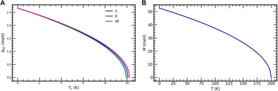
FIGURE 1. Superconducting order parameters vs. temperature for each interactions of the SrFe_2−xNi_xAs₂ superconductor (A) and SDW order parameter (M) vs. temperature in the pure magnetic region of the SrFe_2−xNi_xAs₂ superconductor (B).

As illustrated in Figure 1A, the superconducting order parameter decreases as the temperature increases. It vanishes as the temperature is equal to the critical temperature. For the s intra-band interaction, the maximum value of the superconducting order parameter, $({\mathrm{\Delta }}_{Sc}^s)=2.658meV$, occurs at T = 0, and it vanishes at the superconducting transition temperature T_c = 10.09K. For the d intra-band interaction, the maximum value of the superconducting order parameter,${\mathrm{\Delta }}_{Sc}^d=2.613meV$, occurs at T = 0, and ${\mathrm{\Delta }}_{Sc}^d=0$ at the superconducting transition temperature T_c = 9.92K. Moreover, ${\mathrm{\Delta }}_{Sc}^{sd}=2.687meV$ at T = 0 and ${\mathrm{\Delta }}_{Sc}^{sd}=0$ at the superconducting transition temperature T_c = 10.20K for the inter-band interaction. For each intra-band and inter-band interactions of the SrFe_2−xNi_xAs₂ superconductor, the theoretical values of superconducting transition temperatures agree with the experimental value, which is around T_c = 10K, as discussed in Table 1 [34].

TABLE 1

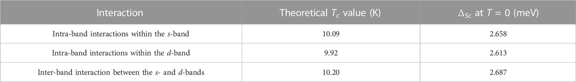
TABLE 1. Superconducting transition temperature T_c values and the superconducting order parameter at T = 0 in different interactions for our compound SrFe_2−xNi_xAs₂. The mean value of T_c is nearly 10K.

Based on Eq. 123, we plotted the phase illustration for the dependence of the magnetic order parameter (M) on temperature in the pure magnetic region illustrated in Figure 1B. As illustrates from this figure, magnetism decreases as the temperature enhances and vanishes at the SDW transition temperature T_M = 205K. The maximum value of the SDW order parameter, M = 54 meV, occurs at T = 0. This finding is also in agreement with experimental observations [34, 37].

Based on Eq. 96, we plotted the phase diagrams of T_c versus M. As illustrated from Figure 2A, when the value of the SDW order parameter enhances, the superconducting transition temperature is suppressed for SrFe_2−xNi_xAs₂. From this figure, one can see the SDW order parameter promotes the magnetic nature and suppresses superconductivity in the system.

FIGURE 2

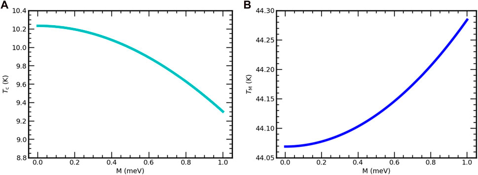
FIGURE 2. Superconducting transition temperature (T_C) versus the SDW order parameter(M) for the inter-band interaction of the SrFe_2−xNi_xAs₂ superconductor (A) and SDW transition temperature (T_M) versus SDW order parameter(M) of SrFe_2−xNi_xAs₂ (B).

Using Eq. 117, we also plotted the phase plotting of the SDW transition temperature (T_M) versus the SDW order parameter (M), as seen in Figure 2B. As demonstrated from this figure, (T_M) progressively gets bigger with the SDW order parameter of the SrFe_2−xNi_xAs₂ superconductor.

Finally, by combining Figures 2A, B, this article depicted a region where both SDW and superconductivity coexist, as shown in Figure 3. Because of their coexistence, the iterating superconducting electrons and spins are thought to have a weak exchange coupling for SrFe_2−xNi_xAs₂. This figure shows that the possible interplay of superconductivity and SDW for SrFe_2−xNi_xAs₂. As indicated in this figure, our finding is in agreement with experimental observations [34, 37]. This figure also depicts there are regions that show the superconducting and anti-ferromagnetic states segregate, which indicates that there are regions where magnetic and superconducting phases are not mixed.

FIGURE 3

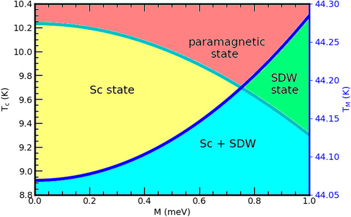
FIGURE 3. Superconducting critical temperature and magnetic transition temperature vs. the SDW order parameter for the SrFe_2−xNi_xAs₂ superconductor.

4 Conclusion

In this work, we have studied the possibility of coexisting superconductivity and magnetism for the iron-based superconductor SrFe_2−xNi_xAs₂. The superconductivity order parameter for FebSc SrFe_2−xNi_xAs₂ is suppressed as the temperature raises and vanishes at the superconducting critical temperature. The magnitude of the SDW order parameter for SrFe_2−xNi_xAs₂ is suppressed as the superconducting critical temperature increases and increases with increasing the SDW transition temperature. We depicted the possibility of coexisting superconductivity and magnetism in the SrFe_2−xNi_xAs₂ superconductor. For the iron-based superconductor SrFe_2−xNi_xAs₂, we further studied the reliance of the SDW order parameter M on temperature in the pure magnetic region. When temperature increases, the SDW order parameter is suppressed and is zero at the SDW transition temperature of the SrFe_2−xNi_xAs₂ superconductor.

Data availability statement

The raw data supporting the conclusion of this article will be made available by the authors, without undue reservation.

Author contributions

All authors listed have made a substantial, direct, and intellectual contribution to the work and approved it for publication.

Conflict of interest

The authors declare that the research was conducted in the absence of any commercial or financial relationships that could be construed as a potential conflict of interest.

Publisher’s note

All claims expressed in this article are solely those of the authors and do not necessarily represent those of their affiliated organizations, or those of the publisher, the editors, and the reviewers. Any product that may be evaluated in this article, or claim that may be made by its manufacturer, is not guaranteed or endorsed by the publisher.

References

1. John R. Solid state physics 1st ed. India: New Delhi McGraw-Hill Education (2014). p. 24. 110016.

Google Scholar

2. Kim CJ, Kim CJ. History of superconductivity Singapore. Superconductor Levitation: Concepts and Experiments (2019). p. 1–11. doi:10.1007/978-981-13-6768-7_1

CrossRef Full Text | Google Scholar

3. Raychaudhuri P, Dutta S. Phase fluctuations in conventional superconductors. J Phys Condensed Matter (2021) 34(8):083001. doi:10.1088/1361-648X/ac360b

CrossRef Full Text | Google Scholar

4. Zhu Z, Papaj M, Nie XA, Xu HK, Gu YS, Yang X, et al. Discovery of segmented Fermi surface induced by Cooper pair momentum. Science (2021) 374(6573):1381–5. doi:10.1126/science.abf1077

PubMed Abstract | CrossRef Full Text | Google Scholar

5. Qiu D, Gong C, Wang S, Zhang M, Yang C, Wang X, et al. Recent advances in 2D superconductors. Adv Mater (2021) 33(18):2006124. doi:10.1002/adma.202006124

CrossRef Full Text | Google Scholar

6. Naqib SH, Islam RS. Possible quantum critical behavior revealed by the critical current density of hole doped high-T c cuprates in comparison to heavy fermion superconductors. Scientific Rep (2019) 9(1):14856. doi:10.1038/s41598-019-51467-4

PubMed Abstract | CrossRef Full Text | Google Scholar

7. Bussmann-Holder A, Keller H. High-temperature superconductors: underlying physics and applications. Z für Naturforschung B (2020) 75(1-2):3–14. doi:10.1515/znb-2019-0103

CrossRef Full Text | Google Scholar

8. Maksimovic N. Advances in nearly-magnetic superconductivity. Berkeley: University of California (2022).

Google Scholar

9. Li H. Spectroscopic–imaging scanning tunneling microscopy studies on cuprates high temperature superconductors. United States: Stony Book Doctoral dissertation, State University of New York at Stony Brook (2021).

Google Scholar

10. Rasaki SA, Thomas T, Yang M. Iron based chalcogenide and pnictide superconductors: from discovery to chemical ways forward. Prog Solid State Chem (2020) 59:100282. doi:10.1016/j.progsolidstchem.2020.100282

CrossRef Full Text | Google Scholar

11. Carretta P, Prando G. Iron-based superconductors: tales from the nuclei. La Rivista Del Nuovo Cimento (2020) 43(1):1–43. doi:10.1007/s40766-019-0001-1

CrossRef Full Text | Google Scholar

12. Fernandes RM, Coldea AI, Ding H, Fisher IR, Hirschfeld PJ, Kotliar G. Iron pnictides and chalcogenides: a new paradigm for superconductivity. Nature (2022) 601(7891):35–44. doi:10.1038/s41586-021-04073-2

PubMed Abstract | CrossRef Full Text | Google Scholar

13. Kreisel A, Hirschfeld PJ, Andersen BM. On the remarkable superconductivity of FeSe and its close cousins. Symmetry (2020) 12(9):1402. doi:10.3390/sym12091402

CrossRef Full Text | Google Scholar

14. Roter B, Ninkovic N, Dordevic SV. Clustering superconductors using unsupervised machine learning. Physica C: Superconductivity its Appl (2022) 598:1354078. doi:10.1016/j.physc.2022.1354078

CrossRef Full Text | Google Scholar

15. Kim TK, Pervakov KS, Evtushinsky DV, Jung SW, Poelchen G, Kummer K, et al. Electronic structure and coexistence of superconductivity with magnetism in RbEuFe₄As₄. Phys Rev B (2021) 103(17):174517. doi:10.1103/PhysRevB.103.174517

CrossRef Full Text | Google Scholar

16. Yu AB, Huang Z, Zhang C, Wu YF, Wang T, Xie T, et al. Superconducting anisotropy and vortex pinning in CaKFe₄As₄ and KCa₂Fe₄As₄F₂. Chin Phys B (2021) 30(2):027401. doi:10.1088/1674-1056/abcf98s

CrossRef Full Text | Google Scholar

17. Park JT, Friemel G, Li Y, Kim JH, Tsurkan V, Deisenhofer J, et al. Magnetic resonant mode in the low energy spin-excitation spectrum of superconducting Rb₂Fe₄Se₅ single crystals. Phys Rev Lett (2011) 107(17):177005. doi:10.1103/physrevlett.107.177005

PubMed Abstract | CrossRef Full Text | Google Scholar

18. Charnukha A, Cvitkovic A, Prokscha T, Propper D, Ocelic N, Suter A, et al. Nanoscale layering of antiferromagnetic and superconducting phases in Rb₂Fe₄Se₅ single crystals. Phys Rev Lett (2012) 109(1):017003. doi:10.1103/PhysRevLett.109.017003

PubMed Abstract | CrossRef Full Text | Google Scholar

19. Gui X, Lv B, Xie W. Chemistry in superconductors. Chem Rev (2021) 121(5):2966–91. doi:10.1021/acs.chemrev.0c00934

PubMed Abstract | CrossRef Full Text | Google Scholar

20. Bogale GM, Shiferaw DA. High entropy materials-microstructures and properties” in iron-based superconductors. Rijeka: Croatia IntechOpen (2022). p. 1–19. doi:10.5772/intechopen.109045

CrossRef Full Text | Google Scholar

21. Ma X, Wang G, Liu R, Yu T, Peng Y, Zheng P, et al. Correlation-corrected band topology and topological surface states in iron-based superconductors. Phys Rev B (2022) 106(11):115114. doi:10.1103/PhysRevB.106.115114

CrossRef Full Text | Google Scholar

22. Tam DW, Berlijn T, Maier TA. Stabilization of s-wave superconductivity through arsenic p-orbital hybridization in electron-doped BaFe 2 as 2. Phys Rev B (2018) 98(2):024507. doi:10.1103/PhysRevB.98.024507

CrossRef Full Text | Google Scholar

23. Zhang R. Neutron scattering studies of the magnetic excitations in 122 family of iron pnictides (doctoral dissertation. Houston: Texas Rice University (2022).

Google Scholar

24. Christensen MH, Kang J, Fernandes RM. Intertwined spin-orbital coupled orders in the iron-based superconductors. Phys Rev B (2019) 100(1):014512. doi:10.1103/PhysRevB.100.014512

CrossRef Full Text | Google Scholar

25. Gruner G. Density waves in solids. Boca Raton: Florida CRC Press (2018). doi:10.1201/9780429501012

CrossRef Full Text | Google Scholar

26. Kokanova SV, Maksimov PA, Rozhkov AV, Sboychakov AO. Competition of spatially inhomogeneous phases in systems with nesting-driven spin-density wave state. Phys Rev B (2021) 104(7):075110. doi:10.1103/PhysRevB.104.075110

CrossRef Full Text | Google Scholar

27. Araujo RDMT, Zarpellon J, Mosca DH. Unveiling ferromagnetism and antiferromagnetism in two dimensions at room temperature. J Phys D: Appl Phys (2022) 55(28):283003. doi:10.1088/1361-6463/ac60cd

CrossRef Full Text | Google Scholar

28. Ali K, Adhikary G, Thakur S, Patil S, Mahatha SK, Thamizhavel A, et al. Hidden phase in parent Fe-pnictide superconductors. Phys Rev B (2018) 97(5):054505. doi:10.1103/PhysRevB.97.054505

CrossRef Full Text | Google Scholar

29. Chen X, Liu N, Guo J, Chen X. Direct response of the spin-density wave transition and superconductivity to anion height in SrFe₂As₂. Phys Rev B (2017) 96(13):134519. doi:10.1103/PhysRevB.96.134519

CrossRef Full Text | Google Scholar

30. Gati E, Xiang L, Bud’ko SL, Canfield PC. Hydrostatic and uniaxial pressure tuning of iron-based superconductors: insights into superconductivity, magnetism, nematicity, and collapsed tetragonal transitions. Annalen der Physik (2020) 532(10):2000248. doi:10.1002/andp.202000248

CrossRef Full Text | Google Scholar

31. Wu JJ, Lin JF, Wang XC, Liu QQ, Zhu JL, Xiao YM, et al. Pressure-decoupled magnetic and structural transitions of the parent compound of iron-based 122 superconductors BaFe₂As₂. Proc Natl Acad Sci (2013) 110(43):17263–6. doi:10.1073/pnas.1310286110

PubMed Abstract | CrossRef Full Text | Google Scholar

32. Chong SV, Tallon JL, Fang F, Kennedy J, Kadowaki K, Williams GVM. Surface superconductivity on SrF e2As2 single crystals induced by ion implantation. EPL (Europhysics Letters) (2011) 94(3):37009. doi:10.1209/0295-5075/94/37009

CrossRef Full Text | Google Scholar

33. Hosono H, Fukuyama H, Akai H. Iron-based superconductors. Handbook Superconductivity: Fundamentals Mater One (2022) 1:293–301. doi:10.1201/9780429179181-30

CrossRef Full Text | Google Scholar

34. Butch NP, Saha SR, Zhang XH, Kirshenbaum K, Greene RL, Paglione J. Effective carrier type and field dependence of the reduced-T c superconducting state in SrFe_2−xNi_xAs₂. Phys Rev B (2010) 81(2):024518. doi:10.1103/PhysRevB.81.024518

CrossRef Full Text | Google Scholar

35. Saha SR, Butch NP, Kirshenbaum K, Paglione J. Annealing effects on superconductivity in SrFe_2−xNi_xAs₂. Physica C, Superconductivity (2010) 470:S379–81. doi:10.1016/j.physc.2009.11.079

CrossRef Full Text | Google Scholar

36. Xie T, Gong D, Ghosh H, Ghosh A, Soda M, Masuda T, et al. Neutron spin resonance in the 112-type iron-based superconductor. Phys Rev Lett (2018) 120(13):137001. doi:10.1103/PhysRevLett.120.137001

PubMed Abstract | CrossRef Full Text | Google Scholar

37. Saha SR, Butch NP, Kirshenbaum K, Paglione J. Evolution of bulk superconductivity in SrFe₂As₂ with Ni substitution. Phys Rev B (2009) 79(22):224519. doi:10.1103/PhysRevB.79.224519

CrossRef Full Text | Google Scholar

38. Yao C, Ma Y. Superconducting materials: challenges and opportunities for large-scale applications. Iscience (2021) 24(6):102541. doi:10.1016/j.isci.2021.102541

PubMed Abstract | CrossRef Full Text | Google Scholar

39. Kidanemariam T, Kahsay G, Mebrahtu A. Theoretical investigation of the coexistence of superconductivity and spin density wave (SDW) in two-band model for the iron-based superconductor BaFe₂(As_1−xP_x)₂. The Eur Phys J B (2019) 92(2):39–12. doi:10.1140/epjb/e2019-80638-9

CrossRef Full Text | Google Scholar

40. Han Q, Chen Y, Wang ZD. A generic two-band model for unconventional superconductivity and spin-density-wave order in electron-and hole-doped iron-based superconductors. EPL (Europhysics Letters) (2008) 82(3):37007. doi:10.1209/0295-5075/82/37007

CrossRef Full Text | Google Scholar

41. Mebratie G, Bekele T. Theoretical investigation of the interplay of superconductivity and magnetism in Ba1xKxFe2As2 superconductor in a two-band model by using the bogoliubov transformation formalism. Adv Condensed Matter Phys (2023) 2023:1–14. doi:10.1155/2023/9556764

CrossRef Full Text | Google Scholar