Adding a low frequency limit to fractional wave propagation models

1 Introduction

In many complex elastic media, attenuation of compressional and/or shear waves often follows a power-law. The amplitude as a function of distance, x, for a sinusoidal input of frequency ω, is therefore:

$|u\left(x\right)|\propto {\mathrm{e}}^{-{\alpha }_k\left(\omega \right)x},{\alpha }_k\left(\omega \right)={\alpha }_0{\omega }^{\alpha +1},(1)$

where α_k(ω) is the attenuation, u is particle displacement, and 0 < α ≤ 1. For many complex media, the attenuation increases with a power close to unity, i.e. α is close to zero [1].

In recent years, it has been found that such power-law attenuation can be obtained as the solution of fractional partial differential equations. These fractional wave equations build on medium models where Newtonian viscosity has been substituted with a more general fractional derivative relationship between stress and strain, see, e.g., Mainardi [2] and Holm [3, Chap. 1].

Although these models may not describe the underlying physics of the wave medium interaction, they are very useful for simulation of wave propagation [4]. Fractional models are also parsimonous descriptions of complex media where the underlying physics is too complex to be described, e.g., in shear wave elastography [5]. Fractional models may also shed light on desirable properties of solutions based on criteria such as causality and passivity of the medium [6].

A more physical model is based on multiple relaxation processes. The elastic wave attenuation resulting from a relaxation process is:

${\alpha }_k\left(\omega \right)=\frac{\mathrm{\Omega }}{{\omega }^2+{\mathrm{\Omega }}^2}{\omega }^2,(2)$

where Ω = 1/τ represents a characteristic relaxation frequency and τ is the relaxation time. This expression increases with ω² in the most important frequency region up to the relaxation frequency and levels off asymptotically to a constant value above the relaxation frequency. As an example, attenuation in seawater can be described by a sum of three such relaxation processes, due respectively, to structural relaxation of water molecules, and chemical relaxation of boric acid and magnesium sulfate [7].

For more complex media, such a finite sum is generalized to an integral over the whole frequency domain with a weighting function A(Ω):

${\alpha }_k\left(\omega \right)={\omega }^2{\int }_0^{\infty }\frac{A\left(\mathrm{\Omega }\right)}{{\omega }^2+{\mathrm{\Omega }}^2}\mathrm{d}\mathrm{\Omega }.(3)$

It can be shown that in order to achieve the power-law attenuation of (Eq. 1) the following weighting function is required [8, 9], Holm [3, Chap. 7]:

$A\left(\mathrm{\Omega }\right)={\mathrm{\Omega }}^{\alpha }.(4)$

This may readily be shown by solving (Eq. 3) as in [10] or by using Gradshteyn and Ryzhik [11, integral 3.241.2].

Often in practice, there are limitations on the relaxation processes in a medium. The most important one is a low-frequency limit. Working in the context of seismology, Futterman [12] analyzed attenuation which increases linearly with frequency. This is also called constant-Q attenuation. He found that in order to satisfy the Kramers–Kronig relations dictated by causality, there has to be a low-frequency cutoff below which attenuation increases faster with frequency. For instance in sediment acoustics, the attenuation follows a steeper power law below a few kHz, Williams et al. [13, Figure 6].

A multiple relaxation distribution may easily be limited so that it has no contributions below a certain frequency Ω_L:

${\alpha }_k\left(\omega \right)={\omega }^2{\int }_{{\mathrm{\Omega }}_L}^{\infty }\frac{A\left(\mathrm{\Omega }\right)}{{\omega }^2+{\mathrm{\Omega }}^2}\mathrm{d}\mathrm{\Omega }.(5)$

The effect of this limit is that attenuation follows frequency squared below Ω_L. This low-frequency limit is not present in the standard fractional models, as they will describe power-law attenuation from 0 frequency to infinity.

Realistically, there is a high-frequency limit also, for instance due to the continuum model breaking down as wavelengths approach molecular dimensions making the distribution of mechanisms unpopulated above some upper frequency limit. The relaxation frequency of structural relaxation in water is near such a limit, see [14] and also the discussion of “fast sound” in water in Holm [Section 4.1.3]. Another high-frequency effect has to do with whether the model’s transient response reaches all over the medium instantaneously or not. If it does, the model is weakly causal, if the transient only reaches the medium for t > 0, it is strongly causal Holm [3, Section 4.2]. In this study, we will focus on this causality property and not possible high-frequency limits.

The purpose of this paper is first to give a brief review of present linear viscoleasticity models, both ordinary and in particular fractional ones, focusing on how they behave for low and high frequencies. The topics of weak and strong causality are of importance here. Second, the purpose is to contribute to better modeling of the band-limited response of Eq. 5 for fractional models. A low-frequency limit can be superimposed on the model by introducing tempering of the medium’s relaxation response, and the effect of that is analyzed.

2 Mechanical medium models

2.1 Standard models

The most general standard model in linear viscoelasticity is the Zener model. The relationship between stress, σ(t), and strain, ϵ(t), is Tschoegl [15, Section 3.4], Mainardi [2, Chap. 2]. Here the terminology follows Holm [3, Chap. 3]:

$\sigma \left(t\right)+{\tau }_{\sigma }\frac{\partial \sigma \left(t\right)}{\partial t}=E_e\left[ϵ\left(t\right)+{\tau }_{ϵ}\frac{\partial ϵ\left(t\right)}{\partial t}\right].(6)$

The two time constants given by the parameters of Figure 1C are:

${\tau }_{\sigma }=\frac{\eta }{E_e}\le {\tau }_{ϵ}=\frac{E+E_e}{E_e}{\tau }_{\sigma },(7)$

where E_e is the equilibrium value for the relaxation modulus, τ_σ is the relaxation time constant, and τ_ϵ is the retardation time constant. The Zener model’s stress response to a unit-step excitation in strain, the relaxation modulus, G(t), is given in Table 1.

FIGURE 1

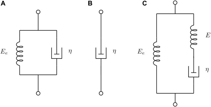
FIGURE 1. Spring-damper representations of constitutive models for viscoelastic media: (A) Kelvin-Voigt, (B) diffusion, and (C) the Zener model.

TABLE 1

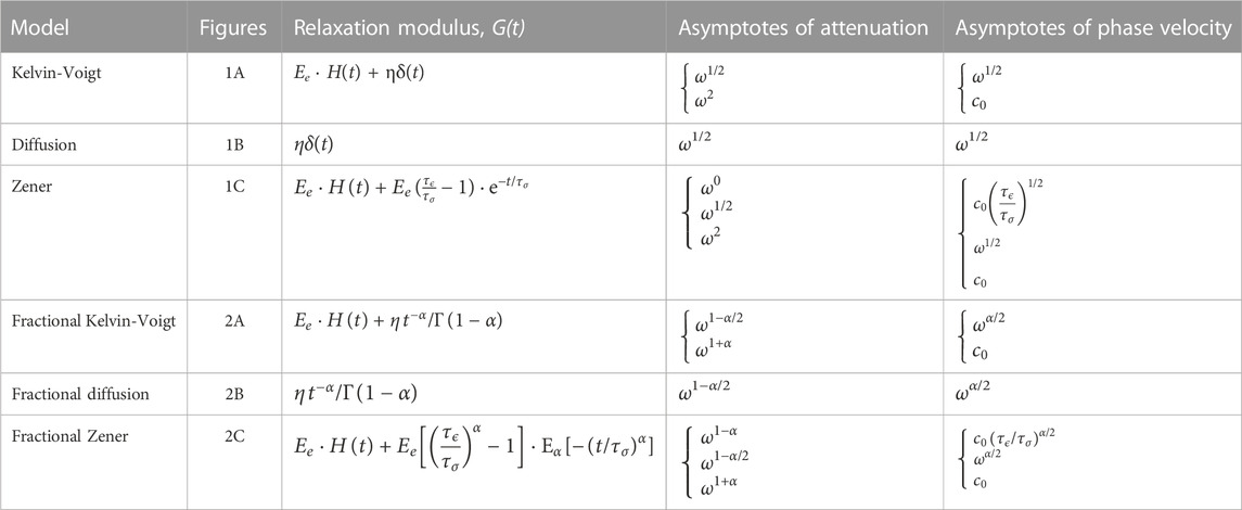
TABLE 1. Relaxation responses for t ≥ 0 with H(t) the Heaviside step function, asymptotes of attenuation and of phase velocity of standard and fractional linear viscoelasticity models. Attenuation and phase velocity asymptotes are shown with the low-frequency asymptote at the bottom and the high-frequency asymptote at the top. Results from Holm [3, Chs. 2, 3, and 5].

The wave equation for the Zener model can be found by combining the principles of linearized conservation of momentum and linearized conservation of mass with the linearized stress-strain relation for the medium. It can then be shown that the dispersion relation is, Holm [3, Section 3.5]:

$k^2\left(\omega \right)=\frac{{\rho }_0{\omega }^2}{\mathrm{i}\omega G\left(\omega \right)}.(8)$

Here k is wavenumber, ρ₀ is density, and G(ω) is a complex frequency-dependent relaxation modulus which is the Fourier transform of the step response of the model. For the Zener model, it is:

$G\left(\omega \right)=\frac{E_e}{\mathrm{i}\omega }\frac{1+\mathrm{i}\omega {\tau }_{ϵ}}{1+\mathrm{i}\omega {\tau }_{\sigma }}.(9)$

This will lead to the following wave equation for the Zener model, as given in, e.g., [16]:

${\nabla }^{2}u-\frac{1}{c_0^2}\frac{{\partial }^{2}u}{\partial t^2}+{\tau }_{ϵ}\frac{\partial }{\partial t}{\nabla }^{2}u-\frac{{\tau }_{\sigma }}{c_0^2}\frac{{\partial }^{3}u}{\partial t^3}=0,(10)$

corresponding to the following dispersion relation:

$k^2=\frac{{\omega }^2}{c_0^2}\frac{1+\mathrm{i}\omega {\tau }_{\sigma }}{1+\mathrm{i}\omega {\tau }_{ϵ}},c_0^2=\frac{E_e}{{\rho }_0}.(11)$

It can be solved for attenuation, α_k(ω) and phase velocity, c_ph(ω) by solving first for the complex wave number:

$k=k^{\prime }+\mathrm{i}{k}^{″}=\frac{\omega }{c_{ph}\left(\omega \right)}-\mathrm{i}{\alpha }_k\left(\omega \right).(12)$

The asymptotes of the attenuation and phase velocities are also given in Table 1. Note that this model has three distinct frequency regions, defined by the two time constants. The low frequency region is for ωτ_σ ≪ 1 and ωτ_ϵ ≪ 1, the high-frequency region is when both ωτ_σ ≫ 1 and ωτ_ϵ ≫ 1, and the mid-frequency region is between the two time constants.

It is common in realistic media that the two time constants are almost the same, τ_σ ≲ τ_ϵ. In that case the medium frequency region vanishes and the attenuation follows the relaxation response of Eq. 2.

The Kelvin-Voigt model of Figure 1A can be found by setting τ_σ = 0 and this will result in a singularity in the relaxation modulus, as well as removal of the high-frequency region of the Zener model. Thus, there will only be two frequency regions for the asymptotes, [17]. Finally, in the diffusion model of Figure 1B, the spring is also removed, E_e = 0. The results for both these models are also given in Table 1.

2.1.1 Singularity in the relaxation modulus

Two of the standard models, the Kelvin-Voigt model and the diffusion model, both have an impulse in the relaxation modulus, and thus a singularity. The same is the case for their fractional versions. Whenever there is such a singularity in the relaxation modulus, it is evident from Table 1 that the asymptotic phase velocity will also approach infinity. This is the reason why in the linear viscoelasticity literature it is said that the Kelvin-Voigt model “cannot represent viscoelastic behavior adequately” and that it is “physically unrealistic” Tschoegl [15, Sections 3.3, 3.4]. This may be too harsh a judgement as the Kelvin-Voigt model, which is also called the viscous model, is important in many applications and is also the basis for the Navier-Stokes description of a viscous medium. The Zener model’s relaxation modulus is well-behaved and the phase velocity is limited in value.

The relaxation modulus for the Kelvin-Voigt model is:

$G\left(\omega \right)=\frac{E_e}{\mathrm{i}\omega }+\eta \underset{\omega \to \infty }{\to }\eta (13)$

The limit indicates that this is indistinguishable from that of a diffusion model for high frequencies. This can also be seen from the asymptotic values for high frequencies where the Kelvin-Voigt and the diffusion models have the same values in Table 1. Therefore, an analysis of the diffusion model will give insight into the properties of the viscous Kelvin-Voigt model as well.

The singularity of the diffusion model which is the same as the heat equation, manifests itself in the solution kernel, or impulse response, also called Green’s function, which is [18]:

$\varphi \left(x,t\right)=\frac{H\left(t\right)}{\sqrt{2\pi \kappa t}}\exp \left(-\frac{x^2}{4\kappa t}\right),\kappa =\frac{\eta }{{\rho }_0},(14)$

where H(t) is the Heaviside step function. The Gaussian term is non-zero for every t > 0, i.e., the pulse has spread instantly over the entire medium, even to infinite values of x. This is the infinite-speed paradox of the diffusion equation and there are several ways to amend it [19], which are beyond the scope of this article.

An excellent historical review of the properties is found in [18] who quotes the second edition of Maxwell’s book from 1888, Maxwell [20, pp. 238–240]:

“Hence, in a strict sense, the influence of a heated part of the body extends to the most distant part of the body in an incalculably short time, so that it is impossible to assign to the propagation of heat a definite velocity initially and these properties also apply to the Kelvin-Voigt or viscous wave equation as can be seen from the singularity.”

Do these causality properties matter much in practical modeling? Not really, as stated by Maxwell. He is further quoted in [18] as saying:

“But while this influence can be expressed mathematically from the first instant, its numerical value is excessively small… The sensible propagation of heat, so far from being instantaneous, is excessively slow process and the time required to produce… change of temperature… is proportional to the ‘square’ of the ‘linear dimension’.”

The last sentence refers to the maximum in time of Eq. 14 which occurs at $t_m=x^2/(2\kappa )$. Maxwell’s statement is another way of saying that the infinite velocity of the diffusion and Kelvin-Voigt (viscous) wave equation is attenuated by the infinite attenuation to be so small that it matters little in practice. There is however a simple way to avoid it and that is by adding one more spring to the mechanical model of the medium as is done in the Zener model and this is why it is called the standard linear solid model.

2.2 Fractional medium models

In the fractional Zener model, shown in Figure 2C, the medium model of Eq. 10 will be modified to include fractional derivatives, Mainardi [2, Chap. 3]:

$\sigma \left(t\right)+{\tau }_{\sigma }^{\alpha }\frac{{\partial }^{\alpha }\sigma \left(t\right)}{\partial t^{\alpha }}=E_e\left[ϵ\left(t\right)+{\tau }_{ϵ}^{\alpha }\frac{{\partial }^{\alpha }ϵ\left(t\right)}{\partial t^{\alpha }}\right],0<\alpha \le 1.(15)$

As in Mainardi [21, Section 3.1], the fractional derivatives here and in the rest of the paper are assumed to be of the Caputo type. The equation reduces to the standard Zener model for α = 1. The fractional Kelvin-Voigt and fractional diffusion models are found in the same way as in the non-fractional case. The impulses in their responses will now be changed into power-law functions which will still be singular.

FIGURE 2

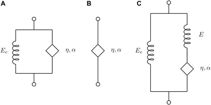
FIGURE 2. (A) Fractional Kelvin-Voigt, (B) fractional diffusion, and (C) Fractional Zener models for an order 0 < α ≤ 1.

The relaxation response of the fractional Zener model will change from dependence on an exponential, ${\mathrm{e}}^{-t/{\tau }_{\sigma }}$ to its generalization, the Mittag-Leffler function, ${\mathrm{E}}_{\alpha }[-{(t/{\tau }_{\sigma })}^{\alpha }]$. This function is defined as:

${\mathrm{E}}_{\alpha }\left(t\right)={\displaystyle \sum _{n=0}^{\infty }}\frac{t^n}{\mathrm{\Gamma }\left(\alpha n+1\right)},0<\alpha \le 1,(16)$

and it is seen that it becomes the exponential function for α = 1. The Mittag-Leffler function has power-law characteristics for large arguments, and is finite like the exponential function for small arguments.

The wave equations and asymptotes for attenuation and phase velocity for the fractional Kelvin-Voigt and fractional diffusion models shown in Figures 2A, B, will be special cases of the results to be derived in the next section.

3 Wave equation for a tempered medium model

We modify the power-law relaxation response of the fractional Kelvin-Voigt model by tempering. Tempering is a fairly common way of limiting the extent of a power-law kernel and is done by tapering it off with an exponential with time-constant τ [22, 23],:

$G\left(t\right)=E_{e}H\left(t\right)+\frac{\eta t^{-\alpha }}{\mathrm{\Gamma }\left(1-\alpha \right)}{\mathrm{e}}^{-t/\tau }.(17)$

This will limit the tail of the power-law function and thus mainly affect what happens for large time, i.e., it changes properties for low frequencies as will be evident. Other smoothly falling tempering functions could also be considered, for instance the 3-parameter Mittag-Leffler function as in [24], and which includes the exponential as a special case. Due to the shift property of the Fourier transform, an exponential is more tractable and is therefore used here, see Eqs. 22, 23.

Taking the Fourier transform gives the corresponding complex modulus:

$G\left(\omega \right)=\frac{E_e}{\mathrm{i}\omega }+\frac{\eta {\tau }^{1-\alpha }}{{\left(1+\mathrm{i}\omega \tau \right)}^{1-\alpha }},(18)$

where the second term happens to be equivalent to the complex modulus of a Cole-Davidson dielectric model of order (1 − α) [25] as pointed out in [[3], Section 8.2]. Equation 18 will be the basis for the derivation of dispersion relations and wave equations.

3.1 Tempered fractional Kelvin-Voigt model

We consider the tempered fractional Kelvin-Voigt medium and by using its Fourier transform from Eq. 18 and substituting it in Eq. 8, we obtain the dispersion relation as

$\frac{{\rho }_0{\omega }^2}{E_e}=k^2+\frac{\eta }{E_e}{\tau }^{1-\alpha }\frac{\mathrm{i}\omega }{{\left(1+\mathrm{i}\omega \tau \right)}^{1-\alpha }}{k}^2.(19)$

With $c_0^2=E_e/{\rho }_0$, the wave number can be solved for to give:

$k=\frac{\omega }{c_0}{\left[1+\frac{\eta }{E_e}{\tau }^{1-\alpha }\mathrm{i}\omega {\left(1+\mathrm{i}\omega \tau \right)}^{\alpha -1}\right]}^{-1/2}.(20)$

The asymptotic values for attenuation and phase velocity can be found using the methods of [16, 17], and Holm [3, Chap. 5]. For the different frequency regimes, the wave number can be approximated as:

$k\approx \left\{\begin{array}{cc}\frac{\omega }{c_0}{\left[\frac{\eta }{E_e}{\tau }^{1-\alpha }\mathrm{i}\omega {\left(\mathrm{i}\omega \tau \right)}^{\alpha -1}\right]}^{-1/2}=\frac{\omega }{c_0}{\left(\frac{\eta }{E_e}\right)}^{-1/2}{\left(\mathrm{i}\omega \right)}^{-\alpha /2},\hfill & \omega \tau \gg 1,\omega \eta /E_e\gg 1\hfill \\ \frac{\omega }{c_0}{\left[1+\frac{\eta }{E_e}{\tau }^{1-\alpha }\mathrm{i}\omega {\left(\mathrm{i}\omega \tau \right)}^{\alpha -1}\right]}^{-1/2}\approx \frac{\omega }{c_0}\left[1-\frac{\eta }{2E_e}{\left(\mathrm{i}\omega \right)}^{\alpha }\right],\hfill & \omega \tau \gg 1,\omega \eta /E_e\ll 1\hfill \\ \frac{\omega }{c_0}{\left[1+\frac{\eta }{E_e}{\tau }^{1-\alpha }\mathrm{i}\omega \right]}^{-1/2}\approx \frac{\omega }{c_0}\left[1-\frac{1}{2}\frac{\eta }{E_e}{\tau }^{1-\alpha }\mathrm{i}\omega \right],\hfill & \omega \tau \ll 1,\omega \eta /E_e\ll 1.\hfill \end{array}\right.(21)$

The asymptote of the negative imaginary part of the wavenumber, i.e., the attenuation of Eq. 12, follows the asymptotes of the fractional Kelvin-Voigt model for high frequencies and for the medium range (upper and middle lines in Eq. 21 respectively),

In order for the tempering to affect the lowest frequencies, the tempering time constant has to be larger than that of the spring-damper system, i.e., τ ≫ η/E. This is assumed in the approximations of Eq. 21. From the expression in the lower line of Eq. 21, it can be seen that the imaginary part of k, i.e., the attenuation, will be proportional to ω². This latter result is exactly the low frequency response of the band-limited relaxation integral of Eq. 5 with Ω_L = 1/τ, so our goal has been achieved. Likewise, from the real part of the same equation, it can be seen that for low frequencies, the phase velocity remains constant. The results are summarized in Table 2.

TABLE 2

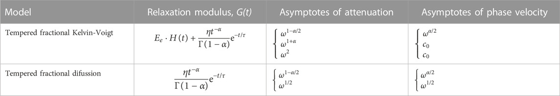
TABLE 2. Relaxation responses for t ≥ 0, and asymptotes of attenuation and of phase velocity for tempered fractional linear viscoelasticity models. Attenuation and phase velocity asymptotes are shown with the low-frequency asymptote at the bottom and the high-frequency asymptote on the top.

We now want to find the corresponding wave equation. The temporal operator corresponding to the factor (1 + iωτ)^1−α is not trivial to find, but by employing results in the dielectrics literature it can be done. The paper [26] provides a step by step derivation of the following time–frequency equivalence:

${\tau }^{\alpha -1}{\left(1+\mathrm{i}\omega \tau \right)}^{1-\alpha }\iff {\left[{\mathrm{D}}_t+1/\tau \right]}^{1-\alpha }.(22)$

Here ${\mathrm{D}}_t^{1-\alpha }$ is a standard non-integer or fractional derivative operator of order 1 − α defined by a convolution integral and ${\left[{\mathrm{D}}_t+1/\tau \right]}^{1-\alpha }$ refers to the shifted time-fractional derivative or the fractional pseudo-differential operator. The fractional pseudo-differential operator is defined as a weighted fractional derivative operator with a kernel weighted by an exponential [27, 28]:

${\left[{\mathrm{D}}_t+1/\tau \right]}^{1-\alpha }={\mathrm{e}}^{-t/\tau }{\mathrm{D}}_t^{1-\alpha }{\mathrm{e}}^{t/\tau }.(23)$

We can now derive the wave equation from Eq. 19:

${\nabla }^{2}u-\frac{1}{c_0^2}\frac{{\partial }^{2}u}{\partial t^2}+\frac{\eta }{E_e}{\left[{\mathrm{D}}_t+1/\tau \right]}^{\alpha -1}\frac{\partial }{\partial t}{\nabla }^{2}u=0.(24)$

As a test of this result the already existing power-law wave equation corresponding to the fractional Kelvin-Voigt model can be obtained as a limiting case. The fractional pseudo-differential operator can be expanded using an infinite binomial series of fractional derivatives, Garrappa et al. [28, Eq. B.18]:

${\left[{\mathrm{D}}_t+1/\tau \right]}^{1-\alpha }={\displaystyle \sum _{n=0}^{\infty }}\left(\begin{array}{c}1-\alpha \\ n\end{array}\right){\tau }^{-n}{\mathrm{D}}_t^{1-\alpha -n}.(25)$

When t/τ → 0, i.e. n = 0, this infinite series simplifies to

$\underset{t/\tau \to 0}{\lim }{\left[D_t+1/\tau \right]}^{1-\alpha }=D_t^{1-\alpha }.(26)$

Hence, in the limit we observe that the wave equation (Eq. 24) simplifies to the following:

${\nabla }^{2}u-\frac{1}{c_0^2}\frac{{\partial }^{2}u}{\partial t^2}+\frac{\eta }{E_e}\frac{{\partial }^{\alpha }}{\partial t^{\alpha }}{\nabla }^{2}u=0.(27)$

This is indeed the wave equation one would have found if one had started with the relaxation modulus of the fractional Kelvin-Voigt model as shown in, e.g., [17, 29].

3.2 Tempered fractional diffusion-wave equation

Substituting the complex modulus of Eq. 18 with E_e = 0 into Eq. 8, we obtain:

$k^2-\frac{{\rho }_0}{\eta }{\tau }^{\alpha -1}{\left(1+\mathrm{i}\omega \tau \right)}^{1-\alpha }\mathrm{i}\omega =0.(28)$

Dispersion analysis similar to that of Eq. 21 will give attenuation which increases with ω^1/2 for low frequencies and the same as for fractional diffusion for higher frequencies. Likewise the phase velocity will also vary with ω^1/2 for very low frequencies.

Using the same procedure as for the tempered fractional Kelvin-Voigt medium, we find the tempered fractional diffusion-wave equation:

${\nabla }^{2}u-\frac{{\rho }_0}{\eta }{\left[{\mathrm{D}}_t+1/\tau \right]}^{1-\alpha }\frac{\partial u}{\partial t}=0.(29)$

This is equivalent to the tempered fractional diffusion wave equation of, e.g., [30] (Section 2.2), that can describe a transition from an anomalous sub-diffusion regime to the normal diffusion regime. The relaxation response of the tempered fractional diffusion wave equation has been used to model the responses of elastomers, Polydimethylsiloxane (PDMS), and the rheological behavior of alginate-based gels [31].

Using the same limiting operation for τ → ∞ as in the previous section, we observe that the wave equation (Eq. 29) simplifies to the following:

${\nabla }^{2}u-\frac{{\rho }_0}{\eta }\frac{{\partial }^{2-\alpha }u}{\partial t^{2-\alpha }}=0.(30)$

This is the fractional diffusion-wave equation.

The properties of the tempered Kelvin-Voigt and diffusion models are summarized in Table 2.

4 Discussion

There exist numerical schemes for fractional derivative equations in general [32] as well as for the fractional pseudo-differential operator of Eq. 23, e.g., the diffusive representation of [33].

The fractional diffusion-wave equation (Eq. 30), has been analyzed extensively. The Green’s function, the generalization of Eq. 14, is given in [[34], Eq. 9]. They also comment that their time-space solution “can be used to give a new proof of the known fact that …a response of the time-fractional diffusion–wave equation …to a localized disturbance spreads infinitely fast.” They also shows that the maximum in time occurs at a time proportional to x^2/(2−α), Luchko et al. [34, Eq. 16].

Relaxation responses of the form of Eq. 17 have some similarity with the compressional and shear wave models of the Viscous Grain-Shearing model for sediment acoustics. The derivation is however very different as [35] starts with time-varying models to get the relevant relaxation responses. There are also changes in constants and terminology, as well as an additional independent power-law term in Eq. 17 in that work. As fractional calculus is not used in that work, the wave equations formulated as in Eqs. 24, 29, are not found there.

In the case of a fit to a lower frequency limit of, for example, 2 kHz as in the sediment acoustics example of Williams et al. [13, Figure 6] mentioned earlier, the time constant of the tempering would be in the order of τ = 1/(2π ⋅ 2000) ≈ 0.08 ms. This value is comparable to the value of 0.12 ms used for what is called the viscoelastic time constant in Buckingham [35, Table 1].

The tempered models considered here both have relaxation responses with an initial singularity. Although we have argued that the resulting initial transient that travels with infinite velocity is negligible, it may be desirable with a model that avoids it completely. This can be achieved by tempering the non-singular relaxation response of the fractional Zener model, i.e., by multiplying the Mittag-Leffler function in the lower left corner of Table 1 with an exponential. Its Laplace transform is given in [24] and it is possible to find the corresponding wave equation. It will have a total of five terms including three loss terms, one more loss term than that of the fractional Zener model. The fractional Maxwell model also avoids the singularity at t = 0. Its relaxation response is similar to that of the fractional Zener model, but without the constant term. As the Maxwell model is primarily relevant for fluid media, it will not be considered here.

An alternative way for tempering the fractional Zener model is to start with the four-term wave equation for the fractional Zener model. It is similar to that for the fractional Kelvin-Voigt model in Eq. 27 but with the addition of a loss term with temporal derivative order α + 2 [16]. One may substitute all the fractional derivatives with fractional pseudo-differential operators, similar to when moving from Eq. 27 to Eq. 24. The relaxation response which corresponds to this new wave equation can then be found, but G(t) only can be expressed as an infinite series as in [24]. Such a tempered fractional Zener wave equation is also relevant for modeling acoustic wave propagation in marine sediments. In [26], it was shown that the shear wave mode and the fast compressional wave mode of the Biot poroelastic model can be described by tempered half-order fractional Zener models.

In our view, the added complexity of either of these approaches for finding a tempered non-singular kernel based on the fractional Zener model outweighs the advantages, so further results are therefore not given here.

5 Conclusion

The goal of this paper was to modify the fractional Kelvin-Voigt and fractional diffusion medium models in order make the variation with frequency at low frequencies more steep. This was patterned after the ω² behavior of a truncated sum of relaxation processes below the lower frequency limit. We found that tempering of the relaxation modulus with an exponential would lead to such behavior for the fractional Kelvin-Voigt model. In the case of the fractional diffusion model, it led to $\sqrt{\omega }$ behavior below the low frequency limit. Both of these models are used for modeling compressional and shear waves in sediment acoustics, but in these cases they are formulated without fractional derivatives as done in the current work.

The wave equations for the tempered models were found by employing the fractional pseudo-differential operator, as is also done in analysis of the Cole-Davidson model for dielectrics. The tempered power-law wave equations are equivalent to equations discussed in the fractional calculus literature and this makes it possible to draw on already existing literature for analysis of the properties of the solutions, like the effect of the singularity in the relaxation modulus of these models.

Data availability statement

The original contributions presented in the study are included in the article. Further inquiries can be directed to the corresponding author.

Author contributions

SH: initiated the project, conceptualization and writing of the original draft, SC: development of main equations of Section 3 and validation, SN: conceptualization and validation. All authors contributed to the article and approved the submitted version.

Funding

This work was supported by the Research Council of Norway under Grant No. 237887, Centre for Innovative Ultrasound Solutions.

Conflict of interest

The authors declare that the research was conducted in the absence of any commercial or financial relationships that could be construed as a potential conflict of interest.

Publisher’s note

All claims expressed in this article are solely those of the authors and do not necessarily represent those of their affiliated organizations, or those of the publisher, the editors and the reviewers. Any product that may be evaluated in this article, or claim that may be made by its manufacturer, is not guaranteed or endorsed by the publisher.

References

1. Szabo TL, Wu J. A model for longitudinal and shear wave propagation in viscoelastic media. J Acoust Soc Am (2000) 107:2437–46. doi:10.1121/1.428630

PubMed Abstract | CrossRef Full Text | Google Scholar

2. Mainardi F. Fractional calculus and waves in linear viscoelesticity: An introduction to mathematical models. London, UK: Imperial College Press (2010). doi:10.1142/p614

CrossRef Full Text | Google Scholar

3. Holm S. Waves with power-law attenuation. Switzerland: Springer and ASA Press (2019). doi:10.1007/978-3-030-14927-7

CrossRef Full Text | Google Scholar

4. Zhao X, McGough RJ. Time-domain comparisons of power law attenuation in causal and noncausal time-fractional wave equations. J Acoust Soc Am (2016) 139:3021–31. doi:10.1121/1.4949539

PubMed Abstract | CrossRef Full Text | Google Scholar

5. Parker K, Szabo T, Holm S. Towards a consensus on rheological models for elastography in soft tissues. Phys Med Biol (2019) 64:215012. doi:10.1088/1361-6560/ab453d

PubMed Abstract | CrossRef Full Text | Google Scholar

6. Holm S, Holm MB. Restrictions on wave equations for passive media. J Acoust Soc Am (2017) 142:1888–96. doi:10.1121/1.5006059

PubMed Abstract | CrossRef Full Text | Google Scholar

7. Van Moll CAM, Ainslie MA, Van Vossen R. A simple and accurate formula for the absorption of sound in seawater. IEEE J Oceanic Eng (2009) 34:610–6. doi:10.1109/joe.2009.2027800

CrossRef Full Text | Google Scholar

8. Näsholm SP, Holm S. Linking multiple relaxation, power-law attenuation, and fractional wave equations. J Acoust Soc Am (2011) 130:3038–45. doi:10.1121/1.3641457

PubMed Abstract | CrossRef Full Text | Google Scholar

9. Näsholm SP. Model-based discrete relaxation process representation of band-limited power-law attenuation. J Acoust Soc Am (2013) 133:1742–50. doi:10.1121/1.4789001

PubMed Abstract | CrossRef Full Text | Google Scholar

10. Pierce AD, Mast TD. Acoustic propagation in a medium with spatially distributed relaxation processes and a possible explanation of a frequency power law attenuation. J Theor Comp Acoust (2021) 29:2150012. doi:10.1142/s2591728521500122

CrossRef Full Text | Google Scholar

11. Gradshteyn IS, Ryzhik IM. In: YV Geronimus, and MY Tseytlin, editors. Table of integrals, series, and products. United States: Academic Press (2014).

Google Scholar

12. Futterman WI. Dispersive body waves. J Geophys Res (1962) 67:5279–91. doi:10.1029/jz067i013p05279

CrossRef Full Text | Google Scholar

13. Williams KL, Jackson DR, Thorsos EI, Tang D, Schock SG. Comparison of sound speed and attenuation measured in a sandy sediment to predictions based on the biot theory of porous media. IEEE J Ocean Eng (2002) 27:413–28. doi:10.1109/joe.2002.1040928

CrossRef Full Text | Google Scholar

14. Hall L. The origin of ultrasonic absorption in water. Phys Rev (1948) 73:775–81. doi:10.1103/physrev.73.775

CrossRef Full Text | Google Scholar

15. Tschoegl NW. The phenomenological theory of linear viscoelastic behavior: An introduction. Berlin: Springer-Verlag (1989). Reprinted in 2012.

Google Scholar

16. Holm S, Näsholm SP. A causal and fractional all-frequency wave equation for lossy media. J Acoust Soc Am (2011) 130:2195–202. doi:10.1121/1.3631626

PubMed Abstract | CrossRef Full Text | Google Scholar

17. Holm S, Sinkus R. A unifying fractional wave equation for compressional and shear waves. J Acoust Soc Am (2010) 127:542–8. doi:10.1121/1.3268508

PubMed Abstract | CrossRef Full Text | Google Scholar

18. Fichera G. Is the Fourier theory of heat propagation paradoxical? Rendiconti Del Circolo Matematico di Palermo (1992) 41:5–28. doi:10.1007/bf02844459

CrossRef Full Text | Google Scholar

19. Awad E. On the time-fractional Cattaneo equation of distributed order. Physica A: Stat Mech Appl (2019) 518:210–33. doi:10.1016/j.physa.2018.12.005

CrossRef Full Text | Google Scholar

20. Maxwell JC. Theory of heat, II. Harlow, United Kingdom: Longmans, Green & Co (1972).

Google Scholar

21. Mainardi F. Fractional calculus and waves in linear viscoelesticity: An introduction to mathematical models. 2nd ed. London, UK: World Scientific (2022). doi:10.1142/p614

CrossRef Full Text | Google Scholar

22. Cartea Á, del Castillo-Negrete D. Fluid limit of the continuous-time random walk with general Lévy jump distribution functions. Phys Rev E (2007) 76:041105. doi:10.1103/physreve.76.041105

PubMed Abstract | CrossRef Full Text | Google Scholar

23. Pandey V, Näsholm SP, Holm S. Spatial dispersion of elastic waves in a bar characterized by tempered nonlocal elasticity. Fract Calc Appl Anal (2016) 19:498–515. doi:10.1515/fca-2016-0026

CrossRef Full Text | Google Scholar

24. Liemert A, Sandev T, Kantz H. Generalized Langevin equation with tempered memory kernel. Phys A: Stat Mech Applic (2017) 466:356–69. doi:10.1016/j.physa.2016.09.018

CrossRef Full Text | Google Scholar

25. Davidson D, Cole RH. Dielectric relaxation in glycerine. J Chem Phys (1950) 18:1417. doi:10.1063/1.1747496

CrossRef Full Text | Google Scholar

26. Chandrasekaran SN, Näsholm SP, Holm S. Wave equations for porous media described by the Biot model. J Acoust Soc Am (2022) 151:2576–86. doi:10.1121/10.0010164

PubMed Abstract | CrossRef Full Text | Google Scholar

27. Nigmatullin R, Ryabov YE. Cole–Davidson dielectric relaxation as a self-similar relaxation process. Phys Solid State (1997) 39:87–90. doi:10.1134/1.1129804

CrossRef Full Text | Google Scholar

28. Garrappa R, Mainardi F, Maione G. Models of dielectric relaxation based on completely monotone functions. Fract Calc Appl Anal (2016) 19:1105–60. doi:10.1515/fca-2016-0060

CrossRef Full Text | Google Scholar

29. Pandey V, Holm S. Connecting the grain-shearing mechanism of wave propagation in marine sediments to fractional order wave equations. J Acoust Soc Am (2016) 140:4225–36. doi:10.1121/1.4971289

PubMed Abstract | CrossRef Full Text | Google Scholar

30. Sandev T, Sokolov IM, Metzler R, Chechkin A. Beyond monofractional kinetics. Chaos Solit Fractals (2017) 102:210–7. doi:10.1016/j.chaos.2017.05.001

CrossRef Full Text | Google Scholar

31. Bonfanti A, Kaplan JL, Charras G, Kabla A. Fractional viscoelastic models for power-law materials. Soft Matter (2020) 16:6002–20. doi:10.1039/d0sm00354a

PubMed Abstract | CrossRef Full Text | Google Scholar

32. Diethelm K, Garrappa R, Stynes M. Good (and not so good) practices in computational methods for fractional calculus. Mathematics (2020) 8:324. doi:10.3390/math8030324

CrossRef Full Text | Google Scholar

33. Blanc E, Chiavassa G, Lombard B. A time-domain numerical modeling of two-dimensional wave propagation in porous media with frequency-dependent dynamic permeability. J Acoust Soc Am (2013) 134:4610–23. doi:10.1121/1.4824832

PubMed Abstract | CrossRef Full Text | Google Scholar

34. Luchko Y, Mainardi F, Povstenko Y. Propagation speed of the maximum of the fundamental solution to the fractional diffusion–wave equation. Comput Math Appl (2013) 66:774–84. doi:10.1016/j.camwa.2013.01.005

CrossRef Full Text | Google Scholar

35. Buckingham MJ. On pore-fluid viscosity and the wave properties of saturated granular materials including marine sediments. J Acoust Soc Am (2007) 122:1486–501. doi:10.1121/1.2759167

PubMed Abstract | CrossRef Full Text | Google Scholar