- School of Statistics and Mathematics, Shandong University of Finance and Economics, Jinan, China
Topological data analysis has been acknowledged as one of the most successful mathematical data analytic methodologies in many fields. Additionally, it has also been gradually applied in financial time series analysis and proved effective in exploring the topological features of such data. We select 100 stocks from China’s markets and construct point cloud data for topological data analysis. We detect critical dates from the Lp-norms of the persistence landscapes. Our results reveal the dates are highly consistent with the transition time of some major events in the sample period. We compare the correlations and statistical properties of stocks before and during the events via complex networks to describe the markets’ situation. The strength and variation of links among stocks are clearly different during the major events. We also investigate the neighborhood features of stocks from topological perspectives. This helps identify the important stocks and explore their situations under each event. Finally, we cluster the stocks based on the neighborhood features, which exhibit the heterogeneity impact on stocks of the different events. Our work demonstrates that topological data analysis has strong applicability in the dynamic correlations of stocks.
1 Introduction
In recent years, major public events have frequently occurred, and they can easily bring substantial and negative impacts to the financial markets, leading to dramatic fluctuations in stock prices. For example, the coronavirus disease 2019 (COVID-19) has swept across the world, rapidly spreading to more than 200 countries and becoming a global public health and economic catastrophe [1]. Under such situations, people are more cautious about investing, resulting in a significant decrease in market liquidity [2]. Tracking the dynamic market changes and identifying critical information is vital to prevent systemic financial risks. Various methods and models have been applied to help identify the risks or identify early warning signals.
Before 2008, the early warning indicator method was one of the most common for measuring systemic financial risks, being simple, clear, practical, and effective. However, it only investigates static conditions of financial systems. The risk contagion effect, negative external characteristics, and system correlations remain unknown under this method [3]. The composite index method significantly compensates for this deficiency, helping to dynamically reflect the comprehensive situation of the risks of the financial system. However, the various indicator levels are all artificially weighted, which separates the dynamic evolution process and inevitably generates prediction errors. After the advent of the 2008 global financial crisis, scholars began to pay more attention to the correlations and contagions of risks within the financial systems, and financial risk spillover indices were widely used [4, 5]. The related models and methods were gradually enriched [6–10]. Recently, multiple models have been commonly used to comprehensively consider financial risk [11, 12]. However, most of these studies often use a representative stock index for each country. For example, the CSI 300 Index is most commonly used in China. Most studies directly use the stock indices to measure risks [13, 14]. However, the indices cannot describe the changes in the stocks’ internal structures more comprehensively and accurately. The components of the CSI 300 Index are adjusted every 6 months in principle, and the weights are calculated based on the free float. Although the weights change dynamically, it is not easy to extract the internal structure of relatively similar stocks. For example, if two components of a stock index have exactly the same weighting, and if the rise of one is exactly as great as that of the other, then the change in the index is hardly captured. Therefore, we focus on China’s markets and attempt to identify a new indicator that can accurately portray the dynamic evolution of financial risks and effectively capture the risk changes in the financial system under major events. This indicator can help obtain early warning signals of systemic risks in China’s stock market.
We apply topological data analysis (TDA) by constructing point clouds data of stock returns over the past 20 years and calculating Lp-norms of the persistence landscapes of the data to obtain a new indicator with a topological perspective. TDA provides an increasing number of methods to explore topological features of multifarious data [15, 16], especially for big data. Carlsson [16] systematically introduces the theoretical basis of simple homology, persistent homology, and complex shape; among which, the advantage of persistent homology is that it can accurately describe the whole picture of the data without dimension reduction and exhibit key topological features such as the number of clusters and ring structures in the data. Bubenik [17] adds the concept of persistent landscapes to provide reasonable quantification of persistent homology. Furthermore, the construction of the persistence landscapes toolbox [18] provided important support for the application. In their investigation of financial markets based on persistent landscapes, Gidea [19] documents that Lp-norms display a significant trend during market crashes. Guo et al. [20] demonstrate that TDA works well in analyzing financial crises. With the continuous deepening of research, topology is gradually becoming widely used in financial markets [21, 22]. Therefore, we conduct TDA on stocks chosen from China’s market to investigate topological features, especially situations before and during a major public event. We identify the critical dates when Lp-norms decline significantly, which indicates an obvious increase in the stocks’ overall correlations. We then construct complex networks for individual stocks to provide reasonable explanations of correlations within the stock market. We derive the neighborhood norms for each stock and use K-means to cluster the stocks. We also compare the changes in the classification of individual stocks before and after the critical dates.
The procedure implemented in this study is illustrated in Figure 1. We use TDA to analyze the topological features of the stocks from a new perspective and provide new indicators to capture the critical changes in the data. We creatively select 30 stocks with the highest correlations of each stock as its neighborhood(s) and calculate the Lp-norms of every such clique to investigate the neighborhood feature(s) of each stock, which can reflect the position and importance of each stock among the whole. We consider the norm as a higher-order attribute for each stock and cluster them accordingly. We then comprehensively analyze the dynamic evolution of the correlations among stocks in various industries during major public events.

FIGURE 1. Flowchart of the procedure implemented. There are two parts. The first part involves data collection, processing, and point cloud construction. The second concerns TDA-related computations and empirical study.
2 Materials and methods
2.1 Data collection and processing
We focus our research on China’s stock markets. First, according to the latest Standard Industrial Classification (SIC system), we randomly selected 150 A-share stocks in various industries and collected the closing prices of Shanghai and Shenzhen A-share component stocks between 2005/01/01 and 2022/03/31 from the Wind Financial Database. Considering factors such as long-term suspension and delisting, we cleaned the data and derived a sample of 100 stocks to examine their performance in terms of various stock market indicators during typical major events in the sample period.
There is a small amount of missing data among the daily closing price series of stocks. We interpolate the closing price and finally obtain that of 4,189 trading days. We use their daily log returns; that is, ri(t) = lnPi(t) − lnPi(t − 1), i ∈ 1, 2, …, 100, where Pi(t) is the closing price of the index on trading day t.
We applied the sliding window method to process the data as follows. For each trading day t, we selected the daily return series (ri(t − ω + 1), ri(t − ω + 2), …, ri(t)) and (rj(t − ω + 1), rj(t − ω + 2), …, rj(t)) for each pair of stocks (i, j) based on the sliding window size ω (i.e., from trading day t − ω + 1 to trading day t). We then obtained the corresponding correlation coefficients Ct(i, j) and transformed into the distance measure dt(i, j) using
2.2 Background of TDA
2.2.1 Persistent homology
To better understand persistent homology, imagine that we have a point cloud. Furthermore, suppose there is a parameter that defines the radius of a ball centered on each data point, and as the parameter increases, each ball gradually comes into contact with the other balls. These processes of ball contact enable the emergence of unique topological features, thus providing a new perspective on financial time series and other data. TDA is constructed as a filter of complex shapes while calculating persistent homology with the point cloud data to sort a certain resolution parameter. It is characterized by the fact that the data is not only retained in the original high-dimensional space, but also the number of clusters and ring structures present is identified, and the whole process does not require visualization of the data.
2.2.2 Simplicial complexes
A simplex is defined on a finite vertex set. For example, a k-simplex is a polyhedron with k + 1 vertices and k + 1 faces. A simplicial complex K is a set of simplexes and satisfies the following two conditions: (1) Any face of any simplex in K still belongs to K. (2) The intersection of any two simplexes κ1, κ2 in K is either the empty set or one of the common surfaces of both. The most common simplicial complexes are Vietoris—Rips, Čech, witness, and Alpha complexes, among others. We use the Vietoris-Rips complexes because these approximate the more exact Čech complexes but are more efficient to calculate [22].
Suppose we have a point cloud A = {x1, x2, …, xn} in a topological space X endowed with a metric d. Denote the ɛ-ball of each point x ∈ X by Bɛ = {y ∈ X: d(y, x) < ɛ, y ≠ x} for any ɛ > 0. A Vietoris–Rips complex VR(A, ɛ) w.r.t the positive value ɛ is the simplicial complex whose vertices set is A and where
2.2.3 Barcodes and persistence diagrams
The persistence barcode is the most direct way to characterize a complex and quantify its change with the increasing value ɛ. A barcode [24] is a graphical representation of a collection of horizontal line segments {Ij: j ∈ J} in a plane with each interval as the life of a topological hole, that is, a homology class. For example, an interval Ij = [aj, bj] in a 0-dim barcode corresponds to a connected component in the complex with the meaning that the component emerges when ɛ = aj and vanishes when ɛ = bj; an interval in a 1-dim barcode corresponds to an independent loop in the complex with the endpoints as the value when the loop emerges and vanishes. However, it is not sufficient to analyze the shape of the data only by the barcodes; we need other ways to convert the barcodes to computable properties. A natural representation of a barcode called a persistence diagram (see Cohen-Steiner et al. [25]) is the set {(aj, bj): j ∈ J}. Note that each (aj, bj) here is a 2-dim point, where aj and bj are the endpoints of the interval Ij in the barcode. We can compare and calculate the difference between the diagrams by bottleneck distance and degree p Wasserstein distance (see Cohen-Steiner et al. [25], Gidea and Katz [19], respectively). They induce a metric on the space of persistence diagrams.
2.2.4 Persistence landscapes and Lp-norms
To grasp the continual change of the data shapes, persistence landscapes, and their Lp-norms introduced in Bubenik [17] improve the method effectively. Applying them to the complexes, we can observe the shapes’ continual change of the point cloud data. Furthermore, persistence landscapes maintain robustness as diagrams under perturbations of the data. Briefly, the persistent landscapes are the piecewise functions corresponding to any point (aj, bj) in the persistent graph as follows,
Then, we define
where kmax denotes the k-th largest element for
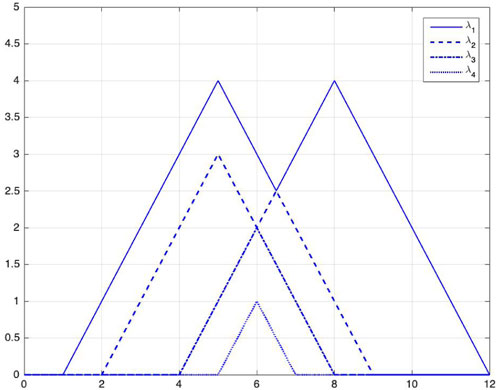
FIGURE 2. Persistence landscapes of an example, i.e., images of the functions λ1, λ2, λ3, and λ4 from top to bottom. We calculate them using Eqs 1, 2. The critical points of the persistence landscape
Persistence landscapes form a subset of the Banach space
where
2.3 Background and topological measures of complex networks
To establish a threshold network, we first construct an adjacency matrix A = (A(u, v)) based on the distance matrix D = (d(u, v)). When d(u, v) is less than or equal to a given threshold θ, the corresponding element A(u, v) = 1 in the adjacency matrix, and then the vertices u and v are connected by an edge (also called correlated); otherwise, A(u, v) = 0, and thus there is no edge connecting u and v directly. Considering the importance of the adjacency matrix, we present its definition below,
Note that the edges in the network have neither direction nor weight, and we refer to it as a non-directional and unweighted network. Such a complex network constructed in the above way is called a threshold network. To observe the features of such networks, we introduce four topological properties, including degree, density, clustering coefficient, and average path length.
Suppose the network contains N vertices. The degree of a vertex u is the number of edges connected to that vertex. The average degree of a network is the average of degrees for all vertices in the network [26], referred to as the degree of the network. Denote by M the actual number of edges. The maximum possible number of edges is obviously
Denote by ku the degree of the vertex u, that is, there are ku vertices connecting the vertex u. Eu is the number of edges between these ku vertices. The clustering coefficient of vertex u, denoted by Cu, is then defined in the following way when ku ≥ 2,
When ku is equal to 0 or 1, the clustering coefficient Cu of vertex u is specified as 0. The clustering coefficient of the network is the average clustering coefficient of all vertices in the network, that is,
In the network, the number of edges contained in the shortest path from the vertex u to the vertex v is referred to as the shortest path length between u and v, denoted by Duv. The average path length of the network, denoted by L, is defined as the average of the shortest path length between each pair of vertices in the network, that is,
By the definitions of the above four topological properties, we know that the larger they are, the closer the vertices in the network are connected, except for the average path length. By contrast, for the average path length of a network, the smaller it is, the more closely the vertices are connected.
2.4 K-means clustering algorithm and elbow method
Suppose that data can be divided into K classes (K is known). The data are a set of n observations, that is, {x1, …, xn}. The observations are divided into K non-intersecting sets {C1, …, CK}, and all clusters are concatenated for the whole sample. i ∈ Ck means that the i-th observation xi belongs to the k-th cluster. We want the “in-group variation” of each cluster to be as small as possible, and the mean or center position of cluster k is given by:
where |Ck| denotes the number of observations in cluster k. There are K means in the sample, so we refer to the algorithm as K-means clustering. For an observation xi(i ∈ Ck) in cluster k, the deviation (xi − ck) from the center of the cluster is called the “error.” The sum of squares of all the errors in cluster k is the sum of squares error (SSE) of cluster k:
where ‖xi − ck‖ is the Euclidean distance. The SSE of all clusters is summed to obtain the SSE of the full sample; the objective is to find a division C1, …, CK for the set of sample subscripts 1, …, n that minimizes the SSE of:
Because it is difficult to determine the global minimum solution to the problem, K-means clustering generally uses an iterative algorithm to find the local minimum solution. The results obtained will depend on the initial (random) cluster assignment of each observation. For this reason, it is important to run the algorithm multiple times from different random initial configurations. Another key issue in using K-means clustering is how the number of clusters K should be chosen.
The elbow method as a heuristic is a commonly used cluster analysis method, which helps determine the optimum number K of clusters. The method can improve the accuracy and reliability of cluster analysis. The basic principle of the elbow method is to determine the optimal number of clusters by calculating the sum of SSE for different numbers of clusters. When the number of clusters increases, the SSE decreases, but the rate of decrease slows. When the number of clusters increases to a certain point, the decrease in SSE slows rapidly, forming an elbow. This elbow is the key to the K-means elbow rule, which indicates the optimal number of clusters.
3 TDA-based systemic financial risk analysis
3.1 Construction of point clouds data and persistence landscapes
For each trading day t, we consider all stocks as points to construct the point cloud data and carry out TDA on the complexes, mainly based on the persistence landscapes. We consider the 0- and 1-dim barcodes and calculate the Lp-norms of the persistence landscapes both together. We first choose the length of the sliding window to obtain reasonable parameters for subsequent analysis. After comparison, the Lp-norms clearly exhibit better results with a sliding window ω = 100.
In Figure 3, we present an overall description of 100 stocks and want to compare the general indicators with the Lp-norms to illustrate the significance of using the TDA measure. We plot the average of 100 stocks’ return series and the average of their standard deviations in Figures 3A,B, respectively. The standard deviation, a common method for calculating volatility, measures the degree of volatility of a particular return series. Thus, the average standard deviation of the 100 stocks in Figure 3B can approximately depict the state of our stock market and also capture the turbulence in the market (manifested as an increase in the standard deviation).

FIGURE 3. Common indicators and corresponding norms series of the 100 stocks over the full sample period. (A) Average daily log returns of 100 stocks. (B) Average standard deviations of 100 stocks. Our aim is to document the fluctuations of the market approximately. (C) L1- and L2-norms of persistent landscapes are calculated using both 0- and 1-dim barcodes; the period is from 2005/06/09 to 2022/03/31.
The L1-and L2-norms of persistence landscapes of the point cloud data are depicted in Figure 3C. In detail, the norms are based on the simplicial complex of high-dimensional point clouds, so the values of the norms are closely related to the distances and the structures of the point clouds. The smaller the norms correspond, the closer the distances; that is, the stronger the correlation between the stocks. We can observe the following phenomenon. Compared to the norms we obtained, the valleys of the norms are significantly less than the peaks of the standard deviation. This is because if the log return persists at a high level of volatility for a long period, its corresponding norms are small. Conversely, if the log return is very high in volatility at a time point or sits at a high level of volatility for a short period, its corresponding norms are at normal levels. This illustrates that the norms calculated from the topological perspective are very robust to outliers.
Obviously, the L1-and L2-norms were low and recovering from 2005, influenced by the SARS epidemic in 2003. Beginning at the end of October 2007, the return fluctuated rapidly and sharply, and the norms hit bottom in 2008 owing to the U.S. Subprime Lending Crisis along with the Wenchuan earthquake in China. The standard deviation continued to be at a high level for a long period of time and the L1-and L2-norms declined significantly. The link among the stocks became closer, and the situation was severe. From December 2014 to May 2015, there was a fast-rising bull market in China’s stock market, during which the Shanghai and Shenzhen stock indices rose in turn (the Shanghai Composite Index and Shenzhen Stock Index accumulated 53.17% and 57.13%, respectively). Subsequently, the China Securities Regulatory Commission began to rectify illegal allocation and forced deleveraging in the short term, leading to a continuous decline in the A-share market. From June to September, the Shanghai Composite Index cumulatively declined −42.26% and the Shenzhen Composite Index declined −48.74%. The standard deviation rose to a record peak. This, in turn, led to successive plunges in various stock market-style assets. Hence, China’s 2015 stock market crash led to an unstable economic situation, and the norms rapidly fell to record valleys. The connections among stocks became increasingly close during the crisis period. Since 2018, China’s stock market has no longer been stable and flat due to the trade war between China and the U.S. and the COVID-19 pandemic. In general, when major events occur, the average standard deviation rises gradually. L1-and L2-norms exhibit obvious drops and are at a low level, indicating that the structure of the data changes and the connections among stocks becomes close. Whenever there is a sudden structural change, our persistence landscapes change. This leads to changes in Lp-norms. This is especially evident when the structure shifts to tighter situations. The use of persistence landscapes and Lp-norms as barometers of shocks enables timely information to be detected.
3.2 Critical dates detection and analysis
We want to extract the feature of the returns using the aforementioned data processing method. Guo et al. [20] used TDA and detected the early warning signal of the 2008 crisis in the first half of 2007. The TDA model provides a better definition of market signals, especially during financial meltdown cycles [21]. The trend of the L1-norms is similar to that of L2-norms, but the L1-norms change more frequently. We predict that using the L1-norms can detect more critical dates than the L2-norms with the same other parameters and validate it through multiple tests.
We built a system to detect dates with sharp changes in point cloud data by referring to Guo et al. [20]. For every trading day t, we calculated and denoted by N(t) the Lp-norms of the persistence landscape of the complex (we calculated the Lp-norms of trading day t based on the sliding window from the point cloud data of trading day t − ω + 1 to trading day t), and by A(t) the Lp-norms’ mean value of m consecutive trading days before day t. If the following two conditions are satisfied, we take trading day t as the critical date for a financial crisis or risk: i) The ratio N(t)/N(t − 1) ≤ α for a fixed α < 1. ii) The ratio N(t)/A(t) ≤ β for a fixed β < 1. For simplicity, let m = 100.
The first condition indicates the presence of risk on trading day t, whereas the second ensures that it is a true crisis-critical date. It is possible to identify multiple dates, which indicate significant stock market shocks, but some may be only brief declines caused by coincidental events that are not representative. Under the L1-and L2-norms, some of the critical dates detected for the parameters at different values are list in Table 1.
From Table 1, the highest number of critical dates were detected for 2007–2008, with 2008/04/02 and 2008/06/10 appearing most frequently, followed by critical dates detected under different combinations of parameters for 2015 (2015/08/20, 2015/08/28, and 2015/11/02). The critical date in 2018 is 2018/12/03, those in 2020 are 2020/02/03 and 2020/04/01, and for 2022 is 2022/03/29. Considering that some events last longer and even had multiple rounds of shocks, we used the first identified dates in the critical years as representative critical dates for comparability: 2008/04/02, 2015/08/20, 2018/12/03, 2020/02/03,4 and 2022/03/29.
We use the same method to obtain the log return of the CSI 300 Index. Using the financial crisis-critical date detection system for its log returns, there are many sudden change dates, and it does not focus on identifying the real crisis-critical dates. In contrast, the norm series can better focus on and capture the critical dates of a real crisis, so it will be more effective to use this to perform region transformation in the future.
We analyze the stocks’ relevance for all critical dates and the 50th days before. To save space, Figure 4A–D present only the persistent landscapes composed of point clouds before and at the time of two major events, depicting the evolution of data shapes before and during each critical date. Two endpoints of the intersection of each layer with the horizontal axis correspond to the left and right endpoints of each interval of the 1-dim barcode, respectively. The highest layer corresponds to the longest interval of the barcode. The comparison indicates different degrees of change in persistent landscapes before and after the first outbreak of the two events. Those in Figure 4B tend to become smaller in most triangles compared with those in Figure 4A; that is, the norms are significantly lower. Compared to Figure 4C, the persistent landscapes in Figure 4D exhibit a significant decrease in the highest layer, and the right side of the triangle is no longer concentrated in 0.6–1.1 but is more scattered in 0.4–1, thus limiting the total area of the inner layers to decrease. This reflects the decrease in the norm. Moreover, pre-crisis to crisis norms decrease more. We obtain good evidence that the stock market links strengthen when a crisis occurs.
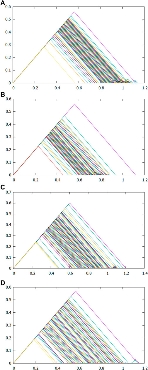
FIGURE 4. Persistent landscapes on 2008/01/16, 2008/04/02, 2019/11/14, and 2020/02/03 from (A–D), respectively. The figures contain many
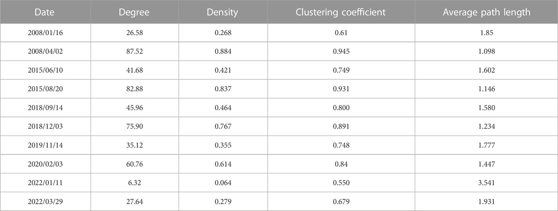
We plotted threshold networks for each of the five pairs of critical dates identified. To obtain a reasonably uniform threshold θ, we calculated and compared the degrees of networks of the 10 aforementioned dates, and separately differed the degrees of networks of the critical dates from their corresponding previous 50th days. When θ = 1.1, the average difference of the network average degrees for the five pairs of critical dates reaches the maximum level. The comparison of the topological indicators of the return threshold network is presented in Table 2. Our stock market moved the most during the financial crisis triggered by the U.S. Subprime Lending Crisis in 2008 and the stock market crash in 2015, followed by the trade war between China and the U.S. in 2018 and the COVID-19 pandemic in 2020 and 2022. Before and after the U.S. Subprime Lending Crisis in 2008 and the stock market crash in 2015, the degree of the network increased from 26.58 to 41.68 to 87.52 and 82.88, the network density increased from 0.268 to 0.421 to 0.884 and 0.837, the clustering coefficient of the network changed from 0.61 to 0.749 to 0.945 and 0.931, and the average path length of the network from 1.85 to 1.602 to 1.098 and 1.146, respectively. Hence, the connection between stocks became stronger. The return threshold networks for 2015/06/10 and 2015/08/20 are presented in Figure 5. The number of connected edges in the network increases significantly before and after the event, indicating that the stock market is closely linked under major event shocks. This result is consistent with previous findings.
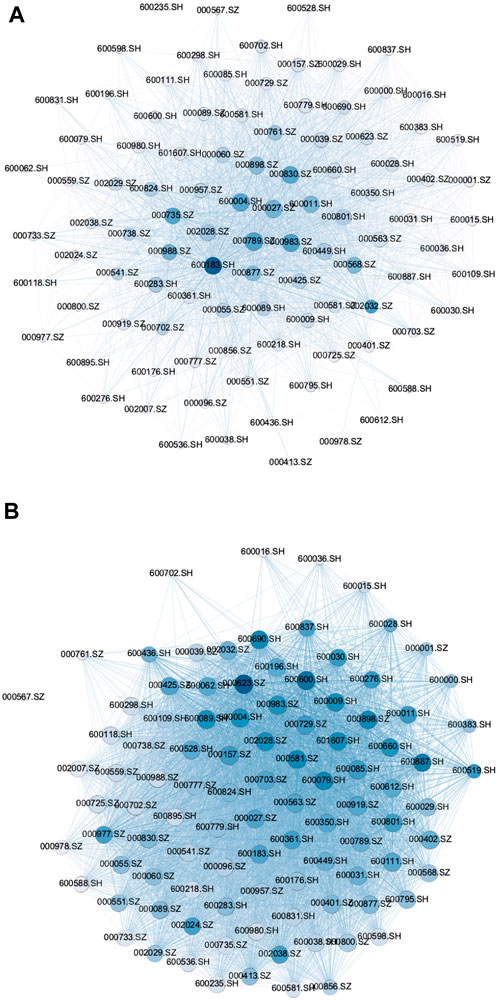
FIGURE 5. Comparison of the return networks for 2015/06/10 and 2015/08/20. For example, in 2015, we find a significant increase in the number of connected edges in the network when an event occurs. (A) Return network on 2015/06/10. (B) Return network on 2015/08/20.
The correlation coefficients and corresponding frequent dynamic distribution, calculated from the daily log returns with a rolling window of 100 trading days, are illustrated in Figure 6. The correlation coefficients among stocks at normal times are mostly distributed in the interval of −0.25 to 0.50, and the corresponding probability distributions are between 0 and 0.1, which are approximately normal. This indicates that the correlations among stocks are not significant, and the clustering effect is not obvious. However, the peaks of the cross-sectional graphs of the frequency distribution of correlation coefficients in 2008 and 2015 are higher. Therefore, we think the correlation coefficients among stocks generally tend to rise and cluster during a sudden event. The changes in 2018 and 2020 are smaller than the previous two systemic risks, confirming that differences exist in the degree of impact of each major event on China. The following section analyzes the evolution of heterogeneity in the structure of the stock market under different events using the higher-order characteristics of stocks (i.e., neighborhoods).
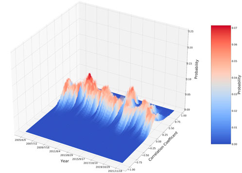
FIGURE 6. Correlation coefficients and corresponding frequent dynamic distribution of 100 stocks. The lateral axis represents time, the longitudinal axis represents the correlation coefficient values, and the vertical axis represents the frequency of the correlation coefficients appearing in a certain interval at a specific time point.
4 Comparison and mechanisms of neighborhood norms before and during the events
4.1 Overall neighborhood norms and their applications
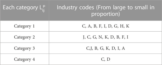
After obtaining the distance between stocks in the overall sample interval, we first select the 30 stocks with the closest distance in the neighborhood for each stock to construct new 31 × 31 distance matrices Di,total. The subscript i = 1, …, 100 represents one stock, and total represents the distance matrix we used for the full sample interval. Second, we consider 31 stocks as points to construct the point cloud data and conduct TDA on the complexes, mainly based on the persistence landscapes. Finally, we use the same method to calculate the Lp-norms of the persistence landscapes, called neighborhood norms. To explore the dynamic evolution of the stock market structure before and during the event, after determining the number of clusters using the elbow method, we performed a cluster analysis using the K-means on the neighborhood norms. The elbow plot of the neighborhood norms during the full-time interval is illustrated in Figure 7. When the number of clusters gradually increases from one to four, the SSE decreases in a decreasing trend with a larger magnitude, and when the number of clusters continues to increase from four to five or more, the decrease in SSE becomes small. Using the elbow method, we selected the elbow corner of SSE in figure K = 4 for the number of clusters. Therefore, we obtained the Lp-norms contained in each category, denoted
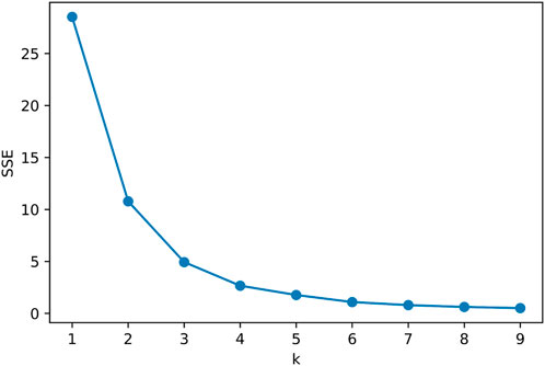
FIGURE 7. Elbow plot of the neighborhood norms for the overall sample interval. The lateral axis represents the number of clusters K, and the vertical axis represents the sum of squared errors (SSE) of the full sample. The bend in the line, the point where the SSE descent becomes slower, is evident.
The industry segmentation is determined by the main business of the listed company, which in turn influences the price through fundamental factors; therefore, so the volatility of stock prices in the same industry is more similar. Therefore, according to the latest SIC, we conduct in-depth research on 100 stocks by industry. Owing to the large number of industries involved, we represent them by industry codes1. We can draw the following conclusions from Table 3. In general, the distribution of stocks in most industries is more uniform and scattered, and the owning industries of several mass organizations, including stock structures, are rich. This is due to the influence of financial market psychology, such as the herd effect and market expectations, which are benign and reflect the normal characteristics of China’s stock markets. The first category is closely related to other stocks; it basically covers the representative stocks in each industry, such as wholesale and retail. Financial sector stocks are distributed in the second and third categories, which indicates that most are at the midstream level with surrounding connections because these play a role in stabilizing the stock markets. The manufacturing industry and so on dominate in all categories.
4.2 Stock correlation changes around critical dates and their mechanisms
Whether it is a complementary or a collaborative relationship, there are certain connections between industries. We want to provide a more accurate characterization of how the industry is changing and influenced by major events. Therefore, we use each of the aforementioned critical dates and the 50th day before them as the scope for the industry analysis. We then apply TDA to calculate the neighborhood norms separately for all stocks on a day t and use the K-means to cluster the norms, respectively. According to each elbow graph, K = 4 is always the optimal cluster number, and finally obtain the neighborhood norms
We present the changes in the neighborhood norms for the 100 stocks for each pair of dates in Figure 8. Although the L1-norms before and during events are different, they generally display a synchronous trend, that is, the neighborhood norms before events are always greater than those during events. This illustrates that when the event occurs, each stock is influenced by other stocks in all industries. It is more consistent with the norms of the overall sample interval, which indicates that there is risk linkage among stocks in various industries, and also demonstrates the stability and applicability of the norms and categorization.
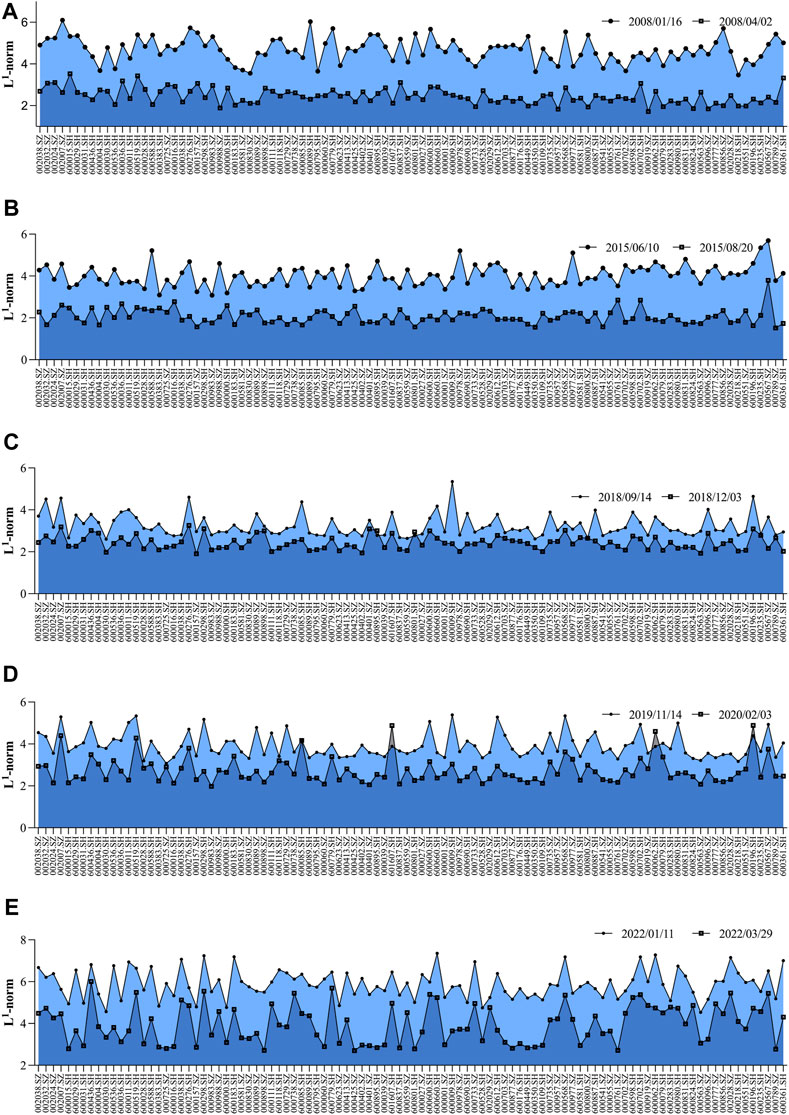
FIGURE 8. Comparison of neighborhood norms before and during events from (A–E), respectively. (A) Neighborhood norms of 100 stocks on 2008/01/16 and 2008/04/02. (B) Neighborhood norms of 100 stocks on 2015/06/10 and 2015/08/20. (C) Neighborhood norms of 100 stocks on 2018/09/14 and 2018/12/03. (D) Neighborhood norms of 100 stocks on 2019/11/14 and 2020/02/03. (E) Neighborhood norms of 100 stocks on 2022/01/11 and 2022/03/29.
We use K-means to cluster the neighborhood norms before and during events (Tables 4, 5, respectively). There are some industries where stocks are distributed and dispersed, both before and during events. For example, the manufacturing industry is in almost every category. This illustrates that China’s stocks in the manufacturing industry are in a relatively stable state before and during events. There are also some industries whose stocks have relatively significant changes in their distribution. For example, the mining and real estate industries have large changes in their categories in response to different shocks; that is, there is an increase in correlation of different magnitudes.
In 2008, the Subprime Lending Crisis caused significant changes in the stock markets. The stock correlation of building materials and furniture industries strengthened, indicating that the crisis had a very severe impact on export-dependent industries. There is also a significant increase in stock correlations in the mining industry. The crash in China’s stock markets in 2015 led to a significant increase in stock correlations in the farming, forestry, animal husbandry, and fishery industry and wholesale and retail trade, and so on. In 2018, industries were affected by the trade war between China and the U.S.; the changes in correlations are more consistent, and a few stocks have smaller changes. The COVID-19 pandemic in 2020 has dealt an irretrievable blow to the global real economy. Electrical, heat, gas, water production and supply industry, and so on. are mainly located in the first two categories, and wholesale and retail trade are mainly located in the first category; the correlation of all of them has increased significantly. In 2022, the COVID-19 outbreak was concentrated in Shanghai. The correlation between stocks in the electrician, heat, gas, and water production and supply industry and the real estate industry all increased significantly.
5 Conclusion
We use TDA and K-means to examine the variation in China’s stocks under major events. The main conclusions are as follows. First, according to the TDA and norms, when the financial crisis occurred, stocks were closely linked. During a major public event, the norms are obviously at a lower level, which reveals the strong correlations among the stocks. The norms can reasonably and effectively depict the volatility of the stock markets and accurately identify critical information. Second, the threshold network and its topological measures indicate that, with the arrival of the financial crisis, the correlation among sample stocks became increasingly close in the short term, but the heterogeneity of systemic risks caused by major events led to different changes in the degree of correlation between stock returns. Third, before an event, stocks in most industries were evenly distributed, and those in each community structure belonged to various industries. During an event, the stocks of each industry had a greater impact on the other stocks. Consistency and agglomeration reveal a risk linkage between the stocks of each industry. The impact of an event is systematic, with rapid risk and complex transmission paths. From another perspective, different industries were affected by different events with different direct and indirect impacts. When we examine some asset-specific issues or different countries’ stock markets, their persistence landscapes and norms change with the structure of stock prices, thus identifying the critical dates. Our methodology is generalizable and can be extended to other countries, where information about changes in other countries is closely linked to major events in their countries, and also to identify mutation dates and thus investigate market changes.
Based on our results, we propose the following suggestions. First, strengthen the target of financial coordination regulation. Furthermore, various industries should be divided into multiple levels of policy assistance and supervision according to the degree of correlation and the strength of impact to improve the efficiency of resource allocation in the vulnerable period of the financial markets. Second, the double effects of supply and demand have a profound effect on each industry, particularly when major events occur. The interdependence of each industry’s economy is evident, and a chain reaction is in effect. Therefore, we must provide risk protection for enterprises while simultaneously improving the efficiency of capital use and the fiscal deficit ratio to ensure sustainable financial development. We also believe that our methods have a guiding role in capturing market variability. In addition, as the world’s second-largest economy, frequent changes in China’s stock market are bound to affect other economic markets, even the global economy. We aim to conduct a deeper study on the stock markets, financial markets, and even the macroeconomy by adding more stock data, indicators, or statistical information and continue to expand the scope of research to explore the changes in global stock markets, financial markets, and even the macroeconomy. In future research, the use of Lp distance metrics matrix [27] can be attempted to classify and evaluate crises and risks based on TDA and machine learning to realize risk warning more effectively.
Data availability statement
The raw data supporting the conclusion of this article will be made available by the authors, without undue reservation.
Author contributions
HG: Conceptualization, Data curation, Formal Analysis, Methodology, Project administration, Software, Supervision, Validation, Visualization, Writing–original draft, Writing–review and editing. ZM: Data curation, Formal Analysis, Software, Visualization, Writing–original draft. BX: Data curation, Formal Analysis, Validation, Visualization, Writing–review and editing. All authors listed have made a substantial, direct, and intellectual contribution to the work and approved it for publication.
Funding
This research was funded by the National Natural Science Foundation of China-Shandong Joint Fund (No. U1806203), the National Social Science Foundation of China (No. 21BTJ072), the Shandong Key R & D (major scientific and technological innovation) Project (No. 2021CXGC010108), and the Shandong Undergraduate Teaching Reform Research Project (No. 2022096).
Conflict of interest
The authors declare that the research was conducted in the absence of any commercial or financial relationships that could be construed as a potential conflict of interest.
Publisher’s note
All claims expressed in this article are solely those of the authors and do not necessarily represent those of their affiliated organizations, or those of the publisher, the editors and the reviewers. Any product that may be evaluated in this article, or claim that may be made by its manufacturer, is not guaranteed or endorsed by the publisher.
Footnotes
1Farming, forestry, animal husbandry, and fishery industry-A, mining industry-B, manufacturing industry-C, electrical, heat, gas, and water production and supply-D, wholesale and retail trade-F, transportation, warehousing, and postal services-G, hotel and catering sectors-H, information transmission, software, and information technology services-I, finance-J, real estate-K, water conservancy, environment, and public facilities management industry-N.
References
1. James N, Menzies M. Association between covid-19 cases and international equity indices. Physica D Nonlinear Phenomena (2021) 417:132809. doi:10.1016/j.physd.2020.132809
2. Omay T, Iren P. Behavior of foreign investors in the malaysian stock market in times of crisis: a nonlinear approach. J Asian Econ (2019) 60:85–100. doi:10.1016/j.asieco.2018.11.002
3. Chen C, Tan D, Qin H, Wang B, Gao J. Analysis of systemic risk from the perspective of complex networks: overview and outlook. Control Theor Appl (2022) 39:2202–18. doi:10.7641/CTA.2021.10267
4. Diebold FX, Yılmaz K. On the network topology of variance decompositions: measuring the connectedness of financial firms. J Econom (2014) 182:119–34. doi:10.1016/j.jeconom.2014.04.012
5. Gong X, Xiong X, Zhang W. Research on systemic risk measurement and spillover effect of financial institutions in China. Manage World (2020) 36:65–82. doi:10.3969/j.issn.1002-5502.2020.08.007
7. Jia X, Su Y, Gao C. Var model in the application of the stock market risk analysis and empirical analysis. Chin J Manage Sci (2014) 22:336–41. doi:10.16381/j.cnki.issn1003-207x.2014.s1.061
8. Acharya VV, Pedersen LH, Philippon T, Richardson M. Measuring systemic risk. Rev Financial Stud (2016) 30:2–47. doi:10.1093/rfs/hhw088
9. Brownlees C, Engle RF. Srisk: a conditional capital shortfall measure of systemic risk. Rev Financial Stud (2016) 30:48–79. doi:10.1093/rfs/hhw060
10. Lin Y, Chen C, Liu Y. Identification of global systemic risk contagion path based on multiple motivations of international capital flow. Stat Res (2021) 38:42–60. doi:10.19343/j.cnki.11-1302/c.2021.12.004
11. Song Y, Lv J. The co-movement and risk spillover effects of Chinese and foreign stock markets under the impact of sudden events. J Quantitative Econ (2022) 13:15–33. doi:10.16699/b.cnki.jqe.2022.01.006
12. Liu X, Duan B, Xie F. A study of stock market risk spillover effects: an analysis based on evt-copula-covar model. The J World Economy (2011) 339:145–59. doi:10.19985/j.cnki.cassjwe.2011.11.009
13. Zhang L, Yang Z, Lu F. Empirical analysis of relevance of stock indicators based on complex network theory. Chin J Manage Sci (2014) 22:85–92. doi:10.16381/j.cnki.issn1003-207x.2014.12.012
14. An J, Wang W, Chen X. An empirical study of risk measurement in China’s stock market - taking the sse index as an example. Stat Manage (2015) 213:51–2. doi:10.3969/j.issn.1674-537X.2015.04.24
15. Robert G. Barcodes: the persistent topology of data. Bull Am Math Soc (2008) 45:61–75. doi:10.1090/S0273-0979-07-01191-3
16. Carlsson G. Topology and data. Bull Am Math Soc (2009) 46:255–308. doi:10.1090/s0273-0979-09-01249-x
17. Bubenik P. Statistical topology data analysis using persistence landscapes. J Machine Learn Res (2015) 16:77–102. doi:10.48550/arXiv.1207.6437
18. Bubenik P, Dlotko P. A persistence landscapes toolbox for topological statistics. J Symbolic Comput (2017) 78:91–114. doi:10.1016/j.jsc.2016.03.009
19. Gidea M, Katz Y. Topological data analysis of financial time series: landscapes of crashes. Physica A: Stat Mech its Appl (2018) 491:820–34. doi:10.1016/j.physa.2017.09.028
20. Guo H, Xia S, An Q, Zhang X, Sun W, Zhao X. Empirical study of financial crises based on topological data analysis. Physica A: Stat Mech its Appl (2020) 558:124956. doi:10.1016/j.physa.2020.124956
21. Goel A, Pasricha P, Mehra A. Topological data analysis in investment decisions. Expert Syst Appl (2020) 147:113222. doi:10.1016/j.eswa.2020.113222
22. Yen TW, Cheong SA. Using topological data analysis (tda) and persistent homology to analyze the stock markets in singapore and taiwan. Front Phys (2021) 9:572216. doi:10.3389/fphy.2021.572216
23. Munkres JR. Elements of algebraic topology. California: Addison Wesley (1984). doi:10.1201/9780429493911
24. Collins A, Zomorodian A, Carlsson G, Guibas LJ. A barcode shape descriptor for curve point cloud data. Comput Graphics (2004) 28:881–94. doi:10.1016/j.cag.2004.08.015
25. Cohen-Steiner D, Edelsbrunner H, Harer J. Stability of persistence diagrams. Discrete Comput Geometry (2007) 37:103–20. doi:10.1007/s00454-006-1276-5
26. Costa LDF, Rodrigues FA, Travieso G, Boas PRV. Characterization of complex networks: a survey of measurements. Adv Phys (2007) 56:167–242. doi:10.1080/00018730601170527
Keywords: topological data analysis, persistence landscape, Lp-norm, complex network, major public event, systemic financial risk
Citation: Guo H, Ming Z and Xing B (2023) Topological data analysis of Chinese stocks’ dynamic correlations under major public events. Front. Phys. 11:1253953. doi: 10.3389/fphy.2023.1253953
Received: 06 July 2023; Accepted: 07 August 2023;
Published: 22 August 2023.
Edited by:
Marcin Wątorek, Cracow University of Technology, PolandReviewed by:
Max Menzies, Tsinghua University, ChinaNick James, The University of Melbourne, Australia
Copyright © 2023 Guo, Ming and Xing. This is an open-access article distributed under the terms of the Creative Commons Attribution License (CC BY). The use, distribution or reproduction in other forums is permitted, provided the original author(s) and the copyright owner(s) are credited and that the original publication in this journal is cited, in accordance with accepted academic practice. No use, distribution or reproduction is permitted which does not comply with these terms.
*Correspondence: Hongfeng Guo, Z3VvaG9uZ2ZlbmdAc2R1ZmUuZWR1LmNu
 Hongfeng Guo
 Ziwei Ming
 Bing Xing
