Dynamics of a droplet in shear flow by smoothed particle hydrodynamics

1 Introduction

The deformation and breakup of droplets in shear flow are ubiquitous in engineering applications. On microfluidic chips, droplets are utilized for microbial cultivation and material transport [1,2], and a thorough understanding of their dynamics in confined flows may improve the efficiency of production and transportation. In other environmental and industrial applications such as protection against harmful aerosols, ink-jet printing and atomization in nozzles [3–7], liquid droplets are typically in gas flows. Accordingly, a decent knowledge on their dynamics with a high density/viscosity ratio against the matrix fluid is significant. To this end, a comprehensive investigation on the dynamics of a droplet in shear flow, which involves a wide range of Reynolds number, capillary number, confinements of the wall, viscosity/density ratio between the two phases, is called for.

Since pioneering works by Taylor on droplet deformation in shear and extensional flows [8,9], enormous theoretical and experimental studies have been conducted. A series of works by the group of Mason [10–12] further studied the deformation and burst of droplets, and even depicted the streamlines inside and around the droplets. Chaffey and Brenner [13] extended a previous analytical approximation to a second order form, which is crucial for the non-elliptic deformation of a highly viscous droplet under large shear rate. Barthes-Biesel and Acrivos [14] expressed the solution of creeping-flow equations in powers of deformation parameters and applied a linear stability theory to determine the critical values for the droplet breakup. Hinch and Acrivos [15] investigated theoretically the stability of a long slender droplet, which is largely deformed in shear flow. However, early analytical works rarely considered effects of finite Reynolds number or wall confinements. In addition, numerous experimental studies have been conducted on the droplet deformation and breakup [16–19], where not only the effects of viscosity ratio between the droplet and the matrix fluid [20,21], but also wall confinements [22,23] have been taken into account.

With advance in computational science, numerical simulation has become a popular approach to study droplet dynamics in the past decades. Boundary integral method was among the first to be applied to study deformation of droplets in stationary and transient states [24], non-Newtonian droplets [25], and migration of a droplet in shear flow [26]. Moreover, Li et al. [27] employed a volume-of-fluid (VOF) method and Galerkin projection technique to simulate the process of droplet breakup. In the work of Amani et al. [28], a conservative level-set (CLS) method built on a conservative finite-volume approximation is applied to study the effect of viscosity ratio and wall confinement on the critical capillary number. In addition, lattice Boltzmann method (LBM) has been widely employed to study deformation, breakup and coalescence of droplets [29–33]; to model viscoelastic droplet [34] and surfactant-laden droplet [35]. We note that an interface tracing technique such as VOF, CLS, a phase-field formulation, or immersed boundary method is often necessary by a flow solver based on Eulerian meshes.

As a Lagrangian method, smoothed particle hydrodynamics (SPH) method has some advantages in simulating multiphase flows. Since different phases are identified by different types of particles, the interface automatically emerges without an auxillary tracing technique, even for a very large deformation. Moreover, inertia and wall effects can be taken into account straightforward, in contrast to theoretical analysis or the boundary integral method. Since its inception in astrophysics, SPH method has been largely developed and widely applied in various flow problems [36,37]. Morris [38] considered the surface tension based on a continuous surface force model and simulated an oscillating two-dimensional rod in SPH. Hu et al. [39] proposed a multi-phase model that handles both macroscopic and mesoscopic flows in SPH, where a droplet in shear flow was selected as a benchmark to validate the method. Other improvements and modifications have also been proposed for SPH in the context of multiphase problems [40–43]. Furthermore, a droplet or matrix flow with special properties can also be considered. For example, Moinfar et al. [44] studied the drop deformation under simple shear flow of Giesekus fluids and Vahabi [45] investigated the effect of thixotropy on deformation of a droplet under shear flow. Saghatchi et al. [46] studied the dynamics of a 2D double emulsion in shear flow with electric field based on an incompressible SPH method. There are also studies on colliding and coalescence process of droplets by SPH [47,48]. Simulation of bubbles in liquid is similar, but can encounter special challenges [49], due to the reverse density/viscosity ratio as that of droplet in gas.

Previously, simulations of multiphase flows by SPH method often investigated specific circumstances. Therefore, the objective of this paper is two fold: firstly, to simulate an extensive range of parameters to examine the SPH method for multiphase flows; secondly, to fill gaps of unexplored range of parameters and systematically investigate their influence on the droplet dynamics. The rest of the paper is arranged as follows: in Section 2, we introduce the multiphase SPH method and a specific surface tension model. We present validations and extensive numerical results in Section 3. We summarize this work after discussions in Section 4.

2 Methods

2.1 Governing equations and surface tension model

We consider isothermal Navier-Stokes equations with a surface tension for multiphase flow in Lagrangian frame

$\begin{array}{cc}\hfill & \frac{d\rho }{dt}=-\rho \nabla \cdot \mathbf{v},\hfill \\ \hfill & \frac{d\mathbf{v}}{dt}=\frac{1}{\rho }\left(-\nabla p+{\mathbf{F}}_b+{\mathbf{F}}_v+{\mathbf{F}}_s\right),\hfill \end{array}(1)$

where ρ, v and p are density, velocity and pressure respectively. F_b is the body force, which is not considered in this study. F_v, F_s denote viscous force and surface tension at the interface between two phases, respectively.

Following previous studies of quasi-incompressible flow modeling [38], an artificial equation of state relating pressure to density can be written as

$p=c_s^2\left(\rho -{\rho }_{\text{ref}}\right),(2)$

where c_s is an artificial sound speed and ρ_ref is a reference density. Theoretically, subtracting the reference density has no influence on the gradient of pressure, but it can reduce the numerical error of SPH discretizations for the gradient operator.

For a Newtonian flow, the viscous force F_v simplifies to

${\mathbf{F}}_v=\mu {\nabla }^2\mathbf{v},(3)$

where μ is the dynamic viscosity. We assume surface tension to be uniform along the interface and do not consider Marangoni force. Therefore, the surface tension acts on the normal direction of the interface. Moreover, its magnitude depends on the local curvature as

${\mathbf{F}}_s=\sigma \kappa \widehat{\mathbf{n}}{\delta }_s,(4)$

where σ, κ, $\widehat{\mathbf{n}}$ are surface tension coefficient, curvature and unit normal vector to the concave side, respectively; δ_s is a surface delta function and its discrete form shall be described later.

To describe the surface tension at the interface between two fluids, a continuous surface tension model is adopted. As a matter of fact, surface tension my be written as the divergence of a tensor T [50,51]

$\sigma \kappa \widehat{\mathbf{n}}{\delta }_s=\nabla \cdot \mathbf{T},(5)$

where

$\mathbf{T}=\sigma \left(\mathbf{I}-\widehat{\mathbf{n}}\otimes \widehat{\mathbf{n}}\right){\delta }_s.(6)$

To represent a multiphase flow, we define a color function c and set a unique value for each phase, that is, c^I = 0 and c^II = 1 for the two phases, respectively. Apparently, the color function has a jump from 0 to 1 at the interface between phase I and II. Therefore, the unit normal vector can be represented by the normalized gradient of the color function as

$\widehat{\mathbf{n}}=\frac{\nabla c}{\left|\nabla c\right|},(7)$

and the surface delta function is replaced by the scaled gradient as

${\delta }_s=\left|\mathbf{n}\right|=\frac{\left|\nabla c\right|}{\left|c^{\text{I}}-c^{\text{II}}\right|}.(8)$

2.2 SPH method

In SPH, fluid is represented by moving particles carrying flow properties such as density, velocity and pressure. We largely follow the work of Hu and Adams [39] and provide a brief derivation here. Density of a particle is calculated by interpolating the mass of neighboring particles as

${\rho }_i=m_i{\displaystyle \sum _j}{W}_{ij},(9)$

where mass m_i is constant for every particle. W_ij denotes a weight function for interpolation

$W_{ij}=W\left({\mathbf{r}}_{ij},h\right),(10)$

where r_ij = r_i − r_j is a relative position vector from particle j to i and h is the smoothing length. We further define

$V_i=\frac{1}{{\sum }_j{W}_{ij}},(11)$

to be an equivalent volume of particle i so that V_i = m_i/ρ_i.

The pressure gradient can be computed as

$-{\left(\frac{1}{\rho }\nabla p\right)}_i=-{\displaystyle \sum _j}\left(V_i^2{p}_i+V_j^2{p}_j\right)\frac{\partial W}{\partial r_{ij}}{\mathbf{e}}_{ij},(12)$

where p_i and p_j are obtained by Eq. 2. The viscous force can be calculated as

${\left(\mu {\nabla }^2\mathbf{v}\right)}_i={\displaystyle \sum _j}\frac{2{\mu }_i{\mu }_j}{{\mu }_i+{\mu }_j}\left(V_i^2+V_j^2\right)\frac{{\mathbf{v}}_{ij}}{r_{ij}}\frac{\partial W}{\partial r_{ij}},(13)$

where v_ij = v_i − v_j is the relative velocity of particle i and j and $r_{ij}=\left|{\mathbf{r}}_{ij}\right|$ is the distance between them.

As suggested by Morris [38] and Hu et al. [39], a part of pressure contribution $\sigma \frac{d-1}{d}{\delta }_s$ is removed to avoid attractive force and improve the stability of the interactions between SPH particles. Therefore, we employ

${\mathbf{T}}^{\prime }=\sigma \left(\frac{1}{d}\mathbf{I}-\widehat{\mathbf{n}}\otimes \widehat{\mathbf{n}}\right){\delta }_s(14)$

to replace Eq. 6, where d is the spatial dimension. Combining Eqs 7, 8 and Eq. 14, we obtain

${\mathbf{T}}^{\prime }=\frac{\sigma }{\left|c^{\text{I}}-c^{\text{II}}\right|\left|\nabla c\right|}\left(\frac{{\left|\nabla c\right|}^2}{d}\mathbf{I}-\nabla c\otimes \nabla c\right).(15)$

The gradient of color function between phase I and phase II can be calculated in SPH as

$\nabla c_i=\frac{1}{V_i}{\displaystyle \sum _j}{V}_j^2\left(c_j-c_i\right)\frac{\partial W}{\partial r_{ij}}{\mathbf{e}}_{ij},(16)$

where c_i (or c_j) is initially assigned to be c^I or c^II according to which phase particle i (or j) consititutes. Substitute Eq. 16 into Eq. 15 to obtain stress tensor

${\mathbf{T}}_i^{\prime }=\frac{\sigma }{\left|\nabla c_i\right|\left|c^{\mathrm{I}}-c^{\mathrm{I}\mathrm{I}}\right|}\left(\frac{{\left|\nabla c_i\right|}^2}{d}\mathbf{I}-\nabla c_i\otimes \nabla c_i\right).(17)$

Finally, the surface force term is calculated by the stress tensor using the SPH expression for divergence

${\left(\sigma \kappa \widehat{\mathbf{n}}{\delta }_s\right)}_i={\displaystyle \sum _j}\frac{\partial W}{\partial r_{ij}}{\mathbf{e}}_{ij}\cdot \left(V_i^2{\mathbf{T}}_i^{\prime }+V_j^2{\mathbf{T}}_j^{\prime }\right).(18)$

It is simple to see that the discrete version of δ_s in SPH is

${\left({\delta }_s\right)}_i=\frac{1}{V_i\left|c^{\mathrm{I}}-c^{\mathrm{I}\mathrm{I}}\right|}\left|{\displaystyle \sum _j}{V}_j^2\left(c_j-c_i\right)\frac{\partial W}{\partial r_{ij}}{\mathbf{e}}_{ij}\right|,(19)$

which has a finite support to remove the singularity and distributes the surface tension onto a thin layer of two fluids across the interface.

2.3 Computational settings

The quintic kernel is adopted as weight function

$W=\varphi \left\{\begin{array}{cc}{\left(3-R\right)}^5-6{\left(2-R\right)}^5+15{\left(1-R\right)}^5\hfill & 0\le R<1;\hfill \\ {\left(3-R\right)}^5-6{\left(2-R\right)}^5\hfill & 1\le R<2;\hfill \\ {\left(3-R\right)}^5\hfill & 2\le R<3;\hfill \\ 0\hfill & R\ge 3,\hfill \end{array}\right.(20)$

where R = r/h and h is the smoothing length. ϕ is a normalization coefficient which equals 1/120, 7/(478π) and 1/(120π) in one, two and three dimensions, respectively. We set h = 1.2Δx with Δx as the initial spacing distance between particles. This means that the support domain of the kernel function is truncated at 3.6Δx, namely, the cutoff r_c = 3.6Δx. According to our tests, a smoothing length of 1.2Δx is almost optimal for an excellent accuracy while avoiding the pairing instability. A detailed discussion on this issue is referred to Price [52].

Since we adopt a weakly compressible formulation, the sound speed c_s should be large enough to restrict the density fluctuations. Based on a scale analysis, Morris et al. [38,53] suggested that $c_s^2$ should be comparable to the largest of

$\frac{U^2}{\mathrm{\Delta }},\frac{\mu U}{{\rho }_{0}L\mathrm{\Delta }},\frac{FL}{\mathrm{\Delta }},\frac{\sigma \kappa }{{\rho }_0\mathrm{\Delta }},(21)$

where Δ is the density variation and U, L, F, κ and σ are typical velocity, length, body force, curvature and surface tension coefficient, respectively. Accordingly, for multiphase flows the sound speed may be different for each phase. In all simulations, we set identical Δ ≤ 0.5% for each phase and calculate c_s accordingly.

At every time step, the minimal relative density is recorded among all particles, that is,

${\rho }_{\mathit{min}}=\mathit{min}\left\{\mathit{min}\left\{\frac{{\rho }_i}{{\rho }_0^{\mathrm{I}}}\right\},\mathit{min}\left\{\frac{{\rho }_j}{{\rho }_0^{\mathrm{I}\mathrm{I}}}\right\}\right\},(22)$

where particle i belongs to phase I and particle j belongs to phase II; ${\rho }_0^{\mathrm{I}}$, ${\rho }_0^{\mathrm{I}\mathrm{I}}$ are initial densities for the two phases, respectively. Thereafter, ${\rho }_{\text{ref}}^{\mathrm{I}}=0.99{\rho }_{\mathit{min}}{\rho }_0^{\mathrm{I}}$, ${\rho }_{\text{ref}}^{\mathrm{I}\mathrm{I}}=0.99{\rho }_{\mathit{min}}{\rho }_0^{\mathrm{I}\mathrm{I}}$ are subtracted as reference density for each phase in Eq. 2 to compute the particle pressure. This operation is performed to reduce numerical errors in calculating the pressure gradient while still keeping repulsive forces between particles.

The explicit velocity-Verlet method is adopted for time integration and a time step is chosen appropriately for stability [38].

3 Numerical results

We consider a shear flow generated by two parallel walls with opposite velocity of magnitude U. Periodic boundaries apply in the x direction. The computational domain is with length L and height H. A circular droplet with radius R₀ is initially located at the center of the computational domain, as shown in Figure 1A. The blue dashed lines represent periodic boundaries. The continuous phase has viscosity μ_c while the dispersed phase has viscosity μ_d = λμ_c.

FIGURE 1

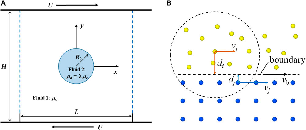
FIGURE 1. Schematic representation of a droplet in shear flow. (A) Initial geometry and parameters. (B) Treatment of no-slip boundary condition.

No-slip boundary condition is applied at the wall-fluid interfaces using the method proposed by Morris [53]. As shown in Figure 1B, yellow particles represent fluid and blue particles represent the boundary wall. The wall particles and boundary move with velocity v_b, which depends on the shear rate. But when a wall particle j is in the support domain of a fluid particle i, a given velocity v_j = d_j/d_i (v_b − v_i) + v_b is used to calculate the viscosity force between particle i and particle j in Eq. 13.

Five dimensionless parameters that determine the deformation of the droplet are Reynolds number $\mathit{Re}={\rho }_c\dot{\gamma }{R}_0^2/{\mu }_c$, Capillary number $Ca=\dot{\gamma }{R}_0{\mu }_c/\sigma$, confinement ratio R₀/H, viscosity ratio λ = μ_d/μ_c and density ratio α = ρ_d/ρ_c, where $\dot{\gamma }=2U/H$ is the shear rate, σ is the surface tension coefficient, ρ_d and μ_d are density and viscosity of the dispersed fluid phase inside the droplet while and ρ_c and μ_c are for the continuous fluid phase, respectively.

In Section 3.1, we study the deformation for an intact droplet while considering the effects due to the five dimensionless numbers. In Section 3.2, we examine the breakup of the droplet. In Section 3.3, we summarize the droplet dynamics for both intact shape and breakup in phase diagrams. In Section 3.4, we demonstrate the deformation and breakup with physical parameters of a water droplet in air flow as an industrial application.

3.1 Droplet deformation

When the shear is mild, the droplet remains intact and deforms to arrive at a stable shape eventually. The degree of droplet deformation can be quantified by the Taylor deformation parameter D = (A − B)/(A + B), where A is the greatest length and B is the breadth of the droplet as shown in Figure 2. To validate our method, we first compare our results of transient deformations with that of Sheth and Pozrikidis using immersed boundary method within the finite difference method [54]. We follow their work to set L = H = 4R₀ = 1, ρ_d = ρ_c = 1, μ_d = μ_c = 0.5 and adjust shear rate and surface tension. The two walls slide with velocities $\pm \frac{1}{2}\dot{\gamma }H$ to generate a clockwise rotation of the droplet. Two resolutions are considered for particles initially placed on squared lattice: Δx = 2R₀/25 and R₀/25, corresponding to the droplet containing N = 484 and 1976 particles, respectively.

FIGURE 2

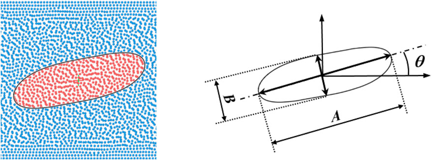
FIGURE 2. Trace of interface and parameters for the measurement of droplet deformation.

We present particle distributions and D as functions of time in Figure 3 for a typical simulation with Re = 0.125 and Ca = 0.45. We note that the deformation of the droplet may oscillate in time and its maximum elongation does not necessarily takes place at the steady state of a very long time.

FIGURE 3

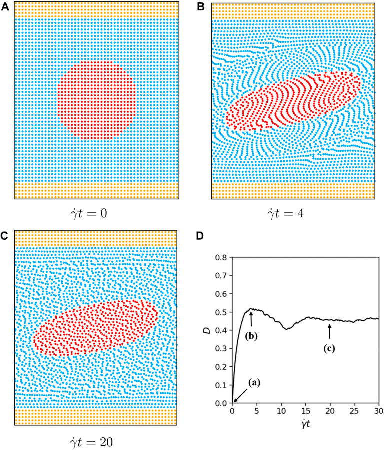
FIGURE 3. Particle distribution for H =4R₀, α = λ =1, Re =0.125, Ca =0.45, L =4R₀ at (A) initial configuration. (B) maximum elongation. (C) steady state. (D) Taylor deformation parameter as a function of time.

We further focus on the transient deformations in short time in Figure 4 so that we can compare our results with those of Sheth and Pozrikidis [54]. It can be readily seen that our results with low resolution Δx = 0.02 or N = 484 already reproduce the reference very well for different Reynolds numbers and/or capillary numbers. As the reference is within a rather short time period, some interesting phenomenon such as oscillation of the Taylor deformation parameter D is not captured, as indicated for Re = 12.5 and Ca = 0.025 on Figure 4D.

FIGURE 4

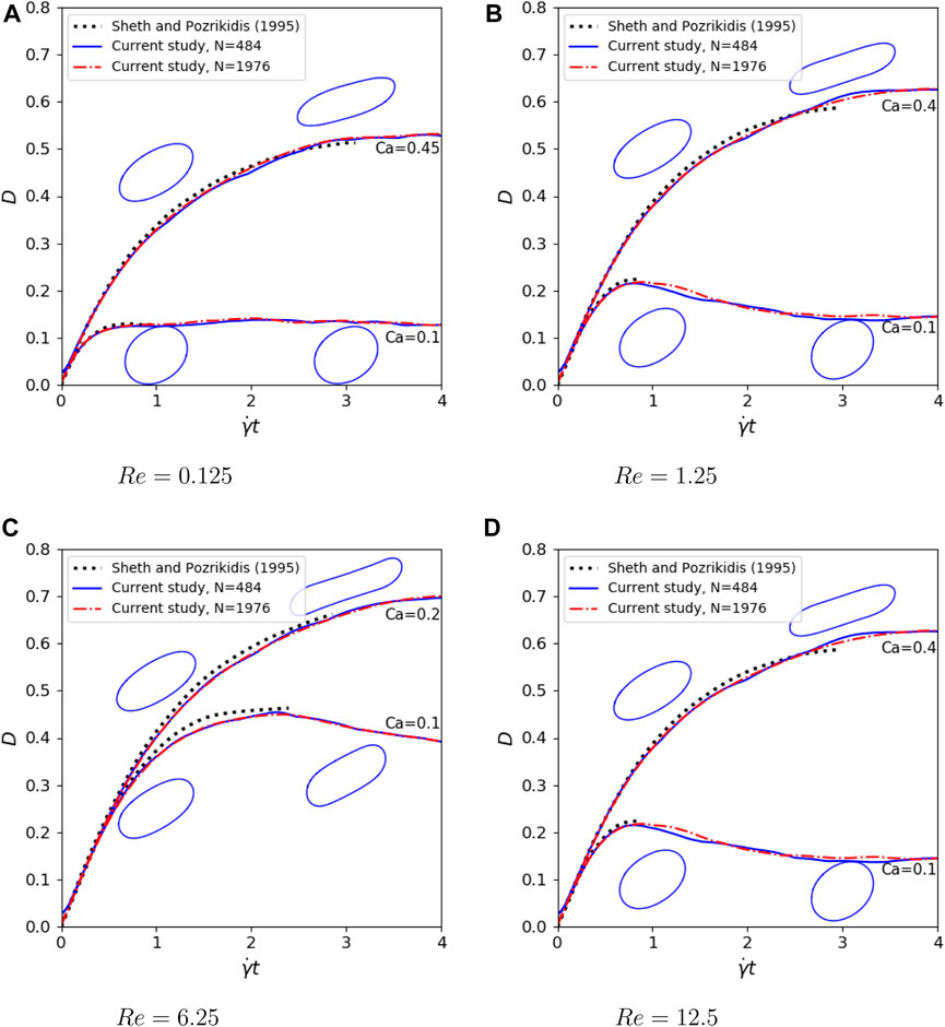
FIGURE 4. Transient deformations of a droplet compared with results of Sheth and Pozrikidis [54] with α = λ =1, H =4R₀, L =4R₀ and (A) Re =0.25, Ca =0.1,0.45. (B) Re =2.5, Ca =0.1,0.4. (C) Re =12.5, Ca =0.1,0.2. (D) Re =25, Ca =0.025,0.2.

To validate our method for vanishing Reynolds numbers, we calculate the stationary deformation and orientation of the droplet with respect to Ca. We follow Zhou and Pozrikidis [55] to set L = H = 8R₀ = 2, ρ_d = ρ_c = 1, μ_d = μ_c = 0.5 and adjust shear rate and surface tension accordingly. The deformation parameter D and orientation θ (defined on Figure 2) as functions of Ca (up to Ca = 1) for Re = 0.01 are shown in Figure 5. Results for Re = 0.1 and 1 are also given for comparison, where droplet breakup already takes places at Ca ≳ 0.4 for Re = 1. The difference between the results of Re = 0.1 and Re = 0.01 is insignificant and they both resemble the results of boundary integral method for Stokes flow [55]. We can readily conclude that Re = 0.1 is small enough to approximate the Stokes flow. We further present the contours and streamlines for a typical evolution of droplet deformation at vanishing Reynolds number in Figure 6.

FIGURE 5

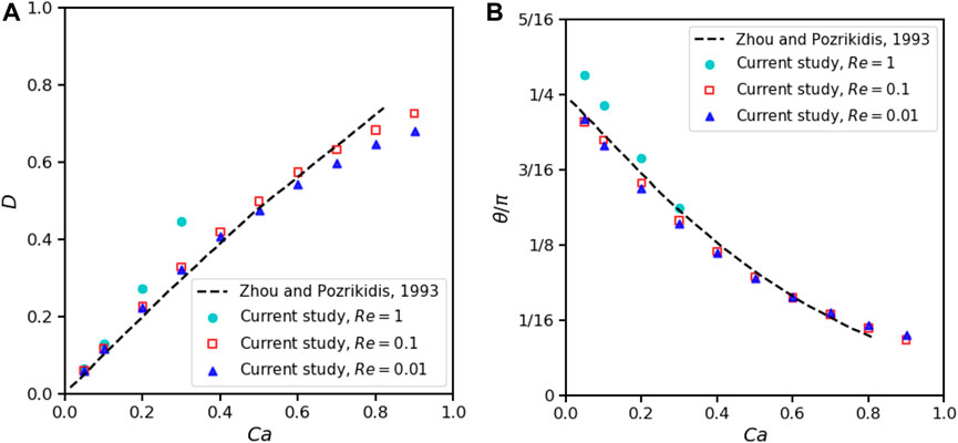
FIGURE 5. Effects of Re and Ca on 2D droplet deformation when α = λ =1, H =8R₀, L =8R₀. (A) Taylor deformation parameters. (B) Droplet orientation.

FIGURE 6

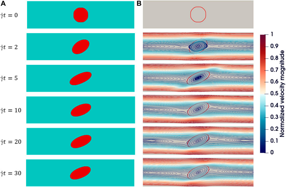
FIGURE 6. A typical evolution of deformation for an initially circular 2D droplet in shear flow: α = λ =1, Re =0.1, Ca =0.4, H =16R₀, L =16R₀. (A) Droplet deformation over time. (B) Streamlines: the color represents the magnitude of velocity and a red line indicates the droplet interface.

We commence to investigate the effects of confinement and set L = 16R₀ to minimize the periodic artifacts. We first restrict out attention to Re = 0.1, α = 1 and λ = 1. Four ratios of confinement are considered: H = 2.4R₀, 4R₀, 8R₀ and 16R₀. The deformation parameter as a function of Ca is shown in Figures 7A, B. As we can observe, a smaller distance of the two walls enhances the elongation of droplet and makes its long axis align more horizontally. As we relax the confinement, the relation between D and Ca becomes linear and the difference between H = 16R₀ and H = 8R₀ is already negligible. To further investigate the mechanism to the effects of wall confinement on the droplet deformation, we choose Ca = 0.4 plot the pressure around the droplet under four confinement ratio as shown in Figure 7C. We have subtracted a background pressure p₀ = 1000c², where 1,000 is the initial density and c = 0.707 is used under Ca = 0.4. For H = 2.4R₀ and H = 4R₀ we plotted the entire flow field region. For H = 8R₀ and H = 16R₀, we plot the middle region of 16R₀ × 4R0. We can clearly see the presence of low-pressure regions at both ends of the droplet. Under different wall confinements, the pressure in these low-pressure regions does not differ significantly. On the sides of the droplet in the middle, there are high-pressure regions, and the pressure in these high-pressure regions increases with an increase in the wall confinements. These high-pressure regions on the sides cause the droplet to elongate and become more horizontal. We can observe that there is only a slight difference in the pressure field between H = 8R₀ and H = 16R₀, so does the corresponding deformation of the droplet. A further exploration of why increasing the confinement causes an increase in pressure on sides of the droplet can be explained as follows: The proportion of the channel blocked by the droplet increases with the confinement. The outer flow is forced to bypass the droplet, resulting in a squeezing effect between the droplet and the wall. When the ratio R₀/H decreases, there is more space between the droplet and the wall to buffer this squeezing effect, dispersing the pressure over a larger area.

FIGURE 7

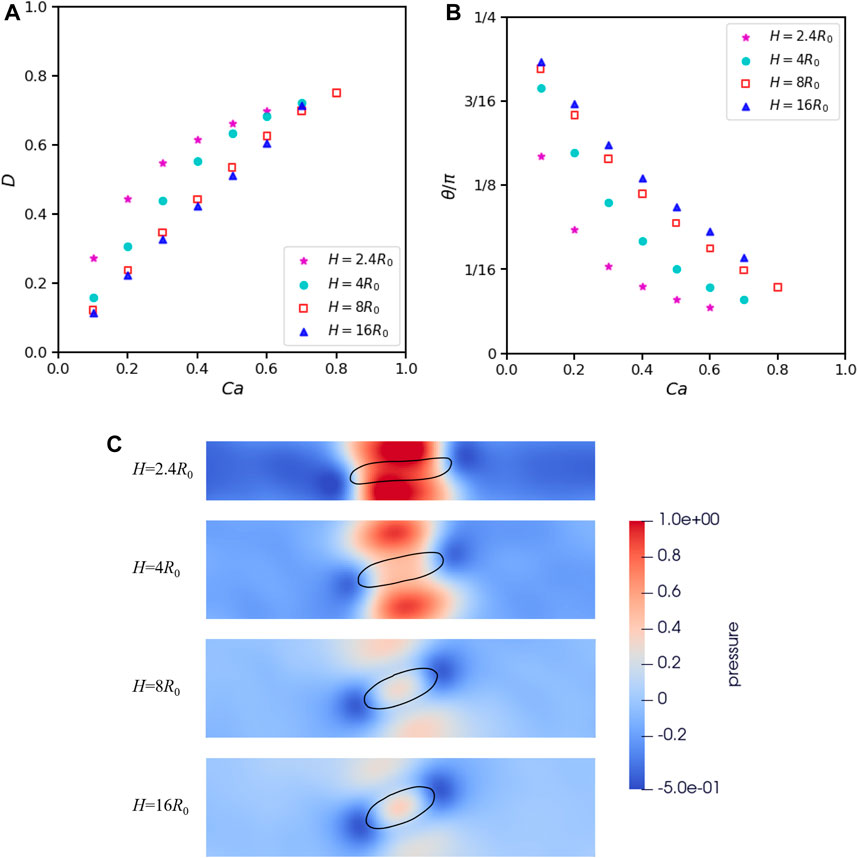
FIGURE 7. Effects of confinement ratio and Ca on 2D droplet deformation when α = λ =1, Re =0.1, L =16R₀. (A) Taylor deformation parameters. (B) Droplet orientation. (C) Pressure distribution around droplet under different confinements when Ca =0.4.

Furthermore, we simulate cases where the droplet and the matrix flow are two fluids with different physical properties. We first consider two fluids of the same density but with different viscosities. We choose a computational domain of 16R₀ × 16R₀ and set Re = 0.1, α = 1 and λ ranges from 0.1 to 10. Initial space Δx among nearest particles is 2R₀/25 so a droplet contains 484 particles. The deformation parameter as a function of Ca is shown in Figure 8. As we can observe, the deformation increases as λ increases from 0.1 to 10. In this range of λ, a droplet with lower viscosity has a smooth inside circulation and fast reaction which can reduce the elongation [16,20].

FIGURE 8

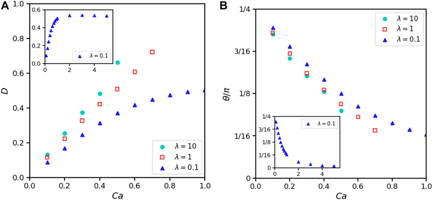
FIGURE 8. Effects of viscosity ratio λ and Ca on 2D droplet deformation when α =1, Re =0.1, H =16R₀, L =16R₀. (A) Taylor deformation parameters. (B) Droplet orientation.

The other case is that fluids inside and outside the droplet have the same viscosity but different densities. The sound speed is chosen according to the ratio of initial density to balance the pressure

$\frac{c_s^c}{c_s^d}=\frac{{\rho }_{\mathit{ref}}^d}{{\rho }_{\mathit{ref}}^c}=\frac{{\rho }_d}{{\rho }_c}=\alpha ,(23)$

where $c_s^c$, $c_s^d$ and ${\rho }_{\mathit{ref}}^c$, ${\rho }_{\mathit{ref}}^d$ are sound speeds and reference densities used for fluids outside and inside the droplet. As shown in Figure 9, the difference between deformations of droplet under density ratio 0.1–10 is very small except obvious lower inclination at small Ca when α = 0.1. In this small Reynolds number regime (Re = 0.1), the density ratio has negligible influence and only the capillary number determines the droplet deformation.

FIGURE 9

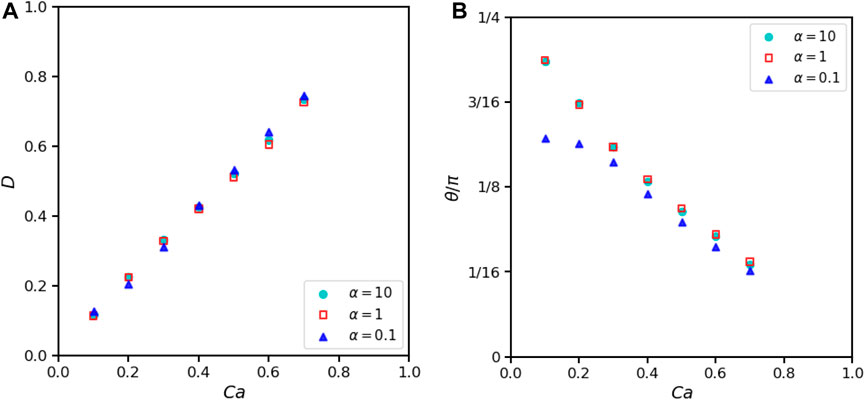
FIGURE 9. Effects of density ratio α and Ca on 2D droplet deformation when λ =1, Re =0.1, H =16R₀, L =16R₀. (A) Taylor deformation parameters. (B) Droplet orientation.

In 3D simulations, the width of simulation box W is an additional computational parameter compared to the 2D simulations. To compare with analytical predictions or experiment data, the length and width of simulation box are numerical and should be large enough. One set of parameters of Re = 0.1, Ca = 0.2, α = λ = 1, H = 4R₀ are selected and different length L and width W of simulation box are examined. According to our simulations, the deformation basically decreases with the increase of L and/or width W. We compare the Taylor deformation parameter D in steady states of our simulations with the analytical prediction of Shapira and Haber [56]. The differences between our results and analytical prediction under different L and W are plotted in Figure 10. It can be seen that when L is larger than 24R₀ and W is larger than 8R₀, the results has little change with the increase of L and/or W. Figure 11 shows the steady deformation of 3D droplets in shear flow when L = 24R₀, W = 8R₀, Re = 0.1 and α = λ = 1 with different Ca and confinement in H direction, compared with theoretical predictions of Shapira and Haber [56] and experiment data of Sibillo et al. [57]. Our results agree well with both anlaytical and experiment references at Ca = 0.1 and 0.2, whereas are closer to the experimental data at Ca = 0.3. The deformation increases with the confinement ratio R₀/H, which has the same trend as for 2D cases.

FIGURE 10

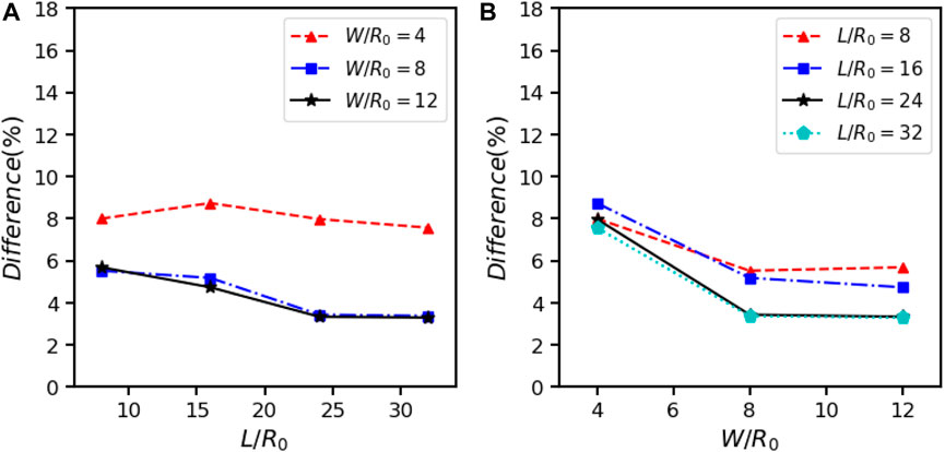
FIGURE 10. Effects of box length L and width W on the Taylor deformation parameter D of 3D droplet deformation when α = λ =1, Re =0.1, Ca =0.2, H =4R₀, compared to the analytical prediction of [56]. (A) Each line represents the same W/R₀. (B) Each line represents the same L/R₀.

FIGURE 11

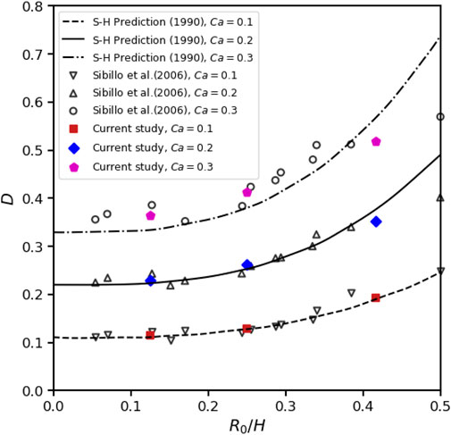
FIGURE 11. Effects of confinement ratio and Ca on 3D droplet deformation in shear flow when α =1 and Re =0.1, L =24R₀, W =8R₀, compared with predictions of Shapira and Haber [56] and experiment data of Sibillo et al. [57].

3.2 Droplet breakup

When the shear is strong, the droplet is over-stretched to break up. We find two patterns of breakup process under different viscosity ratios in simulations. As shown in Figure 12, when α = 1, λ = 0.2, Re = 0.1, Ca = 10, and L = H = 16R₀, a droplet is rotated and then stripped of its main body near the surface and gradually breaks apart. We call this breakup type A. This type is also found in the experiment study of Grace and they call it “tip streaming breakup” [20]. The conditions for type A breakup happening is exhibited in the next section. Figure 13 shows another set of typical snapshots of the droplet shape and flow fields in shear flow breaks when α = λ = 1, Re = 0.1, Ca = 0.9 and L = H = 16R₀. In this simulation, a droplet is stretched and its waist becomes slender and slender and finally breaks up. We call this breakup type B.

FIGURE 12

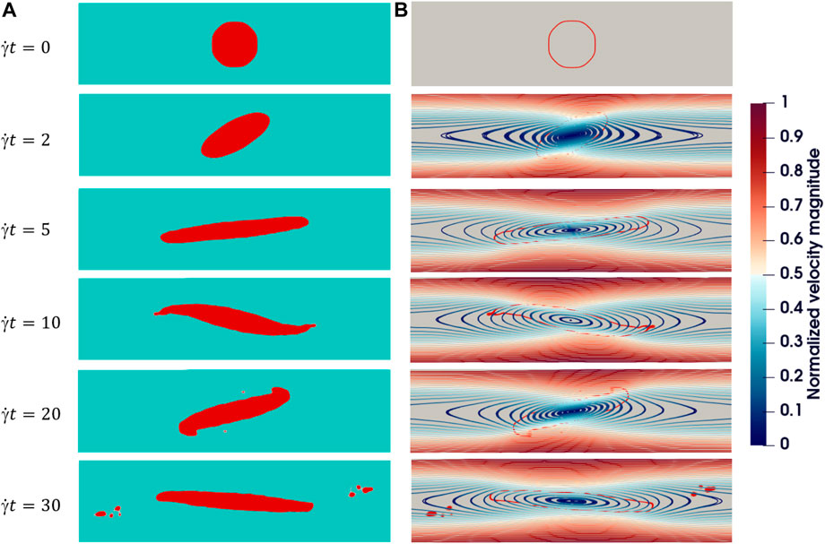
FIGURE 12. Breakup type (A) evolution of an initially circular 2D droplet breakup in shear flow with α =1, λ =0.2, Re =0.1, Ca =10, H =16R₀, L =16R₀. (A) Droplet shape. (B) Streamlines: The color represents the magnitude of velocity and red outlines in the background represent the droplet interface.

FIGURE 13

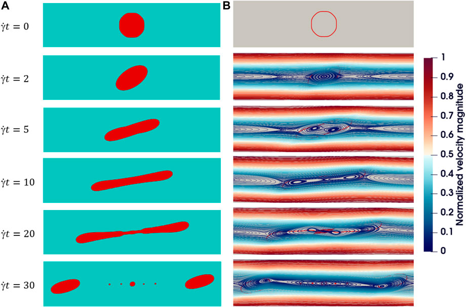
FIGURE 13. Breakup type (B) evolution of an initially circular 2D droplet breakup in shear flow with α = λ =1, Re =0.1, Ca =0.9, H =16R₀, L =16R₀. (A) Droplet shape. (B) Streamlines: The color represents the magnitude of velocity and red outlines in the background represent the droplet interface.

To encompass the breakup of a 3D droplet with a large elongation, we employ a rather long computational domain with L = 32R₀. Figure 14 shows the dynamics of the breakup with Re = 0.1, H = 2.857R₀, Ca = 0.46 and α = λ = 1. Left side are SPH particle distributions and right side are corresponding contour interfaces processed by SPH kernel interpolation into mesh cells. The color represents the magnitude of velocity. We adopt the same Ca and R₀/H as the experiment in creeping flow by Sibillo et al. [57]. The shape of the droplet in the breakup process of our simulation is very close to their experimental observation. Only a slight difference appears in the final stage: in the experiment, the droplet is divided into three main parts, while in our simulation the middle part continues to split into two smaller droplets. In contrast to the 2D case, a 3D droplet has a more slender shape before breaking up.

FIGURE 14

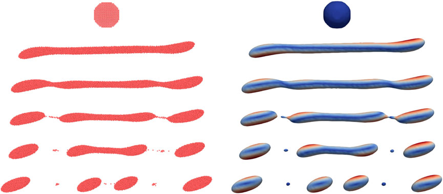
FIGURE 14. Evolution of an initially spherical 3D droplet breakup in shear flow when α = λ =1, Re =0.1, Ca =0.46, H =2.857R₀, L =16R₀: particle distribution (left) and interface (right).

3.3 Phase diagram

To clearly visualize the states of a droplet in different conditions, we consider a range of Reynolds numbers, capillary numbers, and confinements/density/viscosity ratios and summarize our simulation results into phase diagrams. Thereafter, we may estimate the critical capillary number Ca_c that segments the intact and breakup states and further investigate how it is influenced by other dimensionless parameters.

For λ = α = 1, we perform a group of 2D simulations with different Reynolds number Re = 0.01, 0.1, 1, 10 and confinement H = 2.4R₀, 4R₀, 8R₀, 16R₀ with Ca ∈ [0.1, 1.1] and L = 16R₀. For a general overview, the states of the droplet are summarized in Figure 15. To get a clear view, we slice the phase diagram by two perspectives. Firstly, we divide results into groups of the same confinement to reveal the influence of Re on Ca_c as shown in Figure 16. Overall it is apparent that a higher Re reduces Ca_c. Three scenarios are special: under confinement H = 2.4R₀, 4R₀ and 8R₀, we can not differentiate Ca_c between Re = 0.01 and 0.1.

FIGURE 15

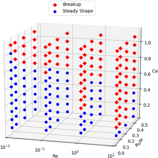
FIGURE 15. Phase diagram of 2D droplets states under different confinement, Re and Ca when α = λ =1, L =16R₀.

FIGURE 16

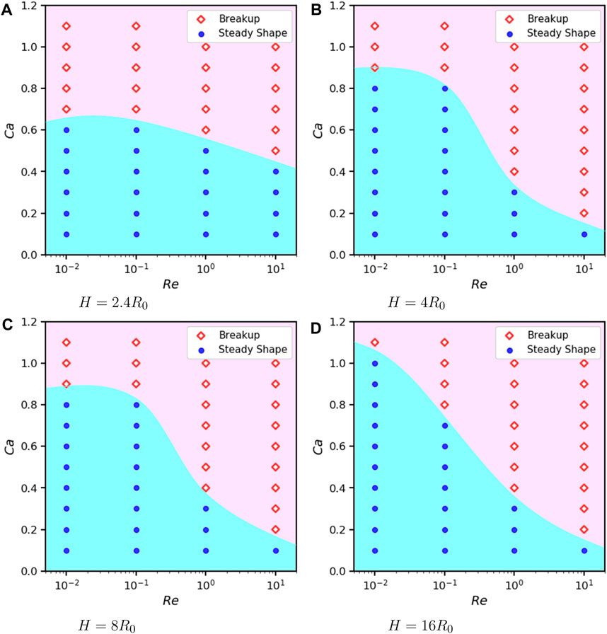
FIGURE 16. Phase diagram of 2D droplets states under different confinement, Re and Ca when α = λ =1, L =16R₀ and (A) H =2.4R₀. (B) H =4R₀. (C) H =8R₀. (D) H =16R₀.

From another perspective of Ca versus confinement ratio for each Re on Figure 17, we are not able to find a universal pattern. Under Re = 0.01, Ca_c decreases with R₀/H while under Re = 10, Ca_c increases with R₀/H. Whereas, under Re = 0.1 and 1, Ca_c has no monotonic relation with R₀/H.

FIGURE 17

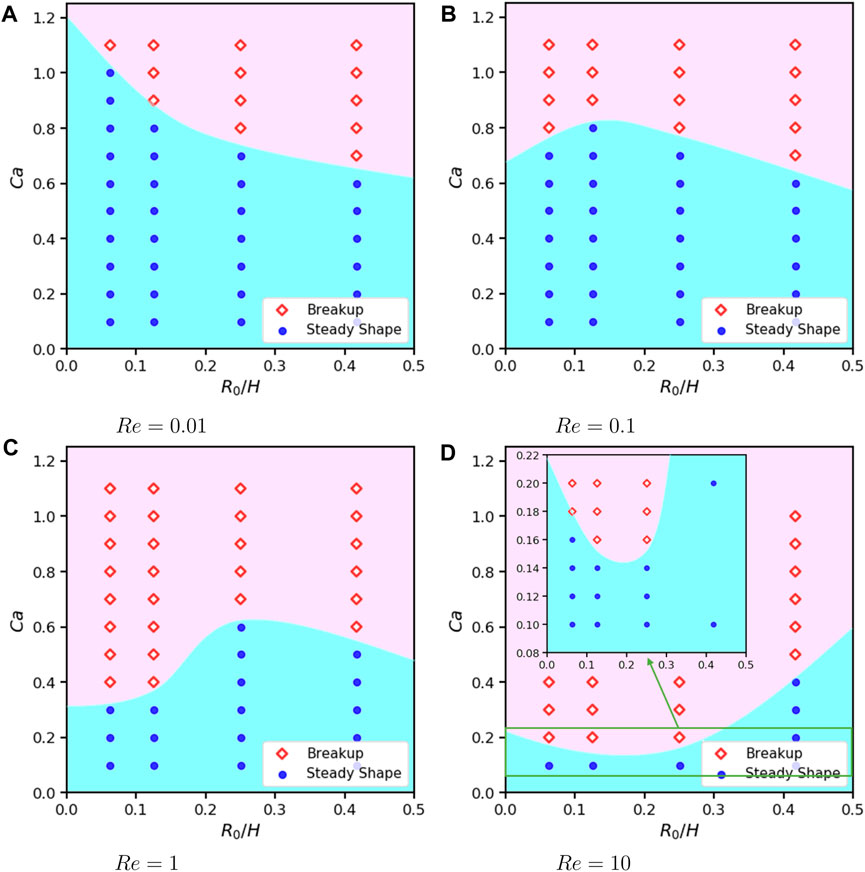
FIGURE 17. Phase diagram of 2D droplets states under different confinement, Re and Ca when α = λ =1, L =16R₀ and (A) Re =0.01. (B) Re =0.1. (C) Re =1. (D) Re =10.

Furthermore, we investigate effects of viscosity ratio λ = μ_d/μ_c ∈ [0.1, 10] on the droplet dynamics for Re = 0.1 and three confinement ratios H = 4R₀, 8R₀ and 16R₀. The results are shown in Figure 18. For breakup type A, the droplet rotates and is stripped off as described in Section 3.2; Breakup type B represents that a droplet is stretched and breaks up in the middle. Under Re = 0.1, type A is observed only if the droplet has a much smaller viscosity compare to the matrix fluid. Overall, Ca_c decreases with the increase of λ. However, we notice a flatten trend or even a reverse trend with small difference for Ca_c from λ = 5 to λ = 10, as shown on the insets of Figure 18. According to the study of Karam et al. and Grace [16,20], a maximum transfer of energy takes place across an interface, which demands this trend.

FIGURE 18

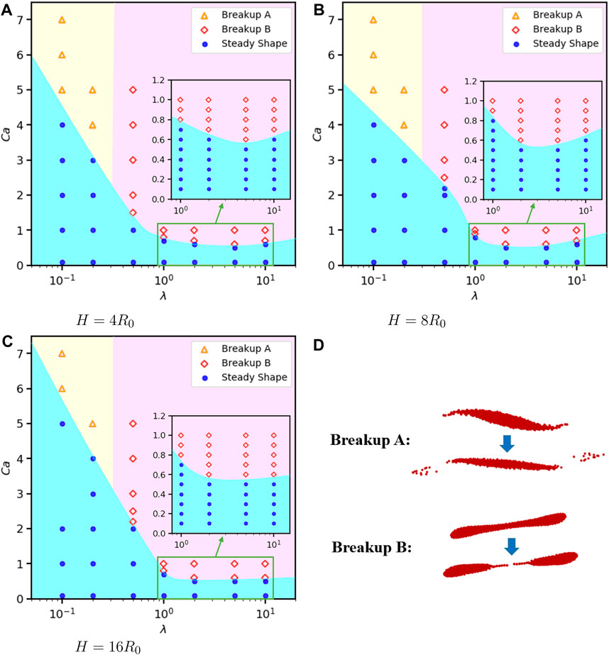
FIGURE 18. Phase diagram of 2D droplets states under different confinement, viscosity ratios λ and Ca when α =1, Re =0.1, L =16R₀. (A) H =4R₀. (B) H =8R₀. (C) H =16R₀. (D) two patterns of breakup.

Due to highly computational cost in 3D, we only consider a moderate confinement H/R₀ = 4 and perform a group of simulations to draw a phase diagram in the plane of Ca and Re, as shown in Figure 19. The size of the simulation box is L = 32R₀, W = 8R₀, H = 4R₀. As in 2D case, the critical Ca_c decreases with increasing Re in 3D, as shown in in Figure 16. However, the critical capillary number Ca_c in 3D case is significantly smaller than that of 2D case.

FIGURE 19

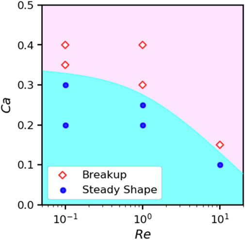
FIGURE 19. Phase diagram of 3D droplets states under different Re and Ca when α = λ =1, H =4R₀, L =32R₀, W =8R₀.

3.4 Water droplet in air flow

As one specific application, we employ our method to predict the breakup of a water droplet in shear flow of air. The critical capillary number or the shear rate determined is helpful to design an effective atomization device. Actual physical properties of water and air around 20°C are adopted: ρ_d = 998.2 kg ⋅ m⁻³, μ_d = 1.0087 × 10⁻³ Pa ⋅ s and ρ_c = 1.205 kg ⋅ m⁻³, μ_c = 1.81 × 10⁻⁵ Pa ⋅ s are set for water (dispersed) phase and air (continuous) phase, respectively; surface tension coefficient σ = 72.75 × 10⁻³ N ⋅ m⁻¹ is set for the water-air interface.

We perform a relative large range of Reynolds numbers and depict a phase diagram on the plane of Re and Ca in logarithmic-logarithmic scales on Figure 20. This allows us to connect the results with the same droplet size and observe its behavior while changing Re and Ca. Points on each dotted line represent the droplet of the same radius, as marked in the figure. For example, we have a line of dynamics for the droplet with R₀ = 10μm under shear rates of 1 × 10⁶s⁻¹, 2 × 10⁶s⁻¹, 5 × 10⁶s⁻¹, 1 × 10⁷s⁻¹, 2 × 10⁷s⁻¹; another line of dynamics for the droplet with R₀ = 100μm under shear rates of 5 × 10⁴s⁻¹, 1 × 10⁵s⁻¹, 2 × 10⁵s⁻¹, 5 × 10⁵s⁻¹, 1 × 10⁶s⁻¹. Furthermore, we observe that if the Re is on the order of 100, the critical Ca for breakup is very sensitive to Re. We also perform a group of 3D simulations for a droplet with R₀ = 50μm under shear rates of 1 × 10⁵s⁻¹, 2 × 10⁵s⁻¹, 5 × 10⁵s⁻¹, 1 × 10⁶s⁻¹, 2 × 10⁶s⁻¹. The 3D results for the critical point of breakup is close to that of the 2D results.

FIGURE 20

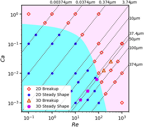
FIGURE 20. Diagram for states of water droplets in air shear flow under different Re and Ca when H =16R₀, L =16R₀.

4 Conclusion and disucssion

In this study, we employed a multi-phase SPH method to simulate droplet deformation and breakup subjected to a simple shear flow in an extensive range of physical parameters. We performed both 2D and 3D simulations and validated them by benchmarks: transient deformations and steady shapes of droplets are compared with previous simulations, analytical derivations and experimental data. These results indicate that the method is reliable to simulate droplet dynamics in general. We wish to emphasize the convenience of SPH method in simulating multi-phase problems, as we can leverage on its Lagrangian nature and differentiate different phases by particle species. In addition, the algorithm and data structure for 2D and 3D simulations have tiny difference and therefore, it is a simple task to extend the code from 2D to 3D. Economical 2D simulations allow us to investigate a wide range of physical parameters in five dimensions, which serve as a guide to 3D realistic situations. From the results, we come to the following conclusions.

(1) A larger Reynolds number Re or capillary number Ca leads to a more considerable deformation of the droplet. The transient and steady-state deformations of the droplet in our study are in good agreement with the previous studies but beyond their time limits [54,55].

(2) Under low Reynolds number (Re = 0.1), a stronger confinement due to the walls enhances the steady-state deformation in both 2D and 3D simulations. When the walls are separated further apart, the Taylor deformation parameter is almost linear with respect to Ca. The influence of confinement on the deformation of a droplet has been studied by Shapira and Haber by a first-order analytical solution based on Lorentz’s reflection method. They proved that the walls do not influence the shape of deformed droplet but increases the deformation magnitude with a term of order ${\left(R_0/H\right)}^3$ [56]. The experiment data of Sibillo et al. illustrate satisfactory agreement with the predictions of Shapira and Haber except for the droplet being within a small gap, where the reflection analysis is expected to fail [57]. Our 3D simulation results resemble the whole set of experiment data even when the droplet is within the small gap, which suggests the method as an applicative tool for more realistic situations in microfluidics.

(3) The effects of wall confinement on the critical capillary number Ca_c are not universal under different Re. When Re = 0.1, a closer gap of walls reduces Ca_c. This is because a closer gap of walls increases the deformation as described above. But when Re is larger, the relation between Ca_c and the confinement ratio is unclear. From our observation, this non-monotonic relation results from an interplay of influences by the shear strength and the stability of the whole flow field. On the one hand, the shear stress transferred to the droplet from the wall is more pronounced in stronger confinement [56], thus closer walls reduce the Ca_c. On the other hand, the narrower channel reduces the instability of the flow and restricts droplet movements, thus increases the Ca_c.

(4) Under Re = 0.1 and the range of viscosity ratio $\lambda \in \left[0.1,1\right]$, a higher λ causes a larger deformation. The effect of λ on Ca_c is not monotonic when λ > 1 and there is a minimum value of Ca_c between λ = 1 and λ = 10. The existence of a minimal Ca_c among different λ has also been found by previous experiment studies [16,20], when λ is about 1. The discrepancy between our results and the previous ones are attributed to the difference between 2D and 3D cases. At the same Re, the influence of density ratio on droplet deformation is much smaller compared with that of the viscosity ratio.

(5) As an application, a phase diagram obtained by actual physical parameters of water and air is depicted to predict the magnitude of shear rate for breaking a droplet of certain size, which is helpful in the designing atomization nozzles.

Data availability statement

The original contributions presented in the study are included in the article, further inquiries can be directed to the corresponding author.

Author contributions

KW: Formal Analysis, Investigation, Methodology, Validation, Writing–original draft, Writing–review and editing. HL: Formal Analysis, Supervision, Validation, Writing–review and editing. CZ: Conceptualization, Funding acquisition, Writing–review and editing. XB: Conceptualization, Formal Analysis, Funding acquisition, Supervision, Writing–review and editing.

Funding

The authors declare financial support was received for the research, authorship, and/or publication of this article. The authors declare that this study received funding from the national natural science foundation of China under grant number: 12172330. This study also received funding from Hangzhou Shiguangji Intelligent Electronics Technology Co., Ltd, Hangzhou, China. The funder was not involved in the study design, collection, analysis, interpretation of data, the writing of this article, or the decision to submit it for publication.

Conflict of interest

Author CZ was employed by Hangzhou Shiguangji Intelligient Electronics Technology Co., Ltd.

The remaining authors declare that the research was conducted in the absence of any commercial or financial relationships that could be construed as a potential conflict of interest.

Publisher’s note

All claims expressed in this article are solely those of the authors and do not necessarily represent those of their affiliated organizations, or those of the publisher, the editors and the reviewers. Any product that may be evaluated in this article, or claim that may be made by its manufacturer, is not guaranteed or endorsed by the publisher.

References

1. Anna SL. Droplets and bubbles in microfluidic devices. Annu Rev Fluid Mech (2016) 48:285–309. doi:10.1146/annurev-fluid-122414-034425

CrossRef Full Text | Google Scholar

2. Dressler OJ, Casadevall i Solvas X, DeMello AJ. Chemical and biological dynamics using droplet-based microfluidics. Annu Rev Anal Chem (2017) 10:1–24. doi:10.1146/annurev-anchem-061516-045219

CrossRef Full Text | Google Scholar

3. Liu J, Hao M, Chen S, Yang Y, Li J, Mei Q, et al. Numerical evaluation of face masks for prevention of covid-19 airborne transmission. Environ Sci Pollut Res (2022) 29:44939–53. doi:10.1007/s11356-022-18587-3

CrossRef Full Text | Google Scholar

4. Lohse D. Fundamental fluid dynamics challenges in inkjet printing. Annu Rev Fluid Mech (2022) 54:349–82. doi:10.1146/annurev-fluid-022321-114001

CrossRef Full Text | Google Scholar

5. Aydin O, Unal R. Experimental and numerical modeling of the gas atomization nozzle for gas flow behavior. Comput Fluids (2011) 42:37–43. doi:10.1016/j.compfluid.2010.10.013

CrossRef Full Text | Google Scholar

6. Si C, Zhang X, Wang J, Li Y. Design and evaluation of a laval-type supersonic atomizer for low-pressure gas atomization of molten metals. Int J Minerals, Metall Mater (2014) 21:627–35. doi:10.1007/s12613-014-0951-4

CrossRef Full Text | Google Scholar

7. Xu Z, Wang T, Che Z. Droplet deformation and breakup in shear flow of air. Phys Fluids (2020) 32:052109. doi:10.1063/5.0006236

CrossRef Full Text | Google Scholar

8. Taylor GI. The viscosity of a fluid containing small drops of another fluid. Proc R Soc Lond Ser A, Containing Pap a Math Phys Character (1932) 138:41–8.

Google Scholar

9. Taylor GI. The formation of emulsions in definable fields of flow. Proc R Soc Lond Ser A, containing Pap a Math Phys character (1934) 146:501–23.

Google Scholar

10. Bartok W, Mason S. Particle motions in sheared suspensions: viii. singlets and doublets of fluid spheres. J Colloid Sci (1959) 14:13–26. doi:10.1016/0095-8522(59)90065-0

CrossRef Full Text | Google Scholar

11. Rumscheidt F-D, Mason S. Particle motions in sheared suspensions xii. deformation and burst of fluid drops in shear and hyperbolic flow. J Colloid Sci (1961) 16:238–61. doi:10.1016/0095-8522(61)90003-4

CrossRef Full Text | Google Scholar

12. Torza S, Henry C, Cox R, Mason S. Particle motions in sheared suspensions. xxvi. streamlines in and around liquid drops. J Colloid Interf Sci (1971) 35:529–43. doi:10.1016/0021-9797(71)90211-6

CrossRef Full Text | Google Scholar

13. Chaffey CE, Brenner H. A second-order theory for shear deformation of drops. J Colloid Interf Sci (1967) 24:258–69. doi:10.1016/0021-9797(67)90229-9

CrossRef Full Text | Google Scholar

14. Barthes-Biesel D, Acrivos A. Deformation and burst of a liquid droplet freely suspended in a linear shear field. J Fluid Mech (1973) 61:1–22. doi:10.1017/s0022112073000534

CrossRef Full Text | Google Scholar

15. Hinch E, Acrivos A. Long slender drops in a simple shear flow. J Fluid Mech (1980) 98:305–28. doi:10.1017/s0022112080000171

CrossRef Full Text | Google Scholar

16. Karam H, Bellinger J. Deformation and breakup of liquid droplets in a simple shear field. Ind Eng Chem Fundamentals (1968) 7:576–81. doi:10.1021/i160028a009

CrossRef Full Text | Google Scholar

17. Flumerfelt RW. Drop breakup in simple shear fields of viscoleastic fluids. Ind Eng Chem Fundamentals (1972) 11:312–8. doi:10.1021/i160043a005

CrossRef Full Text | Google Scholar

18. Stone HA, Bentley B, Leal L. An experimental study of transient effects in the breakup of viscous drops. J Fluid Mech (1986) 173:131–58. doi:10.1017/s0022112086001118

CrossRef Full Text | Google Scholar

19. Guido S, Villone M. Three-dimensional shape of a drop under simple shear flow. J rheology (1998) 42:395–415. doi:10.1122/1.550942

CrossRef Full Text | Google Scholar

20. Grace HP. Dispersion phenomena in high viscosity immiscible fluid systems and application of static mixers as dispersion devices in such systems. Chem Eng Commun (1982) 14:225–77. doi:10.1080/00986448208911047

CrossRef Full Text | Google Scholar

21. Stone HA, Leal LG. The influence of initial deformation on drop breakup in subcritical time-dependent flows at low Reynolds numbers. J Fluid Mech (1989) 206:223–63. doi:10.1017/s0022112089002296

CrossRef Full Text | Google Scholar

22. Vananroye A, Van Puyvelde P, Moldenaers P. Effect of confinement on droplet breakup in sheared emulsions. Langmuir (2006) 22:3972–4. doi:10.1021/la060442+

PubMed Abstract | CrossRef Full Text | Google Scholar

23. Vananroye A, Van Puyvelde P, Moldenaers P. Effect of confinement on the steady-state behavior of single droplets during shear flow. J rheology (2007) 51:139–53. doi:10.1122/1.2399089

CrossRef Full Text | Google Scholar

24. Kennedy MR, Pozrikidis C, Skalak R. Motion and deformation of liquid drops, and the rheology of dilute emulsions in simple shear flow. Comput Fluids (1994) 23:251–78. doi:10.1016/0045-7930(94)90040-x

CrossRef Full Text | Google Scholar

25. Toose E, Geurts B, Kuerten J. A boundary integral method for two-dimensional (non)-Newtonian drops in slow viscous flow. J non-newtonian Fluid Mech (1995) 60:129–54. doi:10.1016/0377-0257(95)01386-3

CrossRef Full Text | Google Scholar

26. Uijttewaal W, Nijhof E. The motion of a droplet subjected to linear shear flow including the presence of a plane wall. J Fluid Mech (1995) 302:45–63. doi:10.1017/s0022112095004009

CrossRef Full Text | Google Scholar

27. Li J, Renardy YY, Renardy M. Numerical simulation of breakup of a viscous drop in simple shear flow through a volume-of-fluid method. Phys Fluids (2000) 12:269–82. doi:10.1063/1.870305

CrossRef Full Text | Google Scholar

28. Amani A, Balcázar N, Castro J, Oliva A. Numerical study of droplet deformation in shear flow using a conservative level-set method. Chem Eng Sci (2019) 207:153–71. doi:10.1016/j.ces.2019.06.014

CrossRef Full Text | Google Scholar

29. Xi H, Duncan C. Lattice Boltzmann simulations of three-dimensional single droplet deformation and breakup under simple shear flow. Phys Rev E (1999) 59:3022–6. doi:10.1103/physreve.59.3022

CrossRef Full Text | Google Scholar

30. van der Sman RG, Van der Graaf S. Emulsion droplet deformation and breakup with lattice Boltzmann model. Comp Phys Commun (2008) 178:492–504. doi:10.1016/j.cpc.2007.11.009

CrossRef Full Text | Google Scholar

31. Farokhirad S, Lee T, Morris JF. Effects of inertia and viscosity on single droplet deformation in confined shear flow. Commun Comput Phys (2013) 13:706–24. doi:10.4208/cicp.431011.260112s

CrossRef Full Text | Google Scholar

32. Komrakova A, Shardt O, Eskin D, Derksen J. Lattice Boltzmann simulations of drop deformation and breakup in shear flow. Int J Multiphase Flow (2014) 59:24–43. doi:10.1016/j.ijmultiphaseflow.2013.10.009

CrossRef Full Text | Google Scholar

33. Huang B, Liang H, Xu J. Lattice Boltzmann simulation of binary three-dimensional droplet coalescence in a confined shear flow. Phys Fluids (2022) 34:032101. doi:10.1063/5.0082263

CrossRef Full Text | Google Scholar

34. Wang D, Tan DS, Khoo BC, Ouyang Z, Phan-Thien N. A lattice Boltzmann modeling of viscoelastic drops’ deformation and breakup in simple shear flows. Phys Fluids (2020) 32:123101. doi:10.1063/5.0031352

CrossRef Full Text | Google Scholar

35. Zong Y, Zhang C, Liang H, Wang L, Xu J. Modeling surfactant-laden droplet dynamics by lattice Boltzmann method. Phys Fluids (2020) 32:122105. doi:10.1063/5.0028554

CrossRef Full Text | Google Scholar

36. Monaghan J. Smoothed particle hydrodynamics and its diverse applications. Annu Rev Fluid Mech (2012) 44:323–46. doi:10.1146/annurev-fluid-120710-101220

CrossRef Full Text | Google Scholar

37. Ye T, Pan D, Huang C, Liu M. Smoothed particle hydrodynamics (sph) for complex fluid flows: recent developments in methodology and applications. Phys Fluids (2019) 31:011301. doi:10.1063/1.5068697

CrossRef Full Text | Google Scholar

38. Morris JP. Simulating surface tension with smoothed particle hydrodynamics. Int J Numer Methods Fluids (2000) 33:333–53. doi:10.1002/1097-0363(20000615)33:3<333::aid-fld11>3.0.co;2-7

CrossRef Full Text | Google Scholar

39. Hu XY, Adams NA. A multi-phase sph method for macroscopic and mesoscopic flows. J Comput Phys (2006) 213:844–61. doi:10.1016/j.jcp.2005.09.001

CrossRef Full Text | Google Scholar

40. Wang Z-B, Chen R, Wang H, Liao Q, Zhu X, Li S-Z. An overview of smoothed particle hydrodynamics for simulating multiphase flow. Appl Math Model (2016) 40:9625–55. doi:10.1016/j.apm.2016.06.030

CrossRef Full Text | Google Scholar

41. Zhang M. Simulation of surface tension in 2d and 3d with smoothed particle hydrodynamics method. J Comput Phys (2010) 229:7238–59. doi:10.1016/j.jcp.2010.06.010

CrossRef Full Text | Google Scholar

42. Tartakovsky AM, Panchenko A. Pairwise force smoothed particle hydrodynamics model for multiphase flow: surface tension and contact line dynamics. J Comput Phys (2016) 305:1119–46. doi:10.1016/j.jcp.2015.08.037

CrossRef Full Text | Google Scholar

43. Yang Q, Yao J, Huang Z, Asif M. A comprehensive sph model for three-dimensional multiphase interface simulation. Comput Fluids (2019) 187:98–106. doi:10.1016/j.compfluid.2019.04.001

CrossRef Full Text | Google Scholar

44. Moinfar Z, Vahabi S, Vahabi M. Numerical simulation of drop deformation under simple shear flow of giesekus fluids by sph. Int J Numer Methods Heat Fluid Flow (2022) 33:263–81. doi:10.1108/hff-01-2022-0067

CrossRef Full Text | Google Scholar

45. Vahabi M. The effect of thixotropy on deformation of a single droplet under simple shear flow. Comput Math Appl (2022) 117:206–15. doi:10.1016/j.camwa.2022.04.023

CrossRef Full Text | Google Scholar

46. Saghatchi R, Ozbulut M, Yildiz M. Dynamics of double emulsion interfaces under the combined effects of electric field and shear flow. Comput Mech (2021) 68:775–93. doi:10.1007/s00466-021-02045-x

CrossRef Full Text | Google Scholar

47. Hirschler M, Oger G, Nieken U, Le Touzé D. Modeling of droplet collisions using smoothed particle hydrodynamics. Int J Multiphase Flow (2017) 95:175–87. doi:10.1016/j.ijmultiphaseflow.2017.06.002

CrossRef Full Text | Google Scholar

48. Xu X, Tang T, Yu P. A modified sph method to model the coalescence of colliding non-Newtonian liquid droplets. Int J Numer Methods Fluids (2020) 92:372–90. doi:10.1002/fld.4787

CrossRef Full Text | Google Scholar

49. Zhang A, Sun P, Ming F. An sph modeling of bubble rising and coalescing in three dimensions. Comp Methods Appl Mech Eng (2015) 294:189–209. doi:10.1016/j.cma.2015.05.014

CrossRef Full Text | Google Scholar

50. Brackbill JU, Kothe DB, Zemach C. A continuum method for modeling surface tension. J Comput Phys (1992) 100:335–54. doi:10.1016/0021-9991(92)90240-y

CrossRef Full Text | Google Scholar

51. Lafaurie B, Nardone C, Scardovelli R, Zaleski S, Zanetti G. Modelling merging and fragmentation in multiphase flows with surfer. J Comput Phys (1994) 113:134–47. doi:10.1006/jcph.1994.1123

CrossRef Full Text | Google Scholar

52. Price DJ. Smoothed particle hydrodynamics and magnetohydrodynamics. J Comput Phys (2012) 231:759–94. doi:10.1016/j.jcp.2010.12.011

CrossRef Full Text | Google Scholar

53. Morris JP, Fox PJ, Zhu Y. Modeling low Reynolds number incompressible flows using sph. J Comput Phys (1997) 136:214–26. doi:10.1006/jcph.1997.5776

CrossRef Full Text | Google Scholar

54. Sheth KS, Pozrikidis C. Effects of inertia on the deformation of liquid drops in simple shear flow. Comput Fluids (1995) 24:101–19. doi:10.1016/0045-7930(94)00025-t

CrossRef Full Text | Google Scholar

55. Zhou H, Pozrikidis C. The flow of suspensions in channels: single files of drops. Phys Fluids A (1993) 5:311–24. doi:10.1063/1.858893

CrossRef Full Text | Google Scholar

56. Shapira M, Haber S. Low Reynolds number motion of a droplet in shear flow including wall effects. Int J multiphase flow (1990) 16:305–21. doi:10.1016/0301-9322(90)90061-m

CrossRef Full Text | Google Scholar

57. Sibillo V, Pasquariello G, Simeone M, Cristini V, Guido S. Drop deformation in microconfined shear flow. Phys Rev Lett (2006) 97:054502. doi:10.1103/physrevlett.97.054502

PubMed Abstract | CrossRef Full Text | Google Scholar