A hybrid finite volume method and smoothed particle hydrodynamics approach for efficient and accurate blast simulations

1 Introduction

Accurately modeling the effects of blasts in a variety of environments is critical to threat response efforts. By predicting the light output of different explosives in varied scenarios, rapid detection is enabled, granting authorities crucial time to address such incidents [1]. Computational tools for modeling blasts serve as the primary mechanism for generating data for these purposes. Modeling strong shock waves in complex environments requires high-resolution simulations that consume significant computational resources. Despite significant advances in computer hardware, the modeling of large blast simulations remains prohibitively expensive.

Fluid simulations involve the division of a domain, usually utilizing a certain type of grid, to make estimates of the governing equations within that grid. Algebraic approximations substitute differential operators, and algorithms are constructed to advance the simulation in time. Strong shocks in fluids include abrupt changes in fluid properties as the supersonic shock wave moves. Capturing the physical traits of the shock, therefore, necessitates the use of a small spatial discretization. The stability of the solution hinges on the size of the discretization due to the CFL condition, necessitating the use of a proportionately small timestep [2]. Given these spatial and temporal discretization limitations, shock simulations can be computationally expensive.

Various computational strategies enhance the efficiency of shock simulation, with Adaptive Mesh Refinement (AMR) standing out as a significant example [3]. AMR enables the adjustment of mesh resolution across a simulation area, facilitating dynamic modification of local resolution to apply higher resolution only in required places. The use of AMR can dramatically decrease the count of cells or grid points required in a simulation. However, it also adds to the computational complexity during the creation of a simulation code or the design of a specific problem initialization. Moreover, the smallest mesh in the multiresolution mesh will continue to constrain the time step, even though it may be many times smaller than the largest mesh.

A dedicated set of shock-capturing techniques has been specifically designed to optimize shock simulations. Early strategies involved shock-fitting methods, setting the discontinuity as a static feature in the mesh [4]. On the other hand, shock-capturing approaches account for shocks in the solution and model them as they navigate the domain. These varied techniques offer different performance benefits and trade-offs concerning accuracy, efficiency, and computational complexity.

In previous work, a method coupling the Finite Volume Method (FVM) and Smoothed Particle Hydrodynamics (SPH) was developed and applied to one and two dimensional test problems [5, 6]. The publications introduce the hybrid FVM-SPH scheme and test it against common analytical and numerical benchmarks for shock problems in one and two dimensions. Various resolutions, hybrid coupling parameters, and SPH schemes were investigated. In the present study, the method is implemented for blast simulations in air, equivalent to 1 kt and 10 kt of TNT. The hybrid SPH scheme presents an alternative to the conventional AMR scheme that employs a mesh-based strategy. In this case, SPH particles are utilized to represent regions surrounding shockwaves, while a low-resolution FVM mesh models the bulk of the fluid. This approach dramatically reduces the number of SPH particles necessary to model the shock without sacrificing accuracy.

While SPH is typically not as efficient as mesh-based methods like FVM in modeling bulk fluid flows, merging these methods makes it possible for the hybrid SPH method to achieve similar efficiency. This combined method also provides a path for including SPH features in future shock simulations. SPH makes it easier to model regions of complex or dynamic geometries, a task that can be difficult in grid-based methods. Additionally, SPH can be used to model solids and is often applied in studies of solid deformation, fracturing, and high-velocity impact simulations [7–9]. Such capabilities are important in integrated simulations of blasts, including the effects of the environment on the blast signatures.

2 Background

2.1 Finite volume method

In the Finite Volume Method, the spatial domain is divided into discrete cells for approximating the governing equations. Field values within each cell are expressed as volume integrals of the field present in that cell, while derivative operators are expressed as the sum of fluxes through all edges or faces of a cell. As the flux leaving 1 cell surface equals the flux entering the adjacent cell surface, the FVM preserves conservation. The FVM can also use unstructured meshes, which simplifies the modeling of problems involving intricate geometry. However, numerical implementation for unstructured meshes, especially adaptive meshes, is more challenging [10].

While basic finite volume schemes ordinarily achieve second-order accuracy, higher-order schemes are also accessible. In this research, a second-order, directionally unsplit piecewise linear method is used [11]. The conservative aspect of this method is advantageous for shock problems because it ensures constancy of total mass, momentum, and energy across the domain. FVM cells are the control volumes for mass and energy conservation, while FVM cell pairs (bounding a cell-pair interface) serves as the control volume for conservation of momentum. Shock-capturing methods can be integrated into the FVM framework for enhanced performance in shock simulations.

The fundamental equations used to simulate the shock problems in this study are the Euler equations for inviscid flow, as described in [12]:

$\frac{\partial \rho }{\partial t}+\nabla \cdot \left(\rho \mathit{u}\right)=0,(1)$

$\frac{\partial \left(\rho \mathit{u}\right)}{\partial t}+\nabla \cdot \left(\rho \mathit{u}\mathit{u}\right)+\nabla p=0,(2)$

$\frac{\partial \left(\rho E\right)}{\partial t}+\nabla \cdot \left(\rho E\mathit{u}+p\mathit{u}\right)=0,(3)$

In these equations, $\mathit{u}=u\widehat{x}+v\widehat{y}+w\widehat{z}$ is the velocity vector, ρ is the fluid density, p is the for pressure, and E is the total energy. In the context of a 2D planar geometry, the equations become [12]:

$\frac{\partial \rho }{\partial t}+\frac{\partial \left(\rho u\right)}{\partial x}+\frac{\partial \left(\rho v\right)}{\partial y}=0(4)$

$\frac{\partial \left(\rho u\right)}{\partial t}+\frac{\partial \left(\rho u^2\right)}{\partial x}+\frac{\partial \left(\rho uv+p\right)}{\partial y}=0(5)$

$\frac{\partial \left(\rho v\right)}{\partial t}+\frac{\partial \left(\rho v^2\right)}{\partial y}+\frac{\partial \left(\rho uv+p\right)}{\partial x}=0(6)$

$\frac{\partial \left(\rho E\right)}{\partial t}+\frac{\partial \left(\rho uE+up\right)}{\partial x}+\frac{\partial \left(\rho vE+vp\right)}{\partial y}=0(7)$

2.2 Smoothed particle hydrodynamics

Smoothed Particle Hydrodynamics (SPH) utilizes a meshless method to discretize fluid mass into finite particles [13]. This is done by dividing the fluid into particles via a kernel function W(x − x′, h). Here, x − x′ represents the distance from the center of a particle x′, while h signifies the smoothing length which determines the particle’s volume. The kernel approximation is used to approximate functions f(x) as shown by [13]:

$<f\left(x\right)>={\int }_{\mathrm{\Omega }}f\left(x^{\prime }\right)W\left(x-x^{\prime },h\right)d{x}^{\prime },(8)$

In this equation, Ω is the space volume within a particle’s range, hk, such that W(x − x′, h) = 0 when |x − x′| > hk. Given a particle at x_i with N particles within a distance hk, the field at its center is computed as a weighted average of the neighboring particles using the equation [13]:

$<f\left(x_i\right)>={\displaystyle \sum _{j=1}^N}\frac{m_j}{{\rho }_j}f\left(x_j\right)W_{ij},(9)$

Here, x_j is the location of each neighboring particle, m_j is particle mass, ρ_j is particles density, and W_ij is the scalar weight between particles i and j, which is calculated using the smoothing function.

Derivative operators of fluid equations can be achieved similarly [13]:

$<\nabla \cdot f\left(x\right)>=-{\int }_{\mathrm{\Omega }}f\left(x^{\prime }\right)\cdot \nabla W\left(x-x^{\prime },h\right)d{x}^{\prime },(10)$

With a finite count of particles, the equation transforms to [13]:

$<\nabla \cdot f\left(x_i\right)>=-{\displaystyle \sum _{j=1}^N}\frac{m_j}{{\rho }_j}f\left(x_j\right)\cdot {\nabla }_i{W}_{ij},(11)$

In this context, ∇_iW_ij is derived as follows [13]:

${\nabla }_i{W}_{ij}=\frac{x_i-x_j}{r_{ij}}\frac{\partial W_{ij}}{\partial r_{ij}},(12)$

In the Smoothed Particle Hydrodynamics formulation, the Euler equations result in the following conservation equations for mass, momentum [14]:

${\rho }_i={\displaystyle \sum _j}{m}_j{W}_{ij},(13)$

$\frac{d{\mathit{u}}_i}{dt}=-{\displaystyle \sum _j}{m}_j\left(\frac{p_i}{{\rho }_i^2}+\frac{p_j}{{\rho }_j^2}\right){\nabla }_i{W}_{ij},(14)$

$\frac{d{e}_i}{dt}=\frac{1}{2}{\displaystyle \sum _j}{m}_j\left(\frac{p_i}{{\rho }_i^2}+\frac{p_j}{{\rho }_j^2}\right)\cdot {\nabla }_i{W}_{ij}.(15)$

In the above equations, $\mathit{u}=u\widehat{x}+v\widehat{y}$ is the velocity vector for particle i.

A critical feature of the Smoothed Particle Hydrodynamics method is the smoothing function W(x − x′, h), which determines the particle shape and significantly impacts key performance factors, including accuracy, stability, and efficiency. Any mathematical function can serve as a smoothing function, provided they fulfill certain criteria like normalization, compactness, positivity, and smoothness, among others [15]. Frequently utilized smoothing functions encompass bell-shaped functions, polynomials, splines, and Gaussian functions. Gaussian functions are more precise and contribute to enhanced stability [16]. However, they lack the computational efficiency of spline functions.

The basic Smoothed Particle Hydrodynamics formulation often has poor convergence for problems involving shocks or discontinuities. Consequently, SPH schemes have been introduced to modify SPH to improve shock-capturing characteristics [17]. Notable SPH schemes used for shock capturing in gases include the Adaptive Kernel Density Estimation method (ADKE) [18], the Monaghan Price and Morris Scheme (MPM) [19], and the Godunov Smoothed Particle Hydrodynamics formulation (GSPH) [20]. Due to its accuracy and compatibility in coupling with the FVM method, the GSPH scheme was chosen for the hybrid algorithm.

The GSPH formulation used in this investigation was put forth by Inutsuka and incorporated into PySPH by Puri and Ramachandran [20, 21]. The GSPH formulation ensures conservation of mass, momentum, and energy. The density summation, given in Equation 13, can be constructed into a symmetrized with a smoothing function to avert non-physical forces [22]:

${\rho }_i={\displaystyle \sum _j}{m}_j{W}_{ij}\left({\tilde{h}}_{ij}\right),(16)$

Here, ${\tilde{h}}_{ij}$ symbolizes the symmetrized smoothing length between particles i and j. The momentum and energy equations of SPH are formulated by substituting their integral forms with an interpolation across the path that connects two neighboring particles [21]:

$\frac{d{\mathit{u}}_i}{dt}=-{\displaystyle \sum _j}{m}_j{p}_{ij}^{*}\left[{V_{ij}}^2\left(h_i\right)\nabla W_{ij}\left(\sqrt{2}{h}_i\right)+{V_{ij}}^2\left(h_j\right)\nabla W_{ij}\left(\sqrt{2}{h}_j\right)\right](17)$

$\frac{d{e}_i}{dt}=-{\displaystyle \sum _j}{m}_j{p}_{ij}^{*}\left[{\mathit{u}}_{ij}^{*}-{\dot{\mathit{x}}}_i\right]\cdot \left[{V_{ij}}^2\left(h_i\right)\nabla W_{ij}\left(\sqrt{2}{h}_i\right)+{V_{ij}}^2\left(h_j\right)\nabla W_{ij}\left(\sqrt{2}{h}_j\right)\right](18)$

The intermediate states are represented by starred variables and are dictated by the solution to the Riemann problem. The initial states are set to the values of particle i and j for each field variable. The variable smoothing length in the GSPH scheme is computed using a two-step algorithm. The preliminary step involves computing a pilot density for each particle [21]:

$\widehat{{\rho }_i}={\displaystyle \sum _j}{m}_j{\tilde{W}}_{ij}\left(C_{\mathit{smooth}},h_i\right)(19)$

C_Smooth is a predetermined numerical smoothing parameter set at the start of the simulation. In this study, a value of 2.5 was used, following other similar investigations [21]. The pilot density $\widehat{{\rho }_i}$ is then utilized to update the smoothing length, which is subsequently used to calculate the final density via Equation 16 [21]:

$h_i=\eta {\left(\frac{m_i}{\widehat{{\rho }_i}}\right)}^{\frac{1}{d}}(20)$

d is the dimension of the simulation and η is a numerical parameter that depends on the smoothing function used. For this study, a value of 1.5 was used, based on comparable investigations [21].

Puri and Ramachandran noted that the numerical dissipation of the GSPH scheme was inadequate for accurate modeling of problems with strong shocks. To increase thermal conduction, they incorporated numerical dissipation terms into the energy equation from the ADKE scheme [21]:

${\mathcal{H}}_i=g_1{h}_i{c}_i+g_2{h_i}^2\left[\mid \left(\nabla \cdot {\mathit{u}}_i\right)\mid -\left(\nabla \cdot {\mathit{u}}_i\right)\right](21)$

The numerical parameters g₁ and g₂ are determined for each particular problem, and c_i represents the sound speed. The conduction term becomes zero for ∇ ⋅v_i ≥ 0 when particle velocity is diverging. Although the thermal conduction term is numerically artificial, it is essential to remember that heat dissipation in shocks physically exists, only it occurs on a microscopic level significantly smaller than the spatial scale of most simulations [23].

2.3 Hybrid smoothed particle hydrodynamics

The utilization of Smoothed Particle Hydrodynamics (SPH) in hybrid methods provides beneficial features stemming from the particle-based technique. SPH has shown efficacy in fluid-structure interactions (FSI) problems due to its Lagrangian nature facilitating seamless interaction with deformable bodies. Past studies have combined SPH with the Finite Element Method for deforming solids modeling and complementary SPH schemes for FSI simulations, including free surface flows [24, 25], dam breaking problems with elastic gates [26], and tire hydroplaning [27], and multiphase heat transfer modeling [28]. Its meshless structure affords SPH flexibility not seen in grid-based methods for addressing FSI-related geometric issues.

Additionally, hybrid SPH techniques have been explored for fluid-fluid simulations, often coupling SPH with grid-based solvers for free-surface flows [29–31], or interfacial flows [32]. This combination utilizes SPH particles for surface and boundary fluid regions, while the bulk fluid is modeled using Finite Volume Method (FVM) cells. Prior research has examined the use of hybrid smoothed particle hydrodynamics (SPH) in modeling compressible fluids for different uses, such as gas fractures and fragmentation [7, 8, 33]. The current study expands upon this by applying hybrid SPH to shock wave simulations, incorporating a new gradient identification method and a Finite Volume Method-SPH coupling technique. SPH particles are consistently placed near shock areas and remain stable through multiple computational steps. Additionally, particles are added or removed as needed when shock waves move within the domain. Despite the lack of extensive research on hybrid SPH schemes for compressible hydrodynamics problems, the potential advantages for science and industry applications are numerous. The area remains ripe for exploration, specifically for compressible shock problems, considering the continued evolution of this numerical method [34].

3 Methods

3.1 Finite volume method solver

The Finite Volume Method was modeled utilizing the Python-based Pyro2 framework [35]. Pyro2 is an open-source program featuring an explicit, two-dimensional FVM scheme with a variety of solvers, such as a piecewise linear solver, a fourth order Runge-Kutta solver, and a method-of-lines solver. Among these, the piecewise linear solver is utilized in the examined problems, functioning as a coarse grid solver that encapsulates the smaller SPH-modeled sectors within the hybrid approach. Pyro2 operates on a standard, rectangular grid, with variables including density, internal energy, and momentum components in x and y. It supports periodic, reflecting, and outflow boundaries, and employs ghost cells along the mesh perimeter for calculations near the boundary. Pyro2 incorporates the Numba Python package to expedite mesh calculations [36].

Given that Pyro2 is written in Python, its performance is lackluster relative to FVM solvers written in compiled languages. Nonetheless, this study is primarily designed as a preliminary analysis of a hybrid FVM-SPH model for blast simulations, focusing on the application of the numerical method to a larger problem for the first time. The goal is to gauge the performance of this hybrid approach relative to standalone FVM and SPH methods. Evaluation of the hybrid SPH method in compiled programming languages is left to future research.

3.2 Smoothed particle hydrodynamics solver

The scheme of Smoothed Particle Hydrodynamics was modeled using the open-source Python framework PySPH [37]. PySPH has a diverse range of SPH formulations for modeling gases, liquids, and solids and also includes mechanisms for modifying existing schemes or crafting new ones. The PySPH framework leverages the NumPy and Cython packages to expedite simulation computations [38]. It also offers compatibility with the Zoltan and PyOpenCL packages, enabling parallelization and support for GPU [39]. In this study, PySPH is executed serially to allow an appropriate performance assessment against the FVM and hybrid methodologies.

In light of the extreme gradients present at the beginning of the simulated problems, a Gaussian smoothing function was identified as capable of delivering accurate results. The Gaussian kernel is frequently used for shock problems, along with the cubic B-spline kernel [40]. The Gaussian kernel was selected as it was found to have marginally better performance in earlier benchmarking tests. The kernel function for two dimensions is defined as follows [16]:

$W\left(x-x^{\prime },h\right)=\left\{\begin{array}{c}\frac{e^{{\left(\frac{\mid x-x^{\prime }\mid }{h}\right)}^2}}{h\sqrt{\pi }}if\mid x-x^{\prime }\mid <3\hfill \\ 0if\mid x-x^{\prime }\mid \ge 3\hfill \end{array}\right\}(22)$

Despite being less computationally efficient than other smoothing functions, alternative methods either necessitated a significantly higher resolution or became entirely unstable when applied to the 1 kt and 10 kt blast simulations.

3.3 Reference simulation

The reference simulations were performed using the shock physics code CTH developed at Sandia National Laboratories [41]. CTH enables the simulation of diverse materials and can model multi-phase, elastic, and explosive systems, among others. It supports rectangular meshes in one-, two-, and three dimensions, cylindrical meshes in one- or two dimensions, and spherical meshes in one dimension. CTH is implemented in FORTRAN and C and incorporates adaptive mesh refinement capability, utilizing second-order accurate solvers. During testing, CTH has been parallelized across more than 1 million cores.

3.4 Computational resources

The reference simulations were executed serially on the High-Performance Computing (HPC) cluster managed by the College of Engineering at Oregon State University. Testing and development of the FVM, SPH, and hybrid codes were also conducted on this cluster. However, for the largest of the tested problem domains, we encountered memory issues that prevented the simulations from reaching the target size. Given that the codes were run serially, a 2021 MacBook Pro equipped with an Apple M1 CPU was selected to model the problems. The Apple M1 chip features eight cores running at 3.2 GHz, with 32 GB of RAM available. Before any jobs were executed, a Conda virtual environment containing the necessary dependencies was activated. Output data, including simulation runtimes, field values, and SPH particle positions, were recorded for evaluation at selected times to the local storage.

4 Hybrid coupling algorithm

The rationale behind leveraging a hybrid FVM-SPH simulation is to compound the merits of each method, thereby mitigating their individual drawbacks. Given the substantial number of interactions between particle pairs in SPH, we expect the FVM to have a performance advantage over SPH to attain the same level of accuracy. In a standard two-dimensional grid, a singular SPH particle must interact with 21 distinct particles, contrasting with an FVM grid where only nine grid values are required for a second-order scheme [13]. By combining SPH with an FVM grid, the total count of SPH particles can be decreased, with particles only modeled near discontinuities. A coarse FVM grid is capable of modeling the majority of the fluid and managing areas outside shocks without reducing the accuracy of the overall simulation.

The simulation steps are shown in Figure 1. The FVM scheme serves as the global simulation, while SPH operates as a form of sub-grid modeling. High gradient regions are modeled using active SPH particles, which are enclosed by SPH boundary particles. These boundary particles derive their values from the FVM mesh at every time step. The FVM cells near the SPH regions draw their values, including density, x- and y-velocities, pressure, and energy, from the active SPH particles at the end of each time step. Given the difference in resolutions, the FVM time step is considerably larger than the SPH time step, leading to the adoption of a varied time step approach as depicted in Figure 2.

FIGURE 1

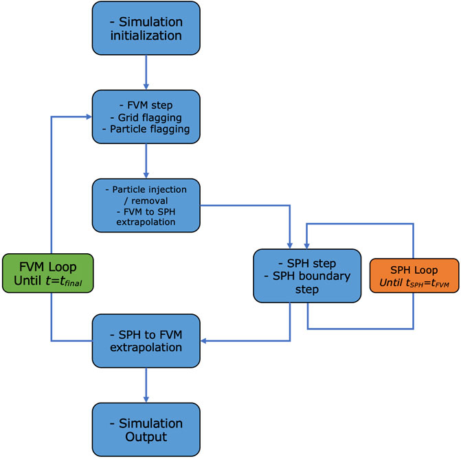
FIGURE 1. Depiction of the hybrid coupling algorithm’s simulation procedure. The green segment represents the FVM cycle, while the orange segment illustrates the SPH sub-cycle. Figure originally from [6].

FIGURE 2

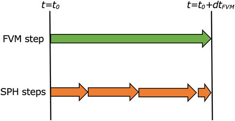
FIGURE 2. Illustration of the time stepping strategy for the Hybrid FVM-SPH simulation. The FVM time step maintains a constant size, while the SPH time step can vary and is generally smaller. The last SPH time step in the SPH sub-loop is adjusted to align with the FVM time. Figure originally from [6].

The hybrid simulation starts with the FVM and SPH simulations being initialized to a starting state. The fluid values and numerical parameters are loaded, and the domain and boundaries for both schemes are established. An SPH injection map is created based on the FVM mesh so that injected particles will be introduced in a regular pattern to prevent instabilities and oscillations in new particles. Hybrid simulation parameters are also set, including the size of SPH active and boundary regions around discontinuities.

The main loop begins with the FVM simulation moving forward one time step. The time step used is substantially larger than what is typically needed to resolve the shock since the SPH simulation is relied upon in these regions. The limiting factor is instead determined by the advancement in the shock in the SPH scheme. The FVM simulation must evolve fast enough such that SPH does not reach its boundary region before the FVM updates. A time step of around 1e-5 was used in both simulated problems. Once the FVM time step is completed, the gradients of the resulting field are calculated across the FVM cells, and those found to be higher than a predetermined threshold are marked for SPH modeling. A buffer region around the flagged cells is included in the SPH cells to account for the movement of the shocks, and a boundary region is established around all of these cells. Any cells that changed from unflagged to SPH active or boundary regions require new SPH particles, which are injected at locations determined by the injection map. Figure 3 provides a visual representation of these steps.

FIGURE 3

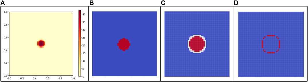
FIGURE 3. Illustration of the FVM flagging process: (A) Field values in FVM. (B) Cells with gradients surpassing a predefined threshold are identified. (C) Identified cells are designated as active SPH regions (in red), and the neighboring cells become boundary SPH regions (in white). (D) SPH injection map identifies zones (in red) for the addition of new SPH particles. Figure originally from [6].

Once new particles are injected, all particles are flagged based on whether they are in active SPH cells, boundary cells, or inactive cells. Any particles not marked as active or boundary cells are removed. The FVM values are interpolated to boundary SPH particles through a linear interpolation technique inspired by the Particle-in-Cell simulation method in plasma physics [42]:

$\begin{array}{l}\hfill f\left(x_i,y_i\right)=w_a{f}_a+w_b{f}_b+w_c{f}_c+w_d{f}_d\\ \hfill =\left(x_d-x_i\right)\left(y_i-y_d\right)f_a+\left(x_i-x_c\right)\left(y_i-y_c\right)f_b\\ \hfill +\left(x_b-x_i\right)\left(y_b-y_i\right)f_c+\left(x_i-x_a\right)\left(y_d-y_i\right)f_d\end{array}(23)$

A representation of the interpolation scheme is shown in Figure 4. In Equation 23, f corresponds to a chosen field value. The coupled fields include density, x- and y-velocities, and pressure, and energy. The i subscripts indicate the SPH particle x and y coordinates, whereas the a, b, c, and d subscripts represent the nearest four FVM cell centers as demonstrated in Figure 4. After interpolation, the field values of SPH boundary particles are stored so that values can be reverted after each SPH time step. This approach to SPH boundaries, fixing the particle positions and values for particles at the SPH domain’s edge, was significantly more efficient than using the built-in boundary approaches. Additionally, the simplicity and robustness of the approach allow for easy integration into the hybrid scheme, where complicated boundary configurations may form.

FIGURE 4

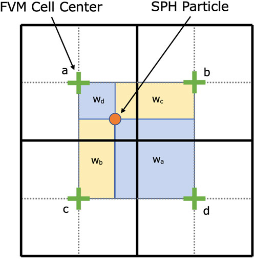
FIGURE 4. Illustration of the FVM-SPH interpolation method. The field value f is determined through 2D linear interpolation, in which the weights w_a, w_b, w_c, and w_d are applied to the respective fields at cells a, b, c, and d. Figure originally from [6].

The SPH simulation then moves forward one step in time. In previous work, the SPH time step was calculated using the CFL condition, where the time step chosen was proportional to the time it takes a particle to travel one particle smoothing length h. The smallest of these values, determined from each particle smoothing length and sound speed, was selected. This approach was not chosen as it added significant computational expense at each step because of the size of the problem and often did not produce accurate results. Instead, an empirical, parabolic time step relation was derived from the time steps used in the CTH reference simulations until 18 μs. After that, a fixed time step was used proportional to the discretization size.

After the SPH simulation time reaches the FVM time, active SPH particles’ values are interpolated to the FVM cells. Each particle’s field value is divided into the nearest four FVM cell centers, inversely proportional to the distance from each cell center, shown in Figure 4. Once all the particles’ values have been distributed, the value in each cell is weighted by the number of particles and their respective weight [6]:

$f_a=\frac{{\sum }_{i=1}^N{f}_i{w}_i}{{\sum }_{i=1}^N{w}_i}(24)$

For the N particles distributed to a given FVM cell a.

The SPH variables interpolated to the FVM mesh are in primitive form, so the conservative form variables are then calculated for the FVM mesh. The FVM boundaries at the edges of the domain are updated, and the simulation is prepared to begin the next step of the main simulation loop. The loop is repeated until the final simulation time is reached. All data is then stored, including FVM cell data, SPH particle data, and general simulation parameters, including runtime and initialization data.

The FVM and SPH methods used in the hybrid algorithm conserve mass, momentum, and energy through the simulation. Ensuring conservation of the coupling algorithm is critical for the stability and accuracy of the hybrid approach. In linearly interpolating values directly between particles and FVM cell centers, the interpolated values are conserved across interpolation steps. Mass and energy are directly interpolated between particles and cells, and as a result are strictly conserved. Momentum is not directly conserved as velocity is interpolated between particles. Future research may include direct interpolation of momentum to strictly ensure conservation, but the current approach was found to be stable and accurate for the examined problems.

While linearly interpolating values ensures conservation, the interpolation can be diffusive for regions with high gradients. To avoid diffusion, the interpolating boundary regions between cells and particles is separated from flagged regions by at minimum two FVM cells. Lower gradient regions not flagged by the hybrid algorithm can experience some diffusion, but it was not found to be significant enough in the examined problems to use an alternative interpolation approach.

5 Results

To evaluate the hybrid SPH methodology, the FVM, SPH, and hybrid approaches were applied to 1 kt and 10 kt blast simulations modeled in CTH. The problem was initialized as a 2D volume of air at standard atmospheric pressure and density, specifically 102 kPa and 1.225 kg/m³, respectively. The explosive was initiated by setting a cylindrical volume to a density of 1,000 kg/m³ and the pressure such that the total energy of the air inside the cylindrical volume equaled the required energies of 1 kt and 10 kt.

To fairly compare the FVM and SPH approaches with the hybrid approach, a variable domain size protocol was implemented that increased the size of each problem only when needed. Each problem began with a 10-m by 10-m domain until the shock wave from the explosive approached the edges. At that point, the data was saved to storage, and the simulation was re-initialized with a larger domain. The previous data was then loaded into the larger simulation and advanced forward in time until it became necessary to repeat the process. As the number of cells or particles is proportional to the area of the domain for a fixed discretization size, this technique saved a significant amount of time for the FVM and SPH simulations in the early stages, particularly because of the small timesteps needed at the start of the simulation.

A resolution corresponding to 20 cm was utilized in the FVM, SPH, and hybrid simulations. Testing with 10 and 5 cm resolutions led to significantly higher runtimes and memory issues encountered at earlier simulated times while providing minimal improvements in blast wave radius relative to the reference simulation. At 20 cm, the SPH simulation, utilizing a GSPH scheme, was able to approximately model the propagation of the shock wave found in the CTH simulation. Although the FVM simulation underperformed the SPH simulation, even at higher resolutions, the FVM code was selected to serve as an efficient, coarse model for the hybrid simulation.

At the start of the simulations, the initial timestep for all problems was set to 6.25e-11 s and 3.125e-11 s for the 1 kt and 10 kt problems, respectively. The growth in timestep was capped at a maximum value equal to the square of the number of simulated steps times the initial timestep until a simulated time of 18 μs:

$\mathrm{\Delta }{t}_{\mathit{max}}=\left\{\begin{array}{c}\mathrm{\Delta }{t}_{\mathit{initial}}*{\left(step\right)}^{2}if<18\mu s\hfill \\ \mathrm{\Delta }{t}_{\mathit{CFL}}else\hfill \end{array}\right\}(25)$

Beyond the prescribed time, the simulation determined the timestep via the CFL condition, although the calculated timesteps typically remained below 2 μs and 1 μs after the early stages once the shockwave had formed. The initial timestep size and maximum timestep growth were selected to ensure accuracy and stability at the start of the simulation, where the adaptive timesteps were found to be too large. The initial timestep and timestep growth mirrored those seen in the reference CTH simulation, although the growth in timesteps was smaller than in the CTH simulation.

The hybrid simulation required both a coarse FVM simulation and a fine SPH simulation to model the problem. An important parameter of the hybrid simulation was the ratio of the SPH to FVM resolution, previously denoted as $\beta =\frac{\mathrm{\Delta }{x}_{\mathit{SPH}}}{\mathrm{\Delta }{x}_{\mathit{FVM}}}$. Previous investigations determined an optimal value of β = 4, which was found to be comparable or faster than β = 2 and β = 8 in most cases, although the differences between each value were relatively small. Other important hybrid parameters included the number of active and boundary cells surrounding the SPH region; a value of one for each was found to be sufficient.

5.1 1 kt detonation

The 1 kt detonation was modeled using FVM, SPH, and the hybrid approach until 1 ms. Initial conditions and parameters used in the SPH and hybrid schemes for both the 1 kt and 10 kt blast simulations are shown in Table 1. Open boundary conditions are used at the edges of the domain. In the FVM and SPH simulations, the initial domain length was set to 10 m and increased by 5 m when the shockwave approached the boundaries until a size of 50 m. The domain then expanded by 10 m until a total length of 100 m, beyond which the simulation expanded by 25 m each time. As an aid for interpreting the 1D data, a 2D visualization of the results is shown in Figure 5. The hybrid simulation was initialized to 100 m from the beginning but with a coarse FVM mesh and a limited number of SPH particles only around the central explosive.

TABLE 1

TABLE 1. Initial Conditions and SPH parameters for the SPH and hybrid schemes in the 1 kt and 10 kt blast simulations. The kernel factor denotes particle size, g1 and g2 are numerical parameters used in the GSPH scheme implemented in [21], and γ is the ratio of specific heats. The explosive is initialized as a cylinder of uniform high pressure and high density air. Regions outside the initial radius are set to standard atmospheric pressure and density. The pressure and density of cells that contain regions both inside and out of the initial explosive radius are weighted by the area that in inside the radius.

FIGURE 5

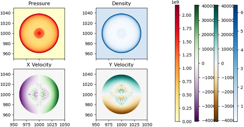
FIGURE 5. FVM results for 1 kt detonation in air at t = 1 ms.

The simulation runtimes for the FVM, SPH, and hybrid simulations are displayed in Figure 6. The hybrid approach is more efficient than the FVM or SPH approaches after early time and is approximately an order of magnitude faster than both near the end of the simulation. The steep rise in runtime seen in the FVM and SPH simulations is largely due to the increasing domain size as the shockwave propagates, necessitating additional cells and particles. At early times, the hybrid method does not have any advantage since the domains are small in all cases, and the majority of the runtime is due to the number of timesteps rather than the number of cells or particles.

FIGURE 6

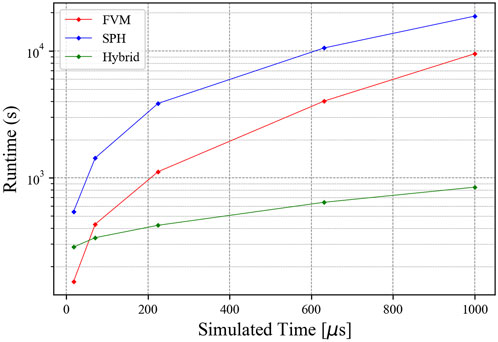
FIGURE 6. Simulation runtimes for 1 kt blast simulations using FVM, SPH, and hybrid approaches.

Simulation runtime speedup over the SPH simulation is shown in Figure 7. The speedup is found by dividing each runtime at every simulation time output by the SPH runtime and inverting the result. At early times, the hybrid result is comparable to the FVM result but continues to rise to 22.3x over the course of the simulation. The FVM simulation is faster than the SPH simulation at all output times, but the FVM speedup reduces as the simulation progresses.

FIGURE 7

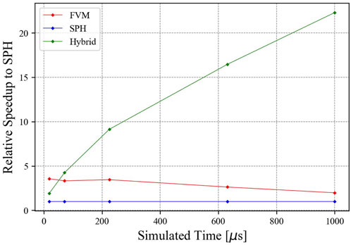
FIGURE 7. Relative simulation runtime speedup over the SPH simulation for the 1 kt blast simulation.

One-dimensional lineouts of density at select times through the center of the domain are shown in Figure 8. Times were selected to show the formation and propagation of the shockwave in each approach. At 18 μs, FVM significantly overestimates peak density, while SPH and hybrid approaches underestimate density relative to the CTH simulation. As time progresses, the FVM density falls closer to the reference simulation value but propagates faster. The SPH and hybrid simulation shockwaves initially lag behind the reference simulation shockwave and underestimate density, but they converge at a later time.

FIGURE 8

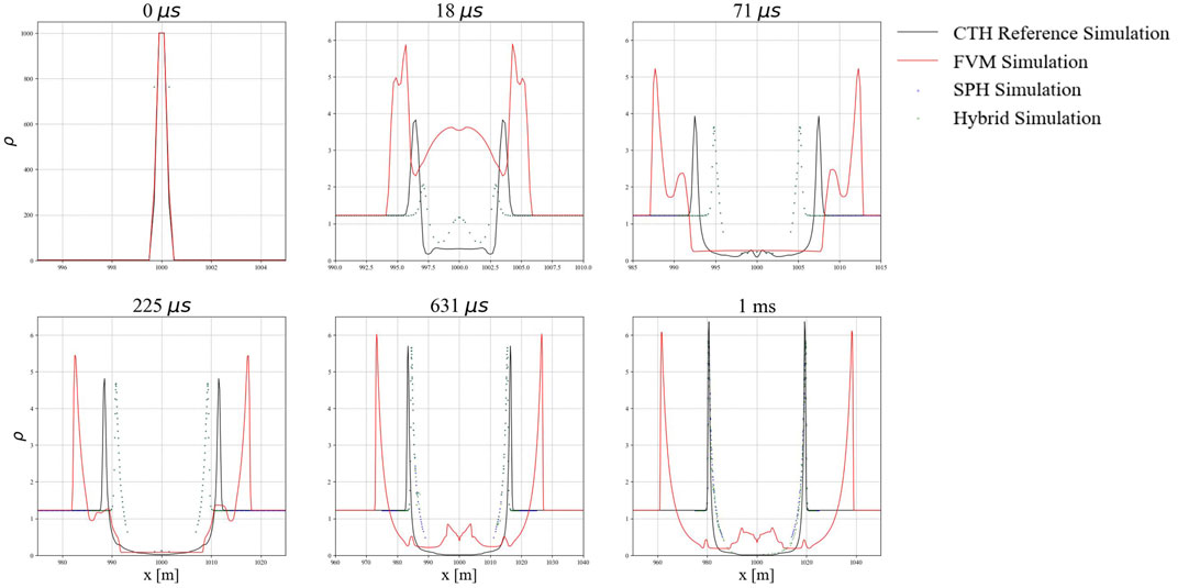
FIGURE 8. Simulations results for center-line density for a 1 kt blast simulation at t = 1 ms for the CTH reference simulation and using FVM, SPH, and hybrid approaches.

The peak density and shockwave radius for each approach and the reference simulation are displayed in Figure 9. Given that the SPH and hybrid simulations are essentially the same but with a smaller domain in the hybrid simulation, the results overlap for most of the recorded times but exhibit some slight variation for peak density. The SPH and hybrid peak densities are initially below the reference simulation before converging and then diverging below again around 1 ms. The FVM simulation overestimates peak density until the end of the simulation, at which point it falls below the reference simulation. The SPH and hybrid simulation closely follow the reference blast radius initially before overshooting, while the FVM simulation overestimates the blast radius at all simulation times.

FIGURE 9

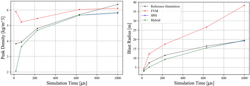
FIGURE 9. Peak shockwave density and radius for a 1 kt blast simulation at t = 1 ms for the CTH reference simulation and using FVM, SPH, and hybrid approaches.

5.2 10 kt detonation

The 1 kt detonation was modeled using each approach until 1 ms. The initial conditions for the 10 kt problem are given in Table 1. Open boundary conditions are used at the edges of the domain. In the FVM and SPH simulations, the initial domain length was set to 10 m and was increased the same amount as in the 1 kt simulation. However, the shockwave propagated faster in the 10 kt simulation, resulting in a larger and more rapidly expanding domain. As an aid for interpreting the 1D data, a 2D visualization of the results is shown in Figure 10. The hybrid simulation was initialized to 100 m from the beginning, featuring a coarse FVM mesh and SPH particles in the center, similar to the 1 kt setup.

FIGURE 10

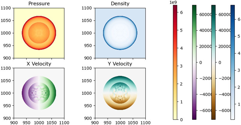
FIGURE 10. FVM results for 10 kt detonation in air at t = 1 ms.

The simulation runtimes for the FVM, SPH, and hybrid simulations are displayed in Figure 11. The hybrid approach is more efficient than the FVM or SPH approaches. Similar performance behaviors over simulated runtime are observed across each approach but with a longer overall runtime. The hybrid approach remains approximately an order of magnitude more efficient than the FVM or SPH approaches, while the FVM approach has performance approaching that of the SPH approach at 631 μs and 1 ms as it overestimates the propagation of the shockwave and requires a larger domain.

FIGURE 11

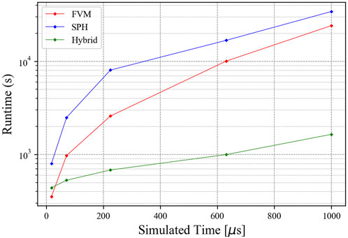
FIGURE 11. Simulation runtimes for 10 kt blast simulations using FVM, SPH, and hybrid approaches.

Simulation runtime speedup over the SPH simulation is shown in Figure 12. At early times, the hybrid result is comparable to the FVM result but quickly rises to a 11.8x speedup over the SPH simulation. The rate of speedup decreases moderately but the speedup continues to rise to 20.9x by the end of the simulation. The FVM simulation moderately faster than the SPH simulation at early times but the speedup reduces to be relatively close to SPH by the end of the simulation.

FIGURE 12

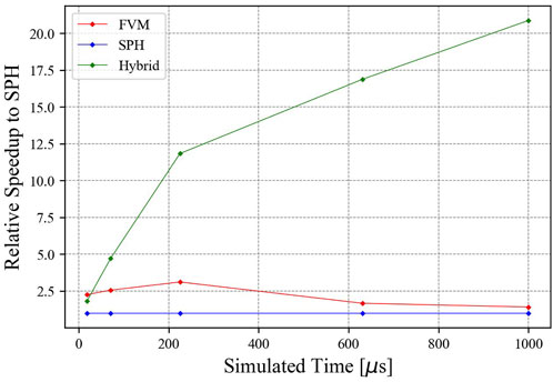
FIGURE 12. Relative simulation runtime speedup over the SPH simulation for the 10 kt blast simulation.

One-dimensional lineouts of density at select times through the center of the domain are shown in Figure 13. The FVM approach again overestimates the speed of the shockwave. However, the magnitude of the peak density remains below the reference simulation at all output times. The SPH and hybrid approaches similarly underestimate density but are more accurate in determining the location of the shockwave.

FIGURE 13

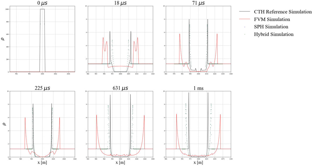
FIGURE 13. Simulations results for center-line density for a 10 kt blast simulation at t = 1 ms for the CTH reference simulation and using FVM, SPH, and hybrid approaches.

The peak density and shockwave radius for each approach and the reference simulation are displayed in Figure 14. The reference simulation predicts a higher peak density than each approach. Interestingly, the reference simulation predicts an increase in peak density that occurs between 225 and 631 μs, which is not seen in the FVM, SPH, or hybrid approaches. The SPH and hybrid approaches overestimate the shockwave radius, while the FVM radius diverges from the reference simulation more rapidly than in the 1 kt problem.

FIGURE 14

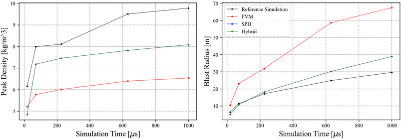
FIGURE 14. Peak shockwave density and radius for a 10 kt blast simulation at t = 1 ms for the CTH reference simulation and using FVM, SPH, and hybrid approaches.

6 Discussion and future work

The hybrid SPH method discussed here offers a distinct approach to blast simulations, presenting potential applications beyond conventional mesh-based simulations. The merits of the Lagrangian method, such as modeling various materials affected by a blast and tracking deformation and fracturing, can be achieved without the usual inefficiency of meshless methods. By confining the spread of SPH particles to the areas surrounding shockwaves, we have improved the performance tenfold while preserving the characteristics of a shockwave as modeled by SPH. This presents a promising avenue for enhancing the performance of SPH-based blast investigations in scenarios where vast regions exhibit no significant gradients.

Given that we used Python frameworks to evaluate each individual approach and construct the hybrid approach, there are certain limitations to the evaluation undertaken here. Python is not typically chosen for its efficiency, and numerous optimizations can be applied to each of the frameworks used in this study. Many faster versions of FVM and SPH, available in compiled languages, can offer a more accurate assessment of the true speed of these methods; however, these investigations are left to future researchers. Nonetheless, the development and testing of the hybrid SPH method for compressible blast simulations, which, according to the literature surveyed, has only been recently explored [33], carries intrinsic value.

The hybrid SPH method provides an alternative approach to AMR for grid-based simulations with new applications. Of particular interest in blast simulations is the interaction of shockwaves with structures and the surrounding environment. As seen in previous hybrid-SPH simulations of water and incompressible fluids, hybrid-SPH simulations for compressible fluids can facilitate the streamlined modeling of several phenomena in a given problem, which typically involves varying characteristics and often different physics. Moreover, the straightforward interaction between SPH-modeled fluids and SPH-modeled solids enables easy fluid-structure modeling, making it more accessible to a wider range of researchers. In addition to fluid structure interaction problems, future work includes extending and testing the hybrid approach in three dimensions and implementing and evaluating parallel hybrid SPH simulations. Such extensions require switching to an alternative FVM solver, as Pyro2 does not include parallelization capability.

7 Conclusion

In conclusion, this work has introduced and demonstrated the effectiveness of a hybrid FVM-SPH scheme for capturing shocks in compressible fluids. The method was successfully applied to 1 kt and 10 kt blast simulations. The proposed hybrid approach places SPH particles in areas with high gradients, interpolating field values between FVM and SPH through boundary particles and cells. This method was tested for accuracy and computational efficiency against traditional SPH methods and FVM methods without adaptive mesh refinement capability. Notably, it demonstrated a tenfold increase in performance over traditional methods while retaining the accuracy and character of an SPH simulation.

This innovative strategy could improve the way researchers approach blast simulations, as it combines the advantages of both FVM and SPH methods. The hybrid approach, by selectively utilizing SPH particles only in regions of high gradients, avoids the general inefficiencies associated with meshless methods. As a result, the flexibility and diverse application potential of the Lagrangian method can be harnessed without the corresponding performance drawbacks. Furthermore, the dramatic performance enhancement without sacrificing accuracy opens up new avenues for complex blast simulations, especially in scenarios involving large regions without significant gradients. Therefore, this work contributes a novel perspective to the existing body of research, potentially aiding further explorations in the realm of computational blast simulations.

Data availability statement

The datasets presented in this study can be found in online repositories. The names of the repository/repositories and accession number(s) can be found below: https://github.com/myerscon/hybridSPH/.

Author contributions

CM: Conceptualization, Data curation, Formal Analysis, Investigation, Methodology, Software, Visualization, Writing–original draft. JM: Data curation, Investigation, Validation, Writing–review and editing. TP: Conceptualization, Resources, Supervision, Writing–review and editing. CP: Conceptualization, Funding acquisition, Project administration, Resources, Supervision, Writing–review and editing.

Funding

The author(s) declare financial support was received for the research, authorship, and/or publication of this article. The authors gratefully acknowledge the support of the Laboratory Directed Research and Development (LDRD) program at Sandia National Laboratories. Sandia National Laboratories is a multi-mission laboratory managed and operated by National Technology and Engineering Solutions of Sandia, LLC., a wholly owned subsidiary of Honeywell International, Inc., for the U.S. Department of Energy’s National Nuclear Security Administration under contract DE-NA0003525. The views expressed in the article do not necessarily represent the views of the U.S. Department of Energy or the United States Government. The authors additionally acknowledge Mike Owen at Lawrence Livermore National Laboratory for guidance in the early stages of the development of the hybrid FVM-SPH method.

Conflict of interest

The authors declare that the research was conducted in the absence of any commercial or financial relationships that could be construed as a potential conflict of interest.

Publisher’s note

All claims expressed in this article are solely those of the authors and do not necessarily represent those of their affiliated organizations, or those of the publisher, the editors and the reviewers. Any product that may be evaluated in this article, or claim that may be made by its manufacturer, is not guaranteed or endorsed by the publisher.

References

1. Delmastro AC, Spriggs GD. Light output and thermal blast analysis of nuclear fireballs. Tech. rep. United States (2018).

CrossRef Full Text | Google Scholar

2. Anderson JD. Discretization of partial differential equations. In: Computational fluid dynamics: an introduction. London: Springer (2008). p. 100–3.

Google Scholar

3. Berger MJ, Colella P. Local adaptive mesh refinement for shock hydrodynamics. J Comput Phys (1989) 82(1):64–84. doi:10.1016/0021-9991(89)90035-1

CrossRef Full Text | Google Scholar

4. Salas MD. Shock fitting method for complicated two-dimensional supersonic flows. AIAA J (1976) 14(5):583–8. doi:10.2514/3.61399

CrossRef Full Text | Google Scholar

5. Myers C, Palmer C, Palmer T. A coupled smoothed particle hydrodynamics-finite volume approach for shock capturing in one-dimension. Heliyon (2023) 9(7):e17922. doi:10.1016/j.heliyon.2023.e17922

PubMed Abstract | CrossRef Full Text | Google Scholar

6. Myers C, Palmer T, Palmer C. A hybrid finite volume-smoothed particle hydrodynamics approach for shock capturing applications. Comput Methods Appl Mech Eng (2023) 417:116412. doi:10.1016/j.cma.2023.116412

CrossRef Full Text | Google Scholar

7. Yao X, Huang D. Coupled pd-sph modeling for fluid-structure interaction problems with large deformation and fracturing. Comput structures (2022) 270:106847–66. doi:10.1016/j.compstruc.2022.106847

CrossRef Full Text | Google Scholar

8. Gharehdash S, Barzegar M, Palymskiy IB, Fomin PA. Blast induced fracture modelling using smoothed particle hydrodynamics. Int J Impact Eng (2020) 135:103235–56. doi:10.1016/j.ijimpeng.2019.02.001

CrossRef Full Text | Google Scholar

9. Zhang Z, Liu M. Smoothed particle hydrodynamics with kernel gradient correction for modeling high velocity impact in two- and three-dimensional spaces. Eng Anal Boundary Elem (2017) 83:141–57. doi:10.1016/j.enganabound.2017.07.015

CrossRef Full Text | Google Scholar

10. Gou J, Yuan X, Su X. A high-order element based adaptive mesh refinement strategy for three-dimensional unstructured grid. Int J Numer Methods Fluids (2017) 85(9):538–60. doi:10.1002/fld.4397

CrossRef Full Text | Google Scholar

11. Colella P. Multidimensional upwind methods for hyperbolic conservation laws. J Comput Phys (1990) 87(1):171–200. doi:10.1016/0021-9991(90)90233-q

CrossRef Full Text | Google Scholar

12. LeVeque RJ. Gas dynamics and the euler equations. In: Finite volume methods for hyperbolic problems. New York: Cambridge University Press (2002). p. 291–310.

Google Scholar

13. Liu GR, Liu MB. Smoothed particle hydrodynamics: a meshfree particle method. New Jersey: World Scientific (2003).

Google Scholar

14. Balsara DS. Von neumann stability analysis of smoothed particle hydrodynamics—suggestions for optimal algorithms. J Comput Phys (1995) 121(2):357–72. doi:10.1016/s0021-9991(95)90221-x

CrossRef Full Text | Google Scholar

15. Liu M, Liu G, Lam K. Constructing smoothing functions in smoothed particle hydrodynamics with applications. J Comput Appl Math (2003) 155(2):263–84. doi:10.1016/s0377-0427(02)00869-5

CrossRef Full Text | Google Scholar

16. Gingold RA, Monaghan JJ. Smoothed particle hydrodynamics: theory and application to non-spherical stars. Monthly notices R Astronomical Soc (1977) 181(3):375–89. doi:10.1093/mnras/181.3.375

CrossRef Full Text | Google Scholar

17. Monaghan J, Gingold R. Shock simulation by the particle method sph. J Comput Phys (1983) 52(2):374–89. doi:10.1016/0021-9991(83)90036-0

CrossRef Full Text | Google Scholar

18. Sigalotti LDG, Daza D, Donoso A. Modelling free surface flows with smoothed particle hydrodynamics. Condensed matter Phys (2006) 9(2):359–66. doi:10.5488/cmp.9.2.359

CrossRef Full Text | Google Scholar

19. Price DJ. Smoothed particle hydrodynamics and magnetohydrodynamics. J Comput Phys (2012) 231(3):759–94. doi:10.1016/j.jcp.2010.12.011

CrossRef Full Text | Google Scholar

20. Inutsuka S. Reformulation of smoothed particle hydrodynamics with riemann solver. J Comput Phys (2002) 179(1):238–67. doi:10.1006/jcph.2002.7053

CrossRef Full Text | Google Scholar

21. Puri K, Ramachandran P. A comparison of sph schemes for the compressible euler equations. J Comput Phys (2014) 256:308–33. doi:10.1016/j.jcp.2013.08.060

CrossRef Full Text | Google Scholar

22. Murante G, Borgani S, Brunino R, Cha SH. Hydrodynamic simulations with the Godunov smoothed particle hydrodynamics. Monthly Notices R Astronomical Soc (2011) 417(1):136–53. doi:10.1111/j.1365-2966.2011.19021.x

CrossRef Full Text | Google Scholar

23. Fox RW. Introduction to fluid mechanics. John Wiley and Sons (1992).

Google Scholar

24. Fourey G, Hermange C, Le Touzé D, Oger G. An efficient fsi coupling strategy between smoothed particle hydrodynamics and finite element methods. Comput Phys Commun (2017) 217:66–81. doi:10.1016/j.cpc.2017.04.005

CrossRef Full Text | Google Scholar

25. Chen C, Shi WK, Shen YM, Chen JQ, Zhang AM. A multi-resolution sph-fem method for fluid–structure interactions. Comput Methods Appl Mech Eng (2022) 401:115659. doi:10.1016/j.cma.2022.115659

CrossRef Full Text | Google Scholar

26. Dinçer AE, Demir A, Bozkuş Z, Tijsseling AS. Fully coupled smoothed particle hydrodynamics-finite element method approach for fluid–structure interaction problems with large deflections. J Fluids Eng (2019) 141(8). doi:10.1115/1.4043058

CrossRef Full Text | Google Scholar

27. Hermange C, Oger G, Le Chenadec Y, Le Touzé D. A 3d sph–fe coupling for fsi problems and its application to tire hydroplaning simulations on rough ground. Comput Methods Appl Mech Eng (2019) 355:558–90. doi:10.1016/j.cma.2019.06.033

CrossRef Full Text | Google Scholar

28. Afrasiabi M, Roethlin M, Wegener K. Thermal simulation in multiphase incompressible flows using coupled meshfree and particle level set methods. Comput Methods Appl Mech Eng (2018) 336:667–94. doi:10.1016/j.cma.2018.03.021

CrossRef Full Text | Google Scholar

29. Kumar P, Yang Q, Jones V, McCue-Weil L. Coupled sph-fvm simulation within the openfoam framework. Proced IUTAM (2015) 18:76–84. doi:10.1016/j.piutam.2015.11.008

CrossRef Full Text | Google Scholar

30. Marrone S, Di Mascio A, Le Touzé D. Coupling of smoothed particle hydrodynamics with finite volume method for free-surface flows. J Comput Phys (2016) 310:161–80. doi:10.1016/j.jcp.2015.11.059

CrossRef Full Text | Google Scholar

31. Chiron L, Marrone S, Di Mascio A, Le Touzé D. Coupled sph–fv method with net vorticity and mass transfer. J Comput Phys (2018) 364:111–36. doi:10.1016/j.jcp.2018.02.052

CrossRef Full Text | Google Scholar

32. Xu Y, Yang G, Zhu Y, Hu D. A coupled sph–fvm method for simulating incompressible interfacial flows with large density difference. Eng Anal Boundary Elem (2021) 128:227–43. doi:10.1016/j.enganabound.2021.04.005

CrossRef Full Text | Google Scholar

33. Tsuji P, Puso M, Spangler CW, Owen JM, Goto D, Orzechowski T. Embedded smoothed particle hydrodynamics. Comput Methods Appl Mech Eng (2020) 366:113003. doi:10.1016/j.cma.2020.113003

CrossRef Full Text | Google Scholar

34. Vacondio R, Altomare C, De Leffe M, Hu X, Le Touzé D, Lind S, et al. Grand challenges for smoothed particle hydrodynamics numerical schemes. Comput Part Mech (2021) 8(3):575–88. doi:10.1007/s40571-020-00354-1

CrossRef Full Text | Google Scholar

35. Harpole A, Zingale M, Hawke I, Chegini T. Pyro: a framework for hydrodynamics explorations and prototyping. J Open Source Softw (2019) 4(34):1265. doi:10.21105/joss.01265

CrossRef Full Text | Google Scholar

36. Lam SK, Pitrou A, Seibert S. Numba: a llvm-based python jit compiler. In: Proceedings of the second workshop on the LLVM compiler infrastructure in HPC. New York, NY, USA: Association for Computing Machinery (2015). p. 6.

Google Scholar

37. Ramachandran P, Bhosale A, Puri K, Negi P, Muta A, Dinesh A, et al. Pysph: a python-based framework for smoothed particle hydrodynamics. ACM Trans Math Softw (2021) 47(4):1–38. doi:10.1145/3460773

CrossRef Full Text | Google Scholar

38. Behnel S, Bradshaw R, Citro C, Dalcin L, Seljebotn DS, Smith K. Cython: the best of both worlds. Comput Sci Eng (2010) 13(2):31–9. doi:10.1109/mcse.2010.118

CrossRef Full Text | Google Scholar

39. Klöckner A, Pinto N, Lee Y, Catanzaro B, Ivanov P, Fasih A. Pycuda and pyopencl: a scripting-based approach to gpu run-time code generation. Parallel Comput (2012) 38(3):157–74. doi:10.1016/j.parco.2011.09.001

CrossRef Full Text | Google Scholar

40. Sigalotti LDG, López H, Donoso A, Sira E, Klapp J. A shock-capturing sph scheme based on adaptive kernel estimation. J Comput Phys (2006) 212(1):124–49. doi:10.1016/j.jcp.2005.06.016

CrossRef Full Text | Google Scholar

41. McGlaun J, Thompson S, Elrick M. Cth: a three-dimensional shock wave physics code. Int J Impact Eng (1990) 10(1):351–60. doi:10.1016/0734-743x(90)90071-3

CrossRef Full Text | Google Scholar

42. Birdsall CK. Plasma physics via computer simulation. Boca Raton, FL: CRC Press (1985).

Google Scholar