Enabling unstructured-mesh computation on massively tiled AI processors: An example of accelerating in silico cardiac simulation

1 Introduction

Real-world problems of computational physics often involve irregularly shaped solution domains, which require unstructured computational meshes [1] to accurately resolve them. The resulting numerical couplings between the entities of an unstructured mesh are irregular; thus, during the implementation of unstructured-mesh computations, irregular and indirectly-indexed accesses to arrays of numerical values are unavoidable. With respect to performance, there arise several challenges. First, irregular and indirect accesses to array entries are prohibitive for achieving the full speed of a standard memory system [2]. Second, for using a distributed-memory parallel platform, explicit partitioning of an unstructured mesh is required, which is considerably more difficult than partitioning a structured mesh [3]. Third, there currently exists no universal solution that ensures perfect quality of the partitioned sub-meshes. One specific problem inside the latter challenge is associated with the so-called halo regions. That is, the sub-meshes that arise from non-overlapping decomposition need to be expanded with one or several extra layers of mesh entities, which constitute a halo region of each sub-mesh. These halo regions will be used for facilitating the necessary information exchange between the sub-meshes. However, most of the partitioning strategies are incapable of producing an even distribution of the halo regions leading to imbalanced volumes of communication between the sub-meshes and different memory footprints of the sub-meshes.

One particular trend of the latest hardware development requires new attention to the abovementioned challenges. Namely, we have recently seen the arrival of processors with a huge number of small cores sharing no device-level memory. The most prominent examples are the wafer-scale engine (WSE) from Cerebras [4] and the intelligence processing unit (IPU) from Graphcore [5]. For example, the second-generation WSE-2 is a chip that consists of 2.6 trillion transistors and houses 850,000 cores. The MK2 GC200 IPU is smaller in scale, but still has 59.4 billion transistors and 1,472 cores. A common design theme of these processors is that there is no device-level memory that is shared among the cores. Instead, each core has its private SRAM and the aggregate on-chip memory bandwidth is staggeringly high at 20 PB/s for WSE-2 [4] and 47.5 TB/s for MK2 GC200 IPU [5]. Although these processors are primarily designed for AI workloads, the available aggregate memory bandwidth is appealing to many tasks of scientific computing for which the performance relies on the speed of moving data in and out of the memory system. Storing data directly in the SRAM can avoid many “data locality problems” that are typically associated with the multi-leveled caching system found on standard processor architectures. However, we need to remember that a core with its private SRAM, termed as a tile, constitutes the basic work unit on WSE-2 or IPU. This leads to higher requirements related to partitioning unstructured-mesh computations, both due to the huge number of available tiles and because all the data needed by each tile must fit into its limited local SRAM. In addition, enabling necessary communication and coordination between the sub-meshes (i.e., the tiles) requires a new way of programming, unlike using the standard MPI library [6].

Motivated by the extreme computing power that theoretically can be delivered by the massively tiled AI processors, researchers have recently started applying these AI processors to “traditional” computational science. For example, Graphcore IPUs have been used for particle physics [7], computer vision [8], and graph processing [9, 10]. Regarding mesh-based computations for numerically solving partial differential equations (PDEs), the current research effort is limited to porting stencil methods that are based on uniform meshes and finite difference discretization. This limitation applies to both Cerebras WSE [11, 12] and Graphcore IPUs [13, 14]. To the best of our knowledge, the subject of porting unstructured-mesh computation to massively tiled processors has not yet been addressed.

This paper aims to investigate how to program massively tiled processors for unstructured mesh computations. The Graphcore IPU, which is a relatively mature AI processor, is adopted as the hardware testbed. Specifically, we study the performance impact of partitioning an unstructured mesh into huge numbers of sub-meshes, as well as how to facilitate communication between the sub-meshes through special IPU programming. Another topic of generic characteristic to study in this paper is the achievable performance and accuracy of evaluating special mathematical functions, such as exp, log, and sqrt, on the IPU. As a real-world application of computational physics, we port an existing code that simulates the electrophysiology inside the heart ventricles, which need to be resolved by high-resolution 3D unstructured meshes. Our work, thus, makes the following contributions:

• We present a new programming scheme, based on Graphcore’s Poplar software stack, for implementing parallel sparse matrix-vector multiply (SpMV) operations that arise from partitioning unstructured meshes.

• We study the impact of mesh partitioning on the size of halo regions and the associated memory footprints, as well as the performance loss due to the communication overhead. These will be investigated for both single- and multi-IPU scenarios.

• We benchmark, in detail, the achievable accuracy and speed of some chosen mathematical functions on IPUs using single precision.

• We demonstrate how a real-world application of computational physics, namely, simulating cardiac electrophysiology on 3D unstructured meshes, can utilize the computing power of IPUs.

• We also address the subject of performance analysis of unstructured-mesh computations on IPUs.

It is remarked that the chosen existing code numerically solves a widely used mathematical model in computational electrophysiology. The choice is also motivated by the fact that the performance of the code on GPUs has been carefully optimized and studied in [15], thus providing a comparison baseline for this paper where one of the research subjects is the achievable performance of unstructured mesh computations on IPUs. No new numerical algorithm will be introduced in this paper. Specifically, cell-centered finite volume discretization in space and explicit integration in time (used by the existing code, and more details can be found in Section 3) will continue to be used. The readers will recognize two familiar computational kernels, namely, parallel SpMV operations arising from unstructured meshes, and explicit integration of systems of non-linear ordinary differential equations (ODEs). The findings of this paper, regarding both the programming details needed to enable inter-tile communication on IPUs and the achievable performance, will thus be applicable beyond the domain of computational electrophysiology.

The remainder of this paper is organized as follows. Section 2 gives a brief introduction to the mathematical model considered, whereas Section 3 explains the numerical strategy and parallelization of the existing simulator. Section 4 focuses on the new programming details required for using the IPU. Numerical accuracy is considered in Sections 5 and 6. The former measures the general floating-point accuracy of the IPU, while the latter tests the fidelity of the simulation using an established benchmark. Section 7 presents the measured performance of our IPU implementation, together with a comparison with the GPU counterpart. The impact of imbalanced halo region distribution is also investigated. Section 8 concludes the paper.

2 Monodomain model of cardiac electrophysiology

The increase in computing power over the past decades has facilitated the use of computer simulations to better understand cardiac pathologies. One of the most important cardiac processes is the propagation of the electrical signals, which triggers the contraction of the heart muscle. This process of electrophysiology, in its simplest form, can be mathematically described as a reaction–diffusion system using the following monodomain model (see, e.g., [16]):

$\frac{\partial v}{\partial t}+\chi I_{\text{ion}}\left(t,v,\vec{s}\right)=\nabla \cdot \left(M\nabla v\right).(1)$

In the above model, v (x, y, z, t) denotes the transmembrane potential and is mathematically considered as a time-dependent 3D field, M (x, y, z) is a conductivity tensor field describing the space-varying cardiac muscle structure, χ is the ratio of the cell membrane area to the cell volume, and $I_{\text{ion}}(t,v,\vec{s})$ denotes the total ionic current across the cell membrane. Here, $\vec{s}(t)$ denotes a vector of state variables (apart from v) that also contributes to the evolvement of I_ion at each spatial point, where the evolution of $\vec{s}$ is governed by a system of ODEs (see below).

Despite its simplicity, the monodomain model (1) is frequently used by researchers to capture the main features of the signal propagation, especially over the entire heart. Numerically, this reaction–diffusion system is often solved using an operator splitting method to decouple the reaction term, $\chi I_{\text{ion}}(t,v,\vec{s})$, from the diffusion term, ∇ ⋅ (M∇v). The reaction part of the monodomain model is then formulated as a system of non-linear ODEs.

$\frac{\mathrm{d}v}{\mathrm{d}t}=-\chi I_{\text{ion}}\left(t,v,\vec{s}\right),(2)$

$\frac{\mathrm{d}\vec{s}}{\mathrm{d}t}=\vec{f}\left(t,v,\vec{s}\right).(3)$

This ODE system needs to be individually solved on each mesh entity of a computational grid. The diffusion part of the monodomain model is, thus, a linear 3D PDE as follows:

$\frac{\partial v}{\partial t}=\nabla \cdot \left(M\nabla v\right).(4)$

This PDE needs to be solved involving all the discrete v values in a computational grid.

In this paper, the ten Tusscher–Panfilov model (TP06, see [17]) is used for modeling I_ion, where the entire ODE system (2–3) involves v and 18 state variables. These state variables include various ionic currents and the so-called gating variables. Special math functions, such as exp, are heavily used in the ODEs. The source code of a straightforward implementation of the specific ODE system can be found in [18]. Furthermore, the TP06 model prescribes different parameters for three types of cardiac cells located in the epicardium (outer layer), the myocardium (middle layer), and the endocardium (inner layer) of the muscle wall in the cardiac ventricles.

3 Numerical strategy and distributed-memory parallelization

3.1 Unstructured tetrahedral meshes

To sufficiently resolve the irregular shapes inside a heart, we adopt unstructured tetrahedral meshes. The adopted bi-ventricular meshes are based on the dataset published by Martinez–Navarro et al. (see [19]) and the LDRB algorithm (see [20]) for determining muscle fiber directions. We have used transversely isotropic conductivity tensors such that the conductivity only depends on the longitudinal fiber direction, that is, parallel to the muscle fibers. Two realistic bi-ventricular meshes have been used for the numerical experiments to be presented later in this paper. The heart04 mesh has, in total, 3,031,704 tetrahedrons and a characteristic length of 0.4 mm, whereas the finer heart05 mesh has, in total, 7,205,076 tetrahedrons and a characteristic length of 0.3 mm. Figure 1 shows a simulated activation map of heart04 where a stimulus is applied initially to the apex of the left ventricle.

FIGURE 1

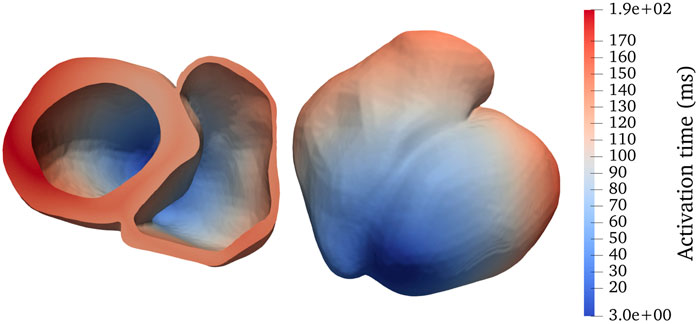
FIGURE 1. Activation map for a realistic bi-ventricular mesh, named heart04, with a stimulus applied initially to the apex of the left ventricle (darkest blue). The panels show two different viewing angles of the same mesh.

3.2 Discretization of the ODE systems

The non-linear ODE system (2–3) needs to be individually solved per tetrahedron. We follow previous studies [21, 22] in using an augmented forward Euler scheme, where one of the state variables (the so-called m gate) is integrated using the Rush–Larsen method [23] for improved numerical stability. That is, the other 17 state variables and v are explicitly integrated by the standard forward Euler scheme. In order to obtain sufficient accuracy, we use a time step Δt_ODE = 20  µs for the ODE system (2–3).

3.3 Discretization of the diffusion equation

The numerical solver for the diffusion equation (4) is based on cell-centered finite volume discretization in space and explicit integration in time [24, 25]. There exist other numerical strategies that are based on finite element discretization in space and/or implicit integration in time. We will provide a discussion in Section 8. The resulting computational stencil from the cell-centered finite volume discretization covers the four direct neighboring tetrahedrons plus the 12 second-tier neighbors such that the computational formula per tetrahedron depends on its 16 neighbors in addition to itself. This can be expressed straightforwardly as an SpMV operation:

${\vec{v}}_{n+1}=Z{\vec{v}}_n,(5)$

where the vectors ${\vec{v}}_{n+1}$ and ${\vec{v}}_n$ contain the numerical solutions at t = (n + 1)Δt_PDE and t = nΔt_PDE, respectively. Each value of vectors ${\vec{v}}_{n+1}$ or ${\vec{v}}_n$ is the numerical approximation of the transmembrane potential v at the center of a tetrahedron (which will also be called a cell in the remaining text). The matrix Z has a dense diagonal, and each row, corresponding to a specific tetrahedron, has up to 16 off-diagonal non-zero entries. The column positions of these non-zero entries are irregular due to the unstructured tetrahedral mesh.

The number of tetrahedrons of the 3D unstructured mesh is denoted by N. The diagonal of Z is stored as a separate 1D array, D, of length N, whereas the off-diagonal entries are stored in the ELLPACK format (see [26]) with 16 values per row. This results in two 2D arrays each with N × 16 entries: A contains the non-zero floating-point values in the off-diagonal part of matrix Z, and I contains the corresponding column indices.

As is common for explicit methods, the entries of Z impose a limit on how large the PDE time step Δt_PDE can be chosen without giving rise to numerical instability. When the criterion on Δt_PDE is much stricter than that on the ODE time step Δt_ODE, we use multi-stepping, meaning that p PDE steps with ${\mathrm{\Delta }t}_{\text{PDE}}=\frac{{\mathrm{\Delta }t}_{\text{ODE}}}{p}$ are executed for each ODE step. Otherwise, if the accuracy-determined value of Δt_ODE is roughly the same as the stability-determined value of Δt_PDE, the minimum of the two is used for solving both parts of the monodomain model.

3.4 Distributed-memory parallelization

On distributed-memory architectures, we need to partition the unstructured tetrahedral mesh in such a manner that the computation is evenly distributed among the hardware units, for example, the GPUs on a cluster or the tiles within an IPU. Furthermore, partitioning should ideally lead to a minimal communication volume to allow for scaling of the parallelized simulator. Specifically, we first construct an undirected graph based on the cell connectivity of the tetrahedral mesh and then use a graph partitioner (e.g., from the METIS library [27]) to create a partition that attempts to minimize the total communication volume within the constraints of a given maximal work imbalance ratio.

With respect to parallelizing the SpMV operation (5) that constitutes the computation of each PDE step, the non-overlapping sub-meshes that are produced by the graph partitioner dictate how the rows of the sparse matrix Z are distributed among the hardware units (such as the tiles within an IPU). Also, the input vector ${\vec{v}}_n$ that is to be multiplied with Z needs to be partitioned accordingly. On each hardware unit, besides its non-overlapping partition of ${\vec{v}}_n$, additional halo values of ${\vec{v}}_n$ need to be included. These halo values represent the needed contributions from the neighboring partitions; see Section 1. Before a distributed-memory parallel SpMV is executed, the halo values must be communicated from the neighbors. In return, some values within each non-overlapping partition of ${\vec{v}}_n$ are needed as halo values on the neighbors, so these values must be communicated to the neighbors.

4 Porting to the Graphcore IPU

We have chosen an existing code as the starting point, which is described in [15, 24, 25], for simulating the monodomain model. The numerical strategy of the existing monodomain simulator is described in Section 3. The same distributed-memory parallelization will also be used with the exception of how halo-data exchanges are enabled.

4.1 Halo-data exchanges

Before describing the communication details, we need to introduce some definitions first. The cells of each non-overlapping partition are of two types: the interior and separator cells, where the interior cells are not needed by any other partition, whereas each separator cell is needed by at least one neighboring partition. Therefore, the interior cells are not included in any communication. The values of the separator cells are computed on the owner partition but need to be communicated outward to the requiring partition(s). On the receiving partition(s), the corresponding cells are called halo cells.

On each sub-mesh, the interior and separator cells are identified on the basis of the non-overlapping partitioning result produced by the graph partitioner (see Section 3.4). The needed addition of halo cells uses the same partitioning result. However, the cells and their dependencies arise from a 3D geometry that is represented in a 1D memory. Therefore, the separator cells on each partition may not be rearranged in such a way that the “outgoing” data to different neighbors appear as non-overlapping memory ranges.

Suppose destination partitions A, B, C all require some values from the same source partition, where A requires cells {1, 2}, B requires {2, 3}, and C requires {1, 3}. Since the “outgoing” data from the source partition to the destinations A, B, C have overlapping values, it is impossible to arrange the separator cell values in the memory of the source partition as three non-overlapping ranges.

Consequently, if each outgoing data sequence must be marked by a contiguous range, using one start position and one end position in the memory, such as required to enable inter-tile data exchanges on the IPU (Supplementary Section 2.4), the destination partitions may have to receive some “unwanted” data together with the needed data. This issue is particularly important for using the IPU because Poplar programming (see Supplementary Section 2.4) does not provide explicit communication, such as sending and receiving messages in the MPI standard. Instead, the need for inter-tile data exchange is automatically identified and arranged by the popc compiler during compilation, based on shared data ranges between the tiles.

We thus reorder the separator cells in each partition such that the data range for each destination partition contains minimal unused values. An alternative approach would be to generate many tiny ranges for each cell in each location. However, this fine-grained mapping would generate many communication programs, which will require a significant amount of program memory. Therefore, we consider three separator division schemes that are responsible for reordering the separator cells and generating outgoing ranges over segments of the memory, as shown in Figure 2. An algorithmic description is provided in Supplementary Section 1.

FIGURE 2

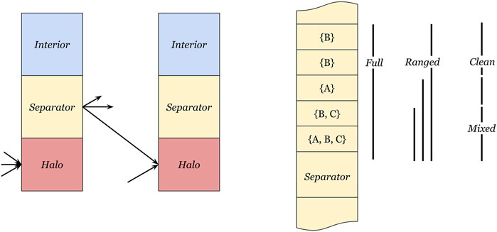
FIGURE 2. Definition of interior, separator, and halo cells. The left side depicts the three cell regions, where the interior region is not communicated, values in the separator region need to be sent to other partitions, and the halo region receives separator values from neighbor partitions. The right side depicts three separator range methods, (full) transmits the entire separator cell range to every neighbor, (ranged) uses the smallest enclosing range for each receiving partition, and (mixed-clean) splits the separator cell range into a mixed part and a clean part.

4.1.1 Full separator communication

The simplest form of separator reordering and outgoing range determination is to declare the full separator region as the outbound region for all neighbors. This has the advantage that the compiler may optimize the internal exchanges to use broadcast operations, having fewer data transmissions on the exchange fabric. The downside is that the whole separator contains values that are not needed for all neighbors. Since the memory is a scarce resource on the IPU, a concern is about the unused values included in these exchanges, as they will also increase the size of the halo region on the receiving partitions.

4.1.2 Ranged separator communication

The ranged separator communication scheme creates one outgoing range from a source tile to each of its destination tiles. Instead of using the whole separator, we can use the smallest range for each destination tile as the outgoing memory region range, which contains all values that must be transferred. As the values cannot be sorted, such that ranges do not overlap, we still transfer the unused values (but fewer) similar to the full separator communication scheme.

4.1.3 Mixed-clean separator communication

To reduce the number of unused values sent, we can split the communication such that up to two ranges are sent to each neighbor partition. The first “mixed” range contains all the values that are required by at least two neighbor partitions, and is transferred in its entirety to all neighbor partitions. The remaining separator values have been sorted by destination partition such that a second “clean” range (containing no unused values) can be sent exclusively to the relevant neighbor.

The advantage of this scheme is that the mixed range can be broadcast from each tile to its neighbor partitions. Furthermore, the clean ranges reduce the number of values transmitted and stored in the halo regions, thus lowering memory usage.

4.2 Specific IPU programming

Porting the existing monodomain simulator to the IPU requires porting two components, a PDE step and an ODE step, each programmed as a Poplar codelet (see Supplementary Section 2.4). The ODE step is independent between the cells; therefore, it can be easily distributed and executed in parallel on all tiles without communication. Each tile goes through all its interior and separator cells and integrates the ODE system for each cell. The required Poplar programming is mostly about deriving a Poplar Vertex class that wraps C functions in the existing monodomain simulator.

The PDE step performs an SpMV (5) involving the voltage values on all the cells. This requires, beforehand, the communication and propagation of halo values between each pair of neighboring tiles. In Poplar, inter-tile communication is described implicitly, as shown in Supplementary Section 2.4. When partitioning the unstructured tetrahedral mesh, we also determine the ranges that need to be communicated from one tile to another. Section 4.1 has described how these ranges are obtained. The globally addressed vector of voltages, V, is required and partitioned into different partitions to be multiplied with the sparse matrix Z, partitioned and stored in the ELLPACK format per tile. Specifically, vector V is decomposed into multiple partitions V_|i,j = V_p with the global index ranging from i to j for the tile with index p.

Here, we recall that each value in vector V is owned by one tile, and the value may be a halo value in one or several tiles. Poplar requires defining the locality of data on the subdomains of tensors. We can do this mapping with, for example, graph.setTileMapping(V.slice(i,j), 123), which maps the range i to j of V to the tile with the identifier of 123. To append halo data into an existing tensor that is already on the tile, we can create a virtual tensor composed of different tensor regions. This virtual tensor will be created through copies and exchanges once the BSP-superstep is launched using this tensor (see Supplementary Section 2.4). Such a virtual tensor can be created by localV = concat(localV, V.slice(m,n)) ∀(m, n) ∈ separatorReceive, where localV is a tensor representing V_p. This simple statement implies the needed tile-to-tile communication, as the ranges (m, n) are owned and computed by other tiles. The compiler automatically generates the exchanges and synchronization steps needed when the PDE compute-vertex using localV is running. On the other hand, localV is not necessarily materialized when the PDE compute-vertex is not running. The memory space can be overwritten by other operations.

Attention must be paid when working with big exchanges of data, as data are duplicated when transferred. Therefore, bigger exchanges can transfer at most half of the per-tile memory in an optimal scenario. An alternative approach is to communicate in smaller chunks to mitigate this problem.

4.3 Performance modeling

On CPUs and GPUs, all hardware optimizations need to be accounted for to determine the expected runtime. Hence, if not performed rigorously, the actual performance can differ dramatically from a predetermined performance model. However, the IPU does not have special hardware optimizations such as caches or instruction pipelining (see Supplementary Section 2.3) and stalling.

Due to the simplicity of the IPU architecture, we can count instructions in any algorithm in the computation phase to create a performance model. In the following, our focus is on the computations involved in the PDE and ODE parts of the monodomain simulator. Using Graphcore’s popc compiler with the -O3 flag, we generated the assembly output for the GC200 platform.

4.3.1 Performance model for the PDE part

On conventional platforms, due to the unstructured computational mesh used, the SpMV operation during each PDE step has to read values that are spread across the main memory. On such systems, due to the random access pattern, the values cannot be fully cached, leading to long runtimes for SpMV.

On the IPU, however, once the sparse matrix and the associated vectors (with halo parts) are partitioned among the tiles, data are only accessed from the local SRAM of each tile. The Poplar code that implements the computation phase of the SpMV is given in Listing 1.

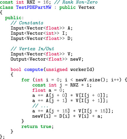
Listing 1. ELLPACK formatted SpMV used for PDE computation.

Counting the instructions of the inner SpMV loop, we estimated for each tetrahedron 107 execution context local cycles and measured a real performance of 106 execution context local cycles. We noticed that of the 107 cycles, 18 cycles are used to store and load spilled registers. Furthermore, the generated code makes use of instruction bundles but does not yet include more specialized instructions available to the GC200, such as headless loops. The one-time start and teardown overhead is 153 instructions.

4.3.2 Performance model for the ODE part

As mentioned in Section 2, the ten Tusscher–Panfilov model (TP06, see [17]) is used for modeling the ionic currents (2–3). An augmented forward Euler scheme is used to explicitly integrate the ODE system (see Section 3.2). By counting the instructions of the TP06 model, we arrive at 1,077 instruction bundles. Adding latencies for the involved math functions (see Supplementary Section 2.2), we get an estimate of 1,401 cycles per tetrahedron (per time step). Adding the loop overhead gives us a total of 1,418 cycles. Our measurements can confirm that the model with 1,415 cycles was actually used. We noticed that 111 instructions, or about 7.9%, were used to handle register spilling. Furthermore, we noticed that the compiler generated 2-element vectorized operations in some places, which is the maximum SIMD operation width for single-precision (32-bit) float values.

5 Math accuracy

The purpose of this section is to rigorously verify the accuracy of some representative mathematical functions when executed on the IPU using single precision. We consider it a very important step before adopting this new processor architecture for numerically solving the monodomain model.

The IPU uses the IEEE754 [28] standard for single-precision floating-point numbers. IEEE754 specifies these as binary32 with one sign bit indicating a positive or negative number, an exponent of 8 bits, and 23 mantissa bits. The general form of a normalized floating-point number can be given as

${\left(m_0.m_1\dots m_p\right)}_2\times {\beta }^e,$

with one significant digit in front of the decimal separator. For the IPU, the base is β = 2, and according to IEEE754, m₀ = 1 is specified.

5.1 Subnormal numbers

The IEEE754 [28] standard formulates an extension of floating-point numbers to subnormal numbers. Subnormal numbers are used to represent numbers smaller than the minimum floating-point number at the loss of accuracy. Subnormal numbers are represented with e_min = 1 − e_max and have m₀ = 0. The numbers they can represent are numbers between zeros and the minimum normalized single-float number. The subnormals are linearly spaced, while normalized floating-point numbers have logarithmic spacing.

The IPU does not support hardware-accelerated subnormals. However, CPUs and GPUs are also not primarily optimized to deal with subnormals. As shown by Fasi et al. [29], V100 and A100 have hardware-accelerated support for subnormals. However, as noted in both Intel and Nvidia developer documentation, subnormals can be an order of magnitude slower than normalized floats.

5.2 Units in the last place

To compare floating-point numbers in one format, such as the IEEE754 single-precision format, we choose the units in the last place (ULP) as a metric rather than the relative error. One ULP is equivalent to

$ulp\left(\beta ,e\right)={\left(0_1.0_2\dots 0_{p-1}{1}_p\right)}_2\times {\beta }^e$

and defined under a constant basis and exponent. One ULP has the scalar distance between representable numbers with bases β and exponent e.

When considering the error, we generally are speaking about the difference from a calculated result $\widehat{y}$ to the mathematically precise and accurate result y:

${\mathrm{e}\mathrm{r}\mathrm{r}\mathrm{o}\mathrm{r}}_{\text{absolute}}=|y-\widehat{y}|.$

We generally cannot precisely represent y in a finite-precision floating-point format, as the true value may always be between two representable numbers. Considering that we are rounding to the nearest number, even with perfect calculation, the error can still be up to 0.5 × ulp (β, e) because we have $\widehat{y}\le y\le \widehat{y}+0.5ulp(\beta ,e)\le \widehat{y}+ulp(\beta ,e)$.

5.3 Experimental setup

We are interested in determining the accuracy of the most important mathematical functions used in our simulator. The functions with one argument that we want to analyze are {exp, expm1, log, sqrt}. The function of interest with two operands is {÷}.

All function operands x_n are represented in the IEEE754 single-precision floating-point format. The results $\widehat{y}$ are like the input operands in single precision. When considering the mathematically accurate result y for a comparison with $\widehat{y}$, we are using double-precision floating-point numbers. However, for $|y-\widehat{y}|$, we are interested in the error represented in ULPs, which gives us a fair estimate of how far we are off in our given representation. Therefore, to get the difference of $y-\widehat{y}$ in ULPs, we need to convert y into the same floating-point format as $\widehat{y}$ with the same base and exponent. This conversion gives us the most accurate result in our chosen representation. We assume the double-precision floating-point result is accurate and precise only with a minimal error, which occurs beyond the representation of single-precision floating-point numbers. Therefore, when converting from double to single precision, we do not introduce an error bigger than 0.5 × ulp (β, e). The final error in ULPs represents how many places in our single-precision representation we are off. For example, if we are able to only represent one place behind the decimal separator with a base and exponent β^e, our accurate mathematical result would be y = 1.3315 × β^e. If we calculated $\widehat{y}=1.5\times {\beta }^e$, while the mathematical result in our representation would be y = 1.3 × β^e, the observed result $\widehat{y}$ is wrong by two ULPs.

For functions with one operand, we can iterate over all single-precision floating-point values as the possible inputs, thus bounded by just 2³² different representable states. However, we are unable to iterate through functions with two operands as the number of possible inputs is not iterable with 2⁶⁴ possible states. Hence, we randomly sample 10 billion different input operand pairs.

5.4 Experiment results

All single-operand math functions {exp, expm1, log, sqrt} and the double-operand function {÷} have been implemented as hardware instructions and specifiable in the assembly. We noticed that subnormal values are rounded off to zero in input, also, if a non-normalized output could be expected. Furthermore, operands that are normalized and produce a subnormal output are rounded off to zero. Both cases are covered in hardware implementation and produce faster results after a single cycle.

All functions showed no more than a 1 × ulp (β, e) error. Errors of one ULP were found randomly distributed throughout the results. Thus, we can say that the single-precision floating-point implementation of the IPU can be considered accurate.

6 Niederer Benchmark

6.1 Running the benchmark

Now, the task is to verify the correctness of our IPU implementation. Ideally, we should choose a well-known problem instance and compare our computational results with real-world measurements. However, cardiac simulations are very complex with multiple parameters and non-trivial geometries. Therefore, the scientific community has agreed to compare multiple codes against each other to create a golden solution that serves as a sensible reference. Niederer et al. [30] formulated an N-version benchmark to compare cardiac electrophysiology simulators independent of the numerical scheme used.

More specifically, the Niederer benchmark uses a box-shaped geometry to represent a 20 × 7 × 3 mm slab of cardiac tissue with fibers aligned along the long (20 mm) axis. A stimulus is applied within a small 1.5 × 1.5 × 1.5 mm cube at a corner of the geometry for a duration of 2 ms and with a stimulation strength of 50000 μA/cm³.

6.2 Benchmark results

As described previously, the Niederer benchmark compares multiple simulation results against each other. As the baseline, we used the existing monodomain code (its CPU version denoted as “OMP” in Figure 3) and executed it on an Intel Xeon CPU with IEEE754-float64 double precision. We compared the IPU implementation of the same cell model to the CPU implementation with more accurate math.

FIGURE 3

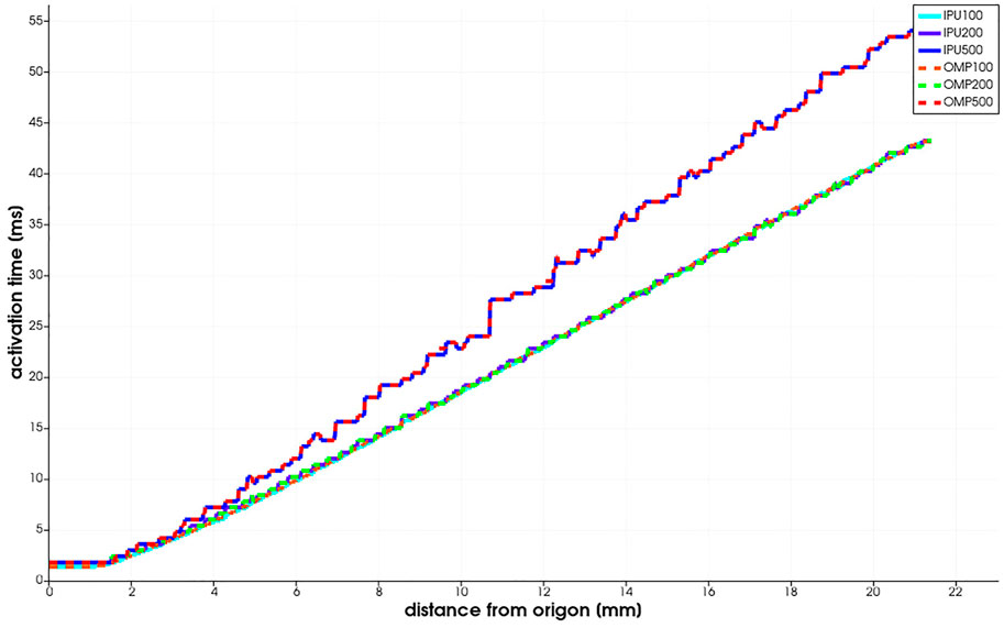
FIGURE 3. Niederer benchmark results reported as the activation time vs. the distance from the stimulus origin.

The benchmark is run for three meshes with 0.5, 0.2, and 0.1 mm resolution. The PDE and ODE time steps are fixed to 0.05 ms. In Figure 3, we observe that the benchmark results computed by the IPU do not diverge significantly from the CPU baseline. When using the same mesh resolution, for example, 0.1 mm, the two implementations produce results that are difficult to distinguish with naked eyes.

In Section 7.4, we will present another comparison of the simulation results between the ported IPU code and an existing GPU implementation. This comparison addresses a realistic heart geometry and unstructured computational meshes.

7 Experiments

7.1 Separator experiments

To determine the effectiveness of the three schemes for reordering and dividing the separator cells on each tile, as discussed in Section 4.1, we use the heart04 mesh (see Section 3.1) as an example. For a given number of IPUs, the unstructured mesh is decomposed by the k-way partitioner of METIS [27] into N sub-meshes, with N equaling the total number of tiles available. For all the experiments, we have always used an imbalance ratio of 3%, while minimizing the adjacency edge-cut, meaning that the number of cells on the largest partition cannot be more than 1.03 times greater than the ideal partition size. This offered us a good trade-off between runtime and partitioning quality. With more workload imbalance, the downsides are twofold: 1) As the IPU uses a bulk synchronous parallel (BSP) programming model, all tiles need to wait until the last tile is finished, leading to poor use of the hardware resources. 2) The maximum problem size which fits on a set of IPUs is reduced because once a single partition becomes too large, the popc compiler fails. Setting a lower work imbalance ratio would reduce the computation time in the PDE and ODE steps, but it might increase the communication volume and, thereby, the time spent on the halo-data exchange phase that occurs before each PDE step.

First, we are interested in the maximum and median memory used on the tiles because the maximum memory requirement per tile indirectly determines how big meshes can fit on a single or multiple IPUs. The second metric of interest is the maximum and median inbound communication volume per tile and the number of unused cells included in the halo regions. To evaluate the effect on a real-world application, we benchmarked the PDE exchange phase and counted the number of cycles used for the exchanges (see details in Section 7.3).

A high-level comparison is shown in Table 1. We can observe that the mixed-clean strategy outperforms the full and ranged strategies. The latter two are on average 2× worse. As expected, the full separator strategy performs consistently worse than the ranged separator strategy. However, the advantage of the mixed-clean strategy may not hold for very small partitions, for example, when the number of IPUs used is very large. This is because as the partitions get smaller, the overlapping ranges in the mixed-clean separator strategy increase, approaching the same level of the full separator strategy. The ranged separator strategy, therefore, may have a small advantage.

TABLE 1

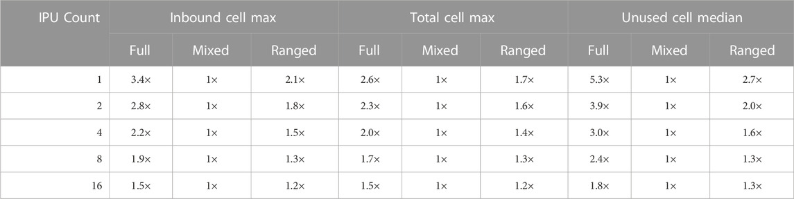
TABLE 1. Partitioning the heart04 mesh using 1 to 16 IPUs under three different exchange strategies. The inbound cells correspond to the halo cells. The total cells are of the biggest partition. Unused cells refer to the cells in the halo region not used by the receiving partition.

When running the real-world benchmarks, such as those to be presented in Section 7.2, we observed a correlation between the number of inbound cells and the exchange time usage. The mixed-clean strategy was thus used when running the IPU-ported monodomain simulator.

7.2 Strong-scaling experiments

We continue with some strong-scaling experiments; that is, the computational mesh is fixed while the number of IPUs increases. For all the IPU numbers tested, we used the heart04 mesh (with 3,031,704 cells) as it is the biggest fitting instance that runs on a single IPU. Figure 4 shows three snapshots from a monodomain simulation using the heart04 mesh. It simulates the propagation of the electrical signal in the heart for 500 ms, with Δt_ODE = 20 μs and Δt_PDE = 5 μs, that is, one ODE step per four PDE steps. In addition to heart04, we also used heart05 (with 7,205,076 cells) for which two IPUs were of the smallest configuration. This mesh has a finer resolution than heart04; thus, a smaller value of Δt_PDE = 4 μs was used, that is, one ODE step per five PDE steps. In addition, we compared the IPU performance with the GPU performance of the existing code [15] using one to eight GPUs in an NVIDIA DGX A100 system. A high-level summary of the comparison is shown in Figure 5, whereas Section 7.4 contains a deep-dive analysis.

FIGURE 4

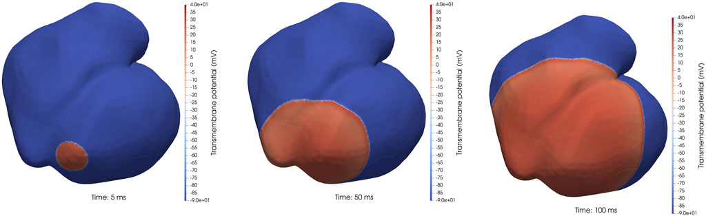
FIGURE 4. Three snapshots of the 3D transmembrane potential field from a realistic monodomain simulation using the heart04 mesh.

FIGURE 5

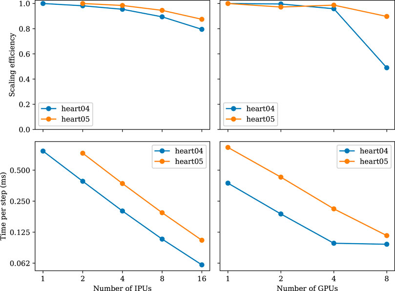
FIGURE 5. Strong-scaling experiments using the meshes of heart04 and heart05. The heart05 mesh is too large for a single IPU.

The k-way partitioner from the METIS software package was used to divide the unstructured meshes, with k equal to the total number of tiles used for each IPU experiment. For the GPU experiments, k is equal to the number of GPUs used. The intra-GPU parallelism utilized the device-level memory accessible for all CUDA threads. All the experiments used a METIS load imbalance constraint of 3%.

Figure 5 shows the results of the strong-scaling experiment. We can observe that both IPU and GPU implementations scale almost linearly. A100 has almost twice the performance and is always matched by twice the number of IPUs. However, when approaching eight GPUs, the scaling efficiency drops. This is not the case for the IPUs, which are able to scale up to 16 IPUs. We were not able to run this experiment on more than 16 IPUs as the popc compilation ran out of memory when trying to compile for 32 IPUs.

When increasing the number of IPUs from 1 to 16 for the heart04 mesh, we observe that the time decreases almost linearly with the added hardware. From the perspective of computation alone, this scaling trend is expected because each tile is responsible for less work. However, due to the increasing number of tiles used, the number of halo cells increases. When using a single IPU for the heart04 mesh, we see a median of 2,058 interior+separator cells per tile and a median of 2,226 halo cells per tile. That is, the halo cells occupy about 51.9% of the total cells per tile. Let us also recall that the values of these halo cells need to be transferred from other tiles before each diffusion step. With more IPUs, the transfer volume increases to about 63.33%, 72.60%, 80.20%, 86.13% of all the cells, for 2, 4, 8, 16 IPUs, respectively. The memory footprints of the halo cells are, thus, steadily increasing.

7.3 Phase breakdown

We used the Graphcore PopVision tools to visualize the inner workings of our IPU-enabled simulator. In order to generate a profile containing runtime and compile information, an environment variable has to be passed during compilation, which will make the Poplar libraries generate profiling information. The profiling information contains static runtime-independent data, such as the memory usage on each tile. Runtime-dependent information is also collected. However, runtime profiling incurs a small performance and memory usage penalty. We are, thus, only interested in the proportions of the execution steps that can be back-adjusted through the non-profiled wall-time usage.

We profiled the four phases of our IPU code, that is, PDE_compute, PDE_exchange, ODE_compute, and ODE_exchange, respectively, based on the computing and exchange phases of the PDE and ODE parts. Table 2 gives a breakdown of the PDE and ODE phases. For example, when using one IPU, the PDE part took about 25.8% of the total execution time, while the data exchange within the PDE steps only took about 1.1%. The computation phase of a PDE step consumes about 22× as much time as the exchange phase. The ODE computation is by far the slowest part, requiring approximately 74.2% of the total execution time. Recall that four PDE steps were executed per ODE step, each ODE step, thus, requires about 11.5× the time of a single PDE step. No communication is required to start the ODE step after the preceding PDE step has finished. Therefore, ODE_exchange is 0. We also noticed that the execution of the ODE step starts without any synchronization.

TABLE 2

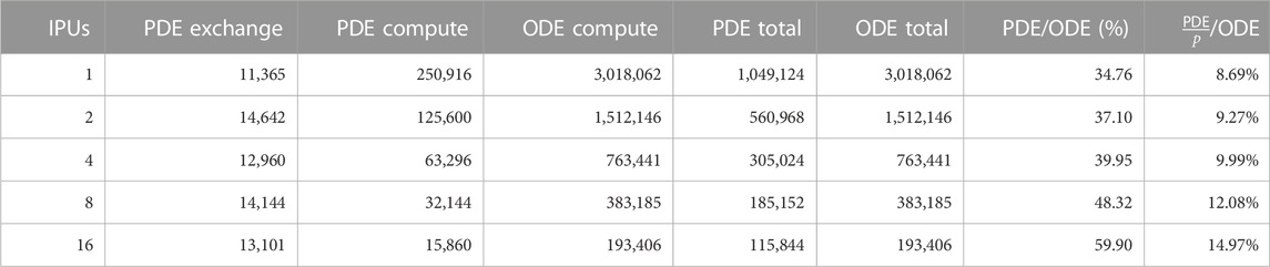
TABLE 2. Breakdown of different algorithmic phases (in number of clock cycles) for the strong-scaling experiments using the heart04 mesh. The PDE per ODE factor p is always four, i.e., four PDE steps per ODE step.

The PDE_compute phase took an average of 238K cycles per tile, where the fastest tile finished after 231K cycles and the slowest after 245K. The standard deviation is 5.2K cycles. However, workload imbalances have no significant impact on the performance because the ODE part can start without requiring global synchronization. ODE_compute took on average 2.8M cycles per tile, with a minimum of 2.7M and a maximum of 2.9M cycles. The standard deviation for ODE_compute is 63.1K cycles.

If we quantify the effectiveness as the percentage of time during which the tiles on average remain non-idle, then the effectiveness is 97% for both the ODE_compute and PDE_compute phases. However, the effectiveness is only 57.4% for the PDE_exchange phase. These numbers are associated with the single-IPU experiment. Using more IPUs will show lower effectiveness, particularly for the PDE_exchange phase, due to a more unbalanced distribution of the halo cells. This problem is currently not properly handled by the mainstream mesh partitioners.

Breaking down the phases of the strong-scaling experiments in Figure 6 shows that the share of communication time (the “PDE exchange” phase) increases. This increasing communication share can be explained by the ladder topology (see Supplementary Figure S2), which increases the latencies linearly with the number of IPUs used.

FIGURE 6

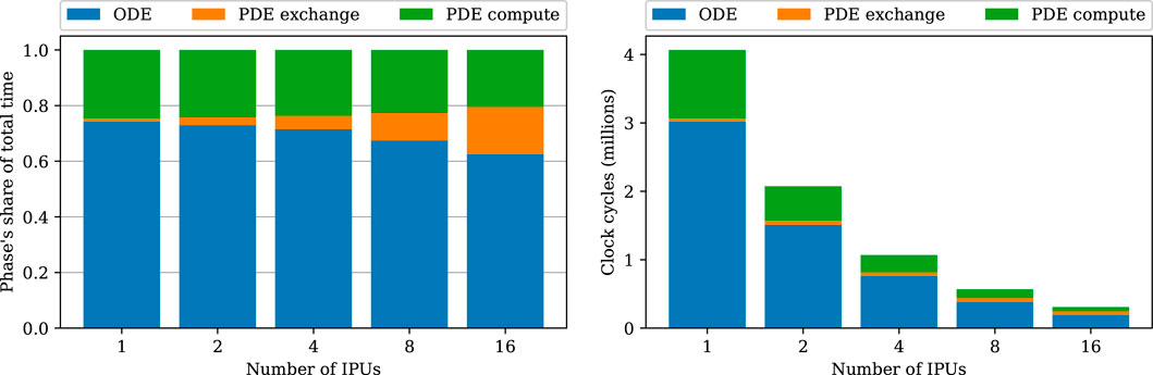
FIGURE 6. Breakdown of the strong-scaling experiments using the heart04 mesh. Blue denotes the total ODE step time composed of only compute, green is the compute phase of the PDE step, and orange denotes the cycles used for PDE exchanges.

7.4 Detailed performance comparison between IPUs and GPUs

Figure 5 has already shown a high-level comparison of the performance between IPUs and GPUs. Now, we want to provide a more detailed performance comparison between two processor architectures, using dissected time measurements of the strong-scaling test with the heart04 mesh.

It can be seen in Table 3 that the GC200 IPUs and A100 GPUs behave very differently for the PDE and ODE parts. It should be noted that the PDE part includes the time spent on halo-data exchanges. The GC200 IPU is considerably more powerful than the A100 GPU for running the SpMVs that constitute the PDE part. We remark that the GPU version of the monodomain simulator is highly optimized as studied in [15]. This can be confirmed by a simple study on the memory traffic. Namely, let us assume perfect data reuse in the L2 cache of the A100 GPU; that is, each value of the input vector ${\vec{v}}_n$ to the SpMV (Eq. 5) is loaded exactly only once from the GPU’s device memory per SpMV. This will produce an idealized lower-bound estimate of the memory traffic on the GPU, which can, in turn, be translated to a minimum bandwidth of 1507.48 GB/s that has been achieved when one A100 GPU is used. Compared with the realistically achievable memory bandwidth of 1774.37 GB/s per A100 GPU, which is measured by the BabelStream micro-benchmark [31], we can conclude that the GPU implementation of the SpMV has achieved at least 85% of the realistically achievable maximum performance. Considering the high level of A100s SpMV performance, it is very impressive that the GC200 IPU beats the A100 GPU in this regard. The explanation lies in the aggregate on-chip SRAM bandwidth of IPU. On the other hand, the GPU performance of the ODE part is much higher than the IPU counterpart, thanks to the GPU’s tremendous floating-point capability. One remark, however, is that GPU implementation can allow a certain level of overlap between the halo-data exchange and the ODE step, which may make the ODE time measurement on the GPU seem shorter than it actually is. This is evident for the ODE time measurement in Table 3 when eight GPUs are used.

TABLE 3

TABLE 3. Performance comparison between GC200 IPUs and A100 GPUs related to a monodomain simulation using the heart04 mesh with 25,000 ODE steps and 100,000 PDE steps.

Last but not least, we have also taken a closer look at the simulated results that are produced by IPU and GPU implementations. Three example snapshots from simulation are shown in Figure 4. Human eyes cannot detect any difference between the two numerical solutions. During the entire simulation that spans 500 ms, the largest maximum difference between the IPU-produced and GPU-produced v values is found to be 0.18 mV. Considering that the simulated v values lie in the range of [−90 mV, 40 mV], this small discrepancy is acceptable.

8 Conclusion

In this work, we have ported an existing simulator of cardiac electrophysiology to Graphcore IPUs. In this process, we investigated the Poplar programming needed and the impact of partitioning and halo-data exchange on SpMV operations that arise from unstructured computational meshes. The speed and accuracy of some special math functions were also rigorously checked on IPUs. These topics are, by no means, constrained to the particular cardiac simulator, but with a good possibility of becoming useful for other computational physics applications.

8.1 Limitations

There are several limitations of the present work. First, the SpMV operations that have been ported to the IPU use the ELLPACK format to store the off-diagonal part of a sparse matrix. This is due to the cell-centered finite volume discretization adopted for the diffusion equation, resulting in the same number of non-zeros per matrix row. In the case of node-centered finite volume discretization or finite element discretization, in general, the number of non-zeros per matrix row will no longer be the same. For example, the standard compressed sparse row format can then be used to store the resulting sparse matrix. This will, however, require a change in the partitioning step, where each row should be weighted by its number of non-zeros. Thus, the sub-meshes can be assigned with different numbers of rows. Such a weighted partitioning scheme actually suits the IPU very well because the computing cost per tile will be strictly proportional to the total number of non-zeros assigned. The GPU counterpart, on the other hand, may need to adopt other storage formats to achieve its full memory bandwidth capacity. This is an active research field illustrated by many recent publications such as [32].

Second, still with respect to the partitioning step, the present work has another limitation related to using multiple IPUs. Our current partitioning strategy is single-layered, that is, an unstructured mesh is decomposed into as many pieces as the total number of IPUs available on multiple IPUs. No effort is made to limit the halo-data exchanges that span between IPUs. As shown in Supplementary Figure S2 in Supplementary Section 2.1, the communication speed between IPUs is heterogeneous and much lower than the intra-IPU communication speed between the tiles. An idea for improvement is to introduce a hierarchical partitioning scheme, where a first-layer partitioning concerns only the division between the IPUs, whereas a second-layer partitioning divides further for the tiles within each IPU. Moreover, the partitioning on both layers should attempt to evenly distribute the halo cells. Otherwise, tiles over-burdened with halo cells will quickly become the bottlenecks.

Third, we have only considered explicit time integration for the diffusion equation. The upside is that the PDE solver only needs SpMVs, but the downside is the severe stability restriction on the size of Δt_PDE. Implicit time integration is good to have with respect to numerical stability but will give rise to linear systems that need to be solved. Here, we remark that SpMVs constitute one of the building blocks of any iterative linear solver.

8.2 Lessons learned

The design of algorithms must be reconsidered for massively tiled processors. While the HPC community already has ample experience in using technologies like distributed memory and BSP, their use in the IPU has not been explored equally well. Most of the current projects and their underlying design considerations are not adjusted to the trade-offs of this new class of accelerators. New ways to think of communication and load balance are necessary.

Furthermore, Poplar programming requires us to implicitly define communication at compile time. This makes it impossible to have predefined kernels such as those commonly found on CPUs and GPUs. One could argue that the compilation of regular-mesh kernels for IPUs only needs to happen once for all inputs. However, compiling irregular meshes is required for every single communication scenario unless a regular representation can be found. This unavoidable compilation requires us to be aware of the expensive compilation time. We also found that the compilation time and mesh preprocessing time substantially increase with multiple IPU devices.

The current IPU architecture also has clear limitations. These include the support of only single-precision computing and limited SRAM resource per tile. Instead of waiting for Graphcore to develop new IPUs capable of double-precision computing, a possible strategy can be used to identify the most accuracy-critical parts of a computation and emulate double-precision operations by software for these parts, whereas the remaining parts use single precision. Better partitioning algorithms, which adopt a hierarchical approach and are aware of the heterogeneity in the communication network, will also be useful for optimizing the usage of the limited SRAM per tile. On the other hand, we should not forget about one particular advantage of AI processors such as IPUs. That is, these processors are already good at running machine-learning workloads. Thus, if “conventional” scientific computing tasks can be efficiently ported to AI processors, the distance to converged AI and HPC is short.

In future work, we will investigate further optimizations of halo-data exchanges both on and between the IPUs (with the help of better partitioning strategies) and extend our work to other more general unstructured-mesh computations.

Data availability statement

The raw data supporting the conclusion of this article will be made available by the authors, without undue reservation.

Author contributions

All the authors contributed to the conceptualization of the work. LB designed and implemented the IPU code, performed the related experiments, and collected the measurements. The original GPU version of the Lynx code was designed and implemented by JL, with the ODE part added by KGH. KGH performed all the GPU experiments. All the authors participated in the discussions and analyses of the experimental results. All the authors contributed to the writing of the manuscript.

Funding

The work of the second author was partially supported by the European High-Performance Computing Joint Undertaking under grant agreement No. 955495 and the Research Council of Norway under contract 329032. The work of the third and fourth authors was partially supported by the European High-Performance Computing Joint Undertaking under grant agreement No. 956213 and the Research Council of Norway under contracts 303404 and 329017. The research presented in this paper benefited from the Experimental Infrastructure for the Exploration of Exascale Computing (eX3), which was financially supported by the Research Council of Norway under contract 270053.

Acknowledgments

Julie J. Uv segmented the surface files that were used to generate fiber directions for the bi-ventricular meshes. James D. Trotter generated the meshes with fiber directions.

Conflict of interest

The authors declare that the research was conducted in the absence of any commercial or financial relationships that could be construed as a potential conflict of interest.

Publisher’s note

All claims expressed in this article are solely those of the authors and do not necessarily represent those of their affiliated organizations, or those of the publisher, the editors, and the reviewers. Any product that may be evaluated in this article, or claim that may be made by its manufacturer, is not guaranteed or endorsed by the publisher.

Supplementary material

The Supplementary Material for this article can be found online at: https://www.frontiersin.org/articles/10.3389/fphy.2023.979699/full#supplementary-material

References

1. Bern M, Plassmann P. Chapter 6–mesh generation. In: JR Sack, and J Urrutia, editors. Handbook of computational geometry. North-Holland (2000). p. 291–332. doi:10.1016/B978-044482537-7/50007-3

CrossRef Full Text | Google Scholar

2. Unat D, Dubey A, Hoefler T, Shalf J, Abraham M, Bianco M, et al. Trends in data locality abstractions for HPC systems. IEEE Trans Parallel Distributed Syst (2017) 28:3007–20. doi:10.1109/TPDS.2017.2703149

CrossRef Full Text | Google Scholar

3. Buluç A, Meyerhenke H, Safro I, Sanders P, Schulz C. Recent advances in graph partitioning. Algorithm engineering: Selected Results and surveys (springer). Lecture Notes Comp Sci (2016) 9220:117–58. doi:10.1007/978-3-319-49487-6_4

CrossRef Full Text | Google Scholar

4.cerebras. The future of AI is here (2022). Available at: https://cerebras.net/chip/ (Accessed June 25, 2022).

Google Scholar

5.GRAPHCORE. Designed for AI–intelligence processing unit (2021). Available at: https://www.graphcore.ai/products/ipu (Accessed June 25, 2022).

Google Scholar

6.Message Passing Interface Forum. Mpi: A message-passing interface standard version 4.0 (2021).

Google Scholar

7. Mohan LRM, Marshall A, Maddrell-Mander S, O’Hanlon D, Petridis K, Rademacker J, et al. Studying the potential of Graphcore IPUs for applications in particle physics (2020). arXiv preprint arXiv:2008.09210.

Google Scholar

8. Ortiz J, Pupilli M, Leutenegger S, Davison AJ. Bundle adjustment on a graph processor. In: Proceeding of the 2020 IEEE/CVF Conference on Computer Vision and Pattern Recognition (CVPR); June 2020; Seattle, WA, USA. IEEE Computer Society (2020). p. 2413–22. doi:10.1109/CVPR42600.2020.00249

CrossRef Full Text | Google Scholar

9. Burchard L, Moe J, Schroeder DT, Pogorelov K, Langguth J. iPUG: Accelerating breadth-first graph traversals using manycore Graphcore IPUs. In: International conference on high performance computing. Springer (2021). p. 291–309.

CrossRef Full Text | Google Scholar

10. Burchard L, Cai X, Langguth J. iPUG for multiple Graphcore IPUs: Optimizing performance and scalability of parallel breadth-first search. In: Proceeding of the 2021 IEEE 28th International Conference on High Performance Computing, Data, and Analytics (HiPC); December 2021; Bengaluru, India. IEEE (2021). p. 162–71. doi:10.1109/HiPC53243.2021.00030

CrossRef Full Text | Google Scholar

11. Rocki K, Van Essendelft D, Sharapov I, Schreiber R, Morrison M, Kibardin V, et al. Fast stencil-code computation on a wafer-scale processor. In: Proceedings of the International Conference for High Performance Computing, Networking, Storage and Analysis; November 2020. IEEE Press (2020). p. 1–14. SC ’20.

CrossRef Full Text | Google Scholar

12. Jacquelin M, Araya-Polo M, Meng J. Massively scalable stencil algorithm (2022). arxiv.2204.03775. doi:10.48550/ARXIV.2204.03775

CrossRef Full Text | Google Scholar

13. Louw TR, McIntosh-Smith SN. Using the Graphcore IPU for traditional HPC applications. In: Proceedings of the 3rd Workshop on Accelerated Machine Learning: Co-located with the HiPEAC 2021 Conference; 18-01-2021. Budapest, Hungary: AccML (2021).

Google Scholar

14. Håpnes S. Solving partial differential equations by the finite difference method on a specialized processor. Master’s thesis. Oslo, Norway: University of Oslo (2021). Available at: http://urn.nb.no/URN:NBN:no-92505 (Accessed June 25, 2022).

Google Scholar

15. Hustad KG. Solving the monodomain model efficiently on GPUs. Master’s thesis. Oslo, Norway: University of Oslo (2019). Available at: http://urn.nb.no/URN:NBN:no-74080 (Accessed June 25, 2022).

Google Scholar

16. Clayton RH, Bernus O, Cherry EM, Dierckx H, Fenton F, Mirabella L, et al. Models of cardiac tissue electrophysiology: Progress, challenges and open questions. Prog Biophys Mol Biol (2011) 104:22–48. doi:10.1016/j.pbiomolbio.2010.05.008

PubMed Abstract | CrossRef Full Text | Google Scholar

17. ten Tusscher KH, Panfilov AV. Cell model for efficient simulation of wave propagation in human ventricular tissue under normal and pathological conditions. Phys Med Biol (2006) 51:6141–56. doi:10.1088/0031-9155/51/23/014

PubMed Abstract | CrossRef Full Text | Google Scholar

18.KHWJ ten Tusscher. Source code second version human ventricular cell model (2021). [Dataset]. Available at: http://www-binf.bio.uu.nl/khwjtuss/SourceCodes/HVM2/ (Accessed June 25, 2022).

Google Scholar

19. Martinez-Navarro H, Rodriguez B, Bueno-Orovio A, Minchole A. Repository for modelling acute myocardial ischemia: Simulation scripts and torso-heart mesh (2019). [Dataset]. Available at: https://ora.ox.ac.uk/objects/uuid:951b086c-c4ba-41ef-b967-c2106d87ee06 (Accessed June 25, 2022).

Google Scholar

20. Bayer JD, Blake RC, Plank G, Trayanova NA. A novel rule-based algorithm for assigning myocardial fiber orientation to computational heart models. Ann Biomed Eng (2012) 40:2243–54. doi:10.1007/s10439-012-0593-5

PubMed Abstract | CrossRef Full Text | Google Scholar

21. Marsh ME, Ziaratgahi ST, Spiteri RJ. The secrets to the success of the Rush–Larsen method and its generalizations. IEEE Trans Biomed Eng (2012) 59:2506–15. doi:10.1109/TBME.2012.2205575

PubMed Abstract | CrossRef Full Text | Google Scholar

22. Mirin AA, Richards DF, Glosli JN, Draeger EW, Chan B, Fattebert J, et al. Toward real-time modeling of human heart ventricles at cellular resolution: Simulation of drug-induced arrhythmias. In: SC’12: Proceedings of the International Conference on High Performance Computing, Networking, Storage and Analysis; November 2012; Salt Lake City, UT, USA. IEEE (2012). doi:10.1109/SC.2012.108

CrossRef Full Text | Google Scholar

23. Rush S, Larsen H. A practical algorithm for solving dynamic membrane equations. IEEE Trans Biomed Eng (1978) BME-25(4):389–92. doi:10.1109/tbme.1978.326270

PubMed Abstract | CrossRef Full Text | Google Scholar

24. Langguth J, Sourouri M, Lines GT, Baden SB, Cai X. Scalable heterogeneous CPU-GPU computations for unstructured tetrahedral meshes. IEEE Micro (2015) 35:6–15. doi:10.1109/mm.2015.70

CrossRef Full Text | Google Scholar

25. Langguth J, Wu N, Chai J, Cai X. Parallel performance modeling of irregular applications in cell-centered finite volume methods over unstructured tetrahedral meshes. J Parallel Distributed Comput (2015) 76:120–31. doi:10.1016/j.jpdc.2014.10.005

CrossRef Full Text | Google Scholar

26. Grimes RG, Kincaid DR, Young DM. ITPACK 2.0 user’s guide. Austin, TX: Center for Numerical Analysis, University of Texas (1979).

Google Scholar

27. Karypis G, Kumar V. A fast and high quality multilevel scheme for partitioning irregular graphs. SIAM J Scientific Comput (1998) 20:359–92. doi:10.1137/S1064827595287997

CrossRef Full Text | Google Scholar

28.IEEE. IEEE standard for floating-point arithmetic. IEEE Std 754-2008 (2008). p. 1–70. doi:10.1109/IEEESTD.2008.4610935

CrossRef Full Text | Google Scholar

29. Fasi M, Higham NJ, Mikaitis M, Pranesh S. Numerical behavior of NVIDIA tensor cores. PeerJ Comp Sci (2021) 7:e330. doi:10.7717/peerj-cs.330

CrossRef Full Text | Google Scholar

30. Niederer SA, Kerfoot E, Benson AP, Bernabeu MO, Bernus O, Bradley C, et al. Verification of cardiac tissue electrophysiology simulators using an n-version benchmark. Philos Trans R Soc A: Math Phys Eng Sci (2011) 369:4331–51. doi:10.1098/rsta.2011.0139

CrossRef Full Text | Google Scholar

31.BabelStream. BabelStream (2022). [Dataset]. Available at: https://github.com/UoB-HPC/BabelStream (Accessed June 25, 2022).

Google Scholar

32. Mohammed T, Albeshri A, Katib I, Mehmood R. Diesel: A novel deep learning-based tool for SpMV computations and solving sparse linear equation systems. The J Supercomputing (2021) 77:6313–55. doi:10.1007/s11227-020-03489-3

CrossRef Full Text | Google Scholar

33. Jia Z, Tillman B, Maggioni M, Scarpazza DP. Dissecting the Graphcore IPU architecture via microbenchmarking (2019). arXiv preprint arXiv:1912.03413.

Google Scholar

34. Valiant LG. A bridging model for parallel computation. Commun ACM (1990) 33:103–11. doi:10.1145/79173.79181

CrossRef Full Text | Google Scholar

35. Abadi M, Isard M, Murray DG. A computational model for TensorFlow: An introduction. In: Proceedings of the 1st ACM SIGPLAN International Workshop on Machine Learning and Programming Languages; June 2017. Barcelona, Spain: ACM (2017). p. 1–7.

CrossRef Full Text | Google Scholar