Symbol error rate minimization using deep learning approaches for short-reach optical communication networks

1 Introduction

Over the last few years, there has been significant development in optical transmission systems to meet the increasing demands of the telecommunications sector. These advancements stem from the numerous advantages of optical fiber, which include swifter transmission, reduced signal loss (attenuation), smaller physical dimensions, heightened resistance to electromagnetic interference, and greater capacity for data transmission. Presently, there is substantial interest in short-distance communication systems within both industry and academia. The term “short-reach” pertains to communication setups with transmission distances under 100 km, which are cost-sensitive due to their widespread deployment [1, 2]. Short-reach optical communication encounters more intricate challenges owing to factors like the advent of 5G technology, the envisioned developments beyond 5G (referred to as 6G), the utilization of edge-distributed cloud computing networks, extensive machine-to-machine communications, communication within or between data centers, and mobile front-haul setups [1, 3, 4]. For the sake of discussion, short-reach optical networks can be classified into five categories based on their transmission distance and function: inter-data center networks, intra-data center networks, optical access networks, indoor and in-building optical wireless communications, and mobile front-haul communications. Communication requirements are becoming progressively rigorous, and the intricacy of short-reach optical networks grows significantly across these various types. To tackle these challenges, there is a growing proposal and extensive study of incorporating artificial intelligence (AI) in short-reach optical systems. AI emulates biological processes like learning, self-correction, and extrapolation, enabling computers to manage complex scenarios. In recent decades, the application of AI to enhance the performance of optical networks and systems has emerged as a prominent area of research, encompassing network management and transmission. Machine learning (ML), a subset of AI, empowers an agent to enhance its future task execution by learning from past experiences.

ML techniques have garnered significant attention within the realm of short-reach optical communication systems due to their aptitude for problem-solving, decision-making, and pattern recognition. Their application is widespread in various aspects of short-reach optical systems, encompassing tasks such as optical performance monitoring (OPM), signal processing, modulation format identification (MFI), and indoor optical wireless systems.

In the context of short-reach optical systems that use compact and cost-effective components, such as those utilizing direct detection receivers, achieving desired data rates in a cost-efficient manner requires innovative signaling and digital signal processing (DSP) techniques. As an alternative to conventional DSP methods, ML algorithms are emerging as effective solutions for addressing nonlinear challenges. Neural networks can also play a role in optimizing transmitter or receiver DSP functions [5]. In short-reach optical networks based on intensity modulation/direct detection (IM/DD) techniques, which are known for their cost-effectiveness, photodiodes are used to detect nonlinear signals. The presence of dispersion can lead to significant impairments, notably intersymbol interference (ISI). To combat these challenges and enhance system performance, ML techniques are gaining traction as viable alternatives to traditional DSP approaches [1, 6]. These ML-based techniques, such as equalization, autoencoders (AEs), digital pre-distortion, and soft-demapping, have been employed in various ways, encompassing compensation for both linear and nonlinear distortions (NLDs).

To tackle the challenge of compensating for both linear and nonlinear distortions in optical networks, advanced techniques such as maximum likelihood sequence estimation (MLSE) and equalizers based on ML algorithms are under exploration [7]. Among these approaches, ML-based methods, particularly those leveraging neural networks, are gaining recognition for their effectiveness in equalization tasks. Neural networks are being employed either to assist other signal processing stages or directly as comprehensive equalizers. These studies highlight that neural networks outperform traditional equalizers, positioning them as a sought-after technology with significant value in short-reach applications [8]. Various architectural designs have been proposed for this purpose, including feedforward neural networks (FFNNs) [9–11], reservoir computing (RC) [12–18], and recurrent neural networks (RNNs) [19, 20]. These architectures can be effectively utilized for both linear and nonlinear equalization tasks.

Similarly, there exist signal processing methods such as autoencoders [21–24] that facilitate the development of end-to-end processes where the transmitter, channel, and receiver are jointly optimized. This idea was first introduced for wireless communication [25–27] and later quickly utilized for optical fiber communications [6, 21]. Autoencoders comprise three key components: the encoder, code, and decoder. The encoder reduces input dimensionality, and the decoder restores the reduced code dimension. This process retains essential features of the input data after dimensionality reduction, leading to reduced transmission rates and enhanced communication reliability [21]. A proposal involving fully connected neural networks and a bidirectional LSTM (BiLSTM) model for the channel introduces an autoencoder for intensity modulation/direct detection (IM/DD) systems [22]. This auto-encoder capitalizes on optical signal characteristics in the time domain and incorporates various system factors like nonlinearity, attenuation, dispersion, and optical-to-electrical square-law conversion. The primary goal of the auto-encoder is to minimize the dimensions of the input signal, thereby enhancing system reliability and reducing transmission rates while preserving essential features.

When addressing impairments such as linear and nonlinear distortions in power amplifiers, a widely used technique is digital pre-distortion (DPD), which commonly employs Volterra-based algorithms involving intricate direct and indirect learning architectures [28]. To offer a lower-complexity alternative to Volterra-based algorithms, an approach using an extreme learning machine (ELM) for DPD has been proposed. This method enables rapid estimation and compensation of transfer functions, including those of Mach–Zehnder modulators (MZMs) [29]. In the realm of DPD, an ML-based approach utilizing FFNNs has been recommended to enhance the power efficiency of radio-over-fiber (RoF) links in analog optical front-haul applications [28].

For achieving high spectral efficiency and speed in optical communication networks, technologies like soft decision forward error correction (FEC) and higher-order quadrature amplitude modulation (QAM) have been studied. When dealing with nonlinear equalization (NLE) and soft decision de-mapping in Volterra-based equalization, complexity can be a challenge. An alternative approach employs a soft neural network (NN) based method known as soft deep neural network (SDNN) architecture. This approach is explored for its ability to address the temporal dynamic behavior of sequences of time, providing an effective solution to nonlinearities [30]. Likewise, a soft de-mapper based on bidirectional RNN techniques has been suggested [31] in the context of improving performance compared to a soft de-mapper based on artificial neural networks (ANNs) [30, 32]. This approach capitalizes on the ability of bidirectional RNNs to represent infinite impulse responses and nonlinearities, thereby effectively capturing the temporal dynamic behavior of sequences of time.

This study focuses on employing deep learning models to reduce symbol error rates in short-distance optical communication configurations. We accurately simulate various channel impairments like nonlinearity, CD, and attenuation. Initially, we tackle the task of modeling a nonlinear channel. Subsequently, we use autoencoders, a type of deep learning model, to aid communication over nonlinear channels. Additionally, we examine how integrating a nonlinear channel into an autoencoder affects the received constellation as the length of the optical fiber increases. Another aspect of our research involves implementing a receiver based on deep neural networks, which operate in a channel influenced by chromatic dispersion. By gradually increasing the optical length, we analyze its influence on the received constellation and, consequently, the symbol error rate. Lastly, we introduce the split-step Fourier method (SSFM) to simulate the combined impacts of nonlinearities, chromatic dispersion, and attenuation in the optical channel. This simulation is achieved through a neural network-based receiver approach. The remainder of this paper is structured as follows: in Section 2, we describe the basic concepts of deep learning and autoencoders. The proposed architecture of the autoencoder is presented in Section 3. Section 4 explains the simulation scenarios based on different channel impairments along with their effect on model performance. In Section 5, the split-step Fourier method and its simulation parameters are discussed. Finally, the conclusion and future work directions are given in Section 6.

2 Background

This section introduces the DNNs [33, 34] and AEs.

2.1 Fully connected deep neural networks

A feedforward model, such as a N-layer fully connected DNN, maps an input vector v₀ to an output vector v_N = f_DNN(v₀) through repetitive steps of the form is given by

$v_n={\alpha }_n\left({\mathbf{W}}_n{v}_{n-1}+{\mathbf{b}}_n\right),n=\mathrm{1,2},\dots .N,(1)$

where v_n−1 is the output of (n − 1)th layer, v_n is the output of nth layer, W_n is the weight matrix, b_n is the bias vector of nth layer, and α_n is the activation layer [21]. The parameters W_n and b_n of the layer are represented by

${\theta }_n=\left\{{\mathbf{W}}_n,{\mathbf{b}}_n\right\}.(2)$

The network is capable of approximating nonlinear functions through the use of the activation function α_n, which establishes nonlinear relationships between the layers. The rectified linear unit (ReLU) is a frequently used activation function in modern ANNs. It acts separately on each of its input vector elements by maintaining the positive values and equating negative to zero [35], i.e., z = α_Relu(k) with

$z_i=max\left(0,k_i\right),(3)$

where z and k are vectors whose ith elements are represented by z_i and k_i, respectively. The ReLU function has a continuous gradient when compared to other well-known activation functions like the hyperbolic tangent and sigmoid, which makes training computationally less expensive and prevents the effect of vanishing gradients. This impact happens for activation functions with asymptotic behavior because the gradient can shrink and slow the learning algorithm’s convergence.

The softmax activation function is frequently used in the last (decision) layer of an ANN, and the elements z_i of the output z = softmax k) are provided by

$z_i=\frac{exp\left(k_i\right)}{{\sum }_{j}exp\left(k_j\right)}.(4)$

By labeling the training data, the neural network training may be performed under supervision. This establishes a pairing between the intended output vector ${\widehat{v}}_N$ and input vector v₀. As a result, the training goal is to minimize the cost function $\mathcal{C}({\mathbf{W}}_n,{\mathbf{b}}_n)$ as a function of the weight matrix, W_n, and bias vector, b_n, of all N layers. The cost function over the set of training inputs M between the DNN output, v_N, and intended output,${\widehat{v}}_N$, is given by

$\mathcal{C}\left({\mathbf{W}}_n,{\mathbf{b}}_n\right)=\frac{1}{|M|}{\displaystyle \sum _{i=1}^M}L\left(v_0,{\widehat{v}}_N\right).(5)$

In Eq. 5, L (z, k) represents the loss function and |M| is the training example number. Cross-entropy is the loss function that we used in this work, represented as

$L\left(k,z\right)=-{\displaystyle \sum _i}{k}_i\log z_i.(6)$

In modern deep learning, error backpropagation allows for efficient computation of the gradient [33]. Adam optimizer, a cutting-edge algorithm with improved convergence, dynamically changes the learning rate η [36]. In this work, training process optimization is carried out using the Adam algorithm, and PyTorch and Keras [37] were used to create all of the numerical results.

2.2 Basics of autoencoder

An AE is a concept in which data are first encoded into a compressed form and subsequently decoded to revert it to its original shape. This technique, employed in unsupervised learning, involves acquiring a condensed representation of input data through the utilization of an NN. This acquired representation can then be effectively applied to tasks such as reducing noise, compressing data, or extracting features. The autoencoder is composed of three primary components: the encoder section, a code, and the decoder section. The encoder element takes the input data and compresses it into a lower-dimensional form referred to as the encoded data or code. This compressed representation is usually presented as a vector of numerical values, serving as a compact summary of the input data. This implies that the encoder’s function is to compress the data. Within the encoder, one or more hidden layers exist that apply nonlinear transformations to the data, generating the encoded version. The structure of an autoencoder is depicted in Figure 1. Subsequently, the code is input into the decoder phase, which effectively reconstructs the initial data, namely, the input data, from the dimensionally reduced code. This decoder is comprised of one or more concealed layers that undertake the task of transforming the condensed representation back into the original data form. The objective of the decoder’s output is to closely mirror the input data. The primary aim is to restore the original data with minimal loss of information from the compressed representation.

Figure 1

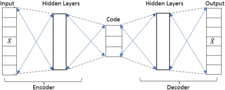
Figure 1. Structure of an autoencoder.

A loss function is employed to minimize disparities between the input and reconstructed data, often using metrics like mean squared error, during the training process of the AE. The weights of both the encoder and decoder are updated through the utilization of backpropagation and optimization algorithms like stochastic gradient descent. Figure 2 illustrates the sequential progression of the autoencoder. Beginning with the input data, the autoencoder undertakes the task of learning how to extract the most pivotal features and subsequently encapsulate them in a streamlined manner. This is achieved by implementing a bottleneck layer within the network’s core, housing fewer neurons in comparison to the input and output layers. Through this method of data compression, the autoencoder gains the ability to understand the process of discarding irrelevant information while concentrating on the most significant and critical features. Upon the successful training of the autoencoder, the code generated by the encoder can be harnessed for various purposes, such as data compression or feature extraction. For instance, if the autoencoder has been trained on images, the compact representation of the image, i.e., the code produced by the encoder, can be applied for tasks like image retrieval or classification.

Figure 2

Figure 2. Flow process of an AE.

Autoencoders possess the remarkable capacity to acquire valuable data representations devoid of the necessity for labeled data, which stands out as a significant advantage. This attribute renders them particularly advantageous for tasks where acquiring labeled data is resource-intensive or challenging. Moreover, autoencoders exhibit proficiency in handling high-dimensional data, a domain often fraught with challenges for other categories of machine learning algorithms. Nonetheless, grappling with overfitting remains one of the principal hurdles associated with autoencoders. This occurs when the autoencoder predominantly learns the intricacies of the training data features rather than cultivating valuable, generalizable features suitable for new data instances. To counteract the menace of overfitting, regularization approaches such as dropout techniques and weight decay methods can be harnessed. These strategies serve to maintain the autoencoder’s focus on salient and broadly applicable features, curbing the inclination toward excessive adaptation to training data specifics.

3 Proposed end-to-end communication system

We put into practice a fiber optic communication system and transmission chain, including the transmitter, receiver, and channel, as a full end-to-end ANN, as suggested in [26, 27]. The above-stated concept has been extended to the interpretation of communication system components, consisting of the transmitting part, channel, and receiving part. Figure 3 shows the basic components of the communication system, which consists of the transmitter, channel, and receiver.

Figure 3

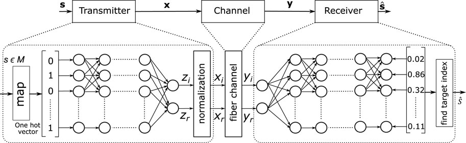
Figure 3. Illustration of the proposed autoencoder.

The proposed autoencoder structure is shown in Figure 3. A message s is sent, which is chosen from a pool of M possible messages {1, 2, … , M}≜M. For every message, log₂M bits are represented. In accordance with (30), first the messages are converted into “one hot encoded” vectors of dimension M, where 1 is the sth element and the other remaining elements are represented by 0. These vectors are fed as an input to transmitter NN, which contains numerous layers of densely connected neurons. Every neuron receives inputs from the layer before it and produces an output based on z_out = f (w^Tz_in + b), where w represents a vector of weights, b ∈ R denotes a bias, and f (⋅) is the activation function, which is assumed to be linear in this case.

The transmitter’s two outputs z_i and z_r are used as inputs to the channel. To satisfy the constraint of average power, the NN is normalized by the use of M different training inputs. The input of the channel, denoted as x, is selected randomly by a constellation consisting of M points with a second moment E [|x|²] = P_in, where P_in is equivalent to the input power. After that, the normalized output is transmitted through the channel, and y output is produced. The channel output y consisting of real y_r element and imaginary y_i element are fed to a receiver NN as an input. The receiver NN outputs a probability distribution f_y (s′) in [0,1], s′ ∈ M over all possible transmitted messages represented by set M. The output is normalized to ensure that the sum of all probabilities should be equal to 1. The estimated transmitted message $\widehat{s}$ is then obtained by selecting the message with the highest probability from the output distribution, given by s = argmax_s′, f_y (s′) [38].

4 Simulation scenarios and results

In this section, different channel impairments have been modeled and their effects on the communication system have been explained.

4.1 Nonlinearity based channel

First, we consider the effects of nonlinear phase noise in single-mode optic fiber models. The nonlinear Schrödinger equation (NLSE) is used for modeling the propagation of signals in an optical fiber employing distributed amplification as follows [39]:

$\frac{\partial k\left(d,t\right)}{\partial d}=i\gamma \Vert k\left(d,t\right){\Vert }^2-i\frac{{\beta }_2}{2}\frac{{\partial }^{2}x\left(d,t\right)}{\partial d^2}-p\left(d,t\right).(7)$

Here, k (d, t) is the signal, which is transmitted, t is the time coordinate, and d is the distance coordinate; the nonlinearity parameter is represented by γ, β₂ is the group velocity dispersion (GVD) coefficient, and the Gaussian noise is represented by p (d, t). The right side of the equation has two terms. The equation’s first term shows the Kerr effect, which induces a shift in the phase that is proportional to the signal’s power and leads to a substantial distortion in optical fiber systems. The second term shows dispersion. As the channel likelihood function in [Eq. 7] is unknown, a simple dispersionless channel is considered by ignoring β₂ in [Eq. 7]. The equation of the model based on recursion is given as follows [40]:

$k_{i+1}=k_i{e}^{j{L}_o\gamma |k{|}^2/S}+p_{i+1},0\le i\le S.(8)$

Here, k₀ = k is the input to the channel consisting of complex values, r = k_S is the output of the channel, p_i+1 ∼ CN(0, P_N/S), fiber link length is represented by L_o, γ is the nonlinearity parameter, and P_N is the noise power. Ideal distributed amplification is assumed by the model and S → ∞.

4.2 Learned constellations

To obtain numerical results, the fiber model in [Eq. 8] is assumed to have an optical fiber length of L_o = 100 km, a nonlinearity coefficient of γ = 1.27, and a noise power of P_N = −21.3 dBm. The model is iterated S = 50 times for simulation, providing a good approximation of the true asymptotic channel PDF [41].

Using PyTorch’s random number generator, the dataset gets generated inside the network on the fly. The training dataset size is 1.10⁴. The number of Epochs = 120, and the batch size is varied during the training. The size of the validation dataset is 1.10⁵. The cross-entropy loss function and Adam optimizer [36] in PyTorch are used for training the AE separately for various values of P_in. The AE structure parameters for M = 16 are summarized in Table 1.

Table 1

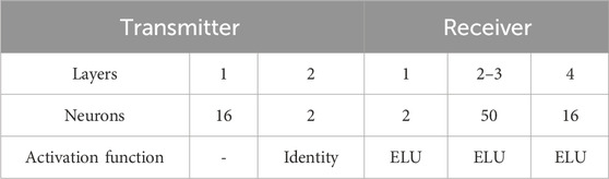
Table 1. Autoencoder parameters for M = 16.

In Figure 4, the 16-point constellation that has been learned under different P_in for nonlinearity-based fiber optic channels is shown. The points in the learned constellation are equally spaced and pentagonal-shaped at −11 dBm, as shown in Figure 4A. In highly nonlinear regimes, the constellations appear to be random. The constellation points with high energy have varying radii. As a result, after propagation through the nonlinear fiber channel, these points do not overlap with other points. Additionally, the farther the point is from others, the larger its radius.

Figure 4

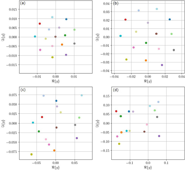
Figure 4. Nonlinear fiber channel 16-point learned constellations for different P_in values. (A) P_in = −11 dBm. (B) P_in = −1 dBm. (C) P_in = 6 dBm. (D) P_in = 12 dBm.

4.3 Effect of the nonlinear channel on fiber length

In a nonlinear channel, when the length of the optical fiber increases, the nonlinearity of the fiber increases as well, leading to signal quality degradation, which can limit the achievable transmission distance and data rate. For obtaining different numerical results, consider the optic fiber model in [Eq. 8] with a nonlinearity coefficient of γ = 1.27, noise power of P_N = −21.3 dBm, and input power of P_in = 2 dBm. Table 1 shows the autoencoder parameters used for different lengths. For training the model, the number of Epochs = 120, and the batch size is varied during the training. In the initial iteration, the batch size is kept small to obtain a working solution. The size of the batch increases as the training nears completion. If the size of the batch is kept small, there will be no misclassifications, and the training will not improve. If the batch size is large, there are higher chances of error in the batch; hence, there will be a reason for the training to keep on improving. The results of training loss curves are shown for different fiber lengths in Figure 5. The loss function called cross-entropy and the optimizer known as Adam [36] are used during the training in PyTorch.

Figure 5

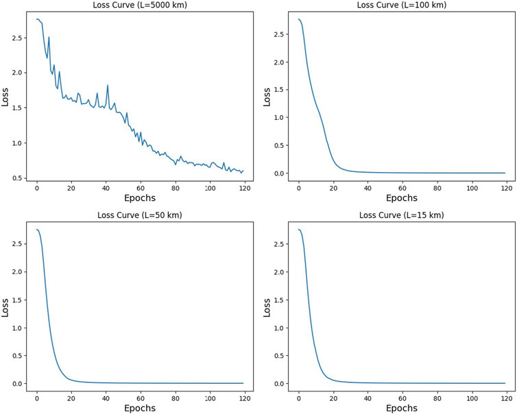
Figure 5. Training loss curves for different optical fiber lengths.

The effect of nonlinearity for different optical fiber lengths, L_o, is shown in Figure 6. The effect of the nonlinear channel on L_o = 5,000 km is shown in Figure 6A. The received constellation is affected by phase noise or phase rotation. The right side of the figure shows the decision regions formed on the basis of the received constellation. When the length is decreased to L_o = 100 km, the nonlinear channel has less impact on the received symbols as compared to L_o = 5,000 km. In other words, the received constellation has less phase noise, and decision regions can easily segregate the received symbols, as shown in Figure 6B. Length is reduced further to L_o = 50 km and L_o = 15 km, as shown in Figure 6C and 6D. The received signal is less affected by the phase noise, and more accurate information is obtained at the receiver side with a reduced symbol error rate. This effect can also be seen in the decision boundaries formed on the received constellation. Therefore, when the fiber length is increased, nonlinearity will affect the received constellation by increasing the phase noise. In other words, received information will be degraded, and the symbol error rate will increase, making it difficult for the receiver to recover the signal information. The symbol error rate on the validation dataset for different optical fibers is shown in Figure 7.

Figure 6

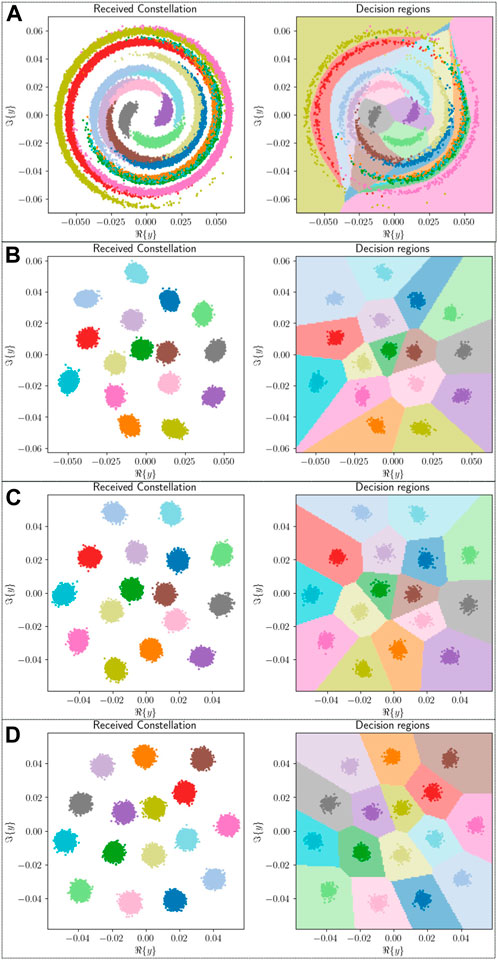
Figure 6. Received constellations and decision regions for different optical fiber lengths. (A) L_o = 5,000 km. (B) L_o = 100 km. (C) L_o = 50 km. (D) L_o = 15 km.

Figure 7

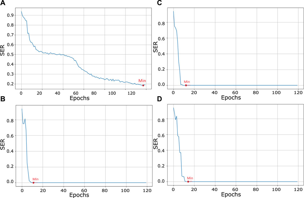
Figure 7. SER on the validation dataset for different optical fiber lengths. (A) L_o = 5,000 km. (B) L_o = 100 km. (C) L_o = 50 km. (D) L_o = 15 km.

4.4 Chromatic dispersion based channel

We consider the effects of chromatic dispersion-based channels on the fiber length. First, a discrete Fourier transform (DFT) is used to convert the original signal into the frequency domain. 16-QAM is used as input. It is fed into the channel, and chromatic dispersion is applied to it. To shift to the time domain (TD), the inverse discrete Fourier transform (IDFT) of the signal is taken. The chromatic dispersion in the TD is given as

$h\left(L_o,t\right)=\sqrt{\frac{c}{jD{\lambda }^2{L}_o}{e}^{j\frac{\pi c}{D{\lambda }^2{L}_o}{t}^2}}.(9)$

In the frequency domain, chromatic dispersion will be

$H\left(L_o,\omega \right)=e^{-j\frac{{\beta }_2{L}_o}{2}{\omega }^2}=e^{j\frac{D{\lambda }^2{L}_o}{4\pi c}{\omega }^2},(10)$

where λ is the light’s wavelength, D is the dispersion coefficient of the optical fiber, β₂ is the group velocity dispersion coefficient, ω is the angular frequency, c is the speed of light, and L_o is the optical fiber length.

To obtain the numerical results, consider D = 17 ps/nm − km, c = 3 × 10⁸ m/s, and P_in = 2 dBm. Table 2 shows the parameters of the NN-based receiver used for the chromatic dispersion-based channel. The model is trained using Keras. During training, the number of Epochs = 50. The loss function known as sparse categorical cross-entropy and optimizer known as Adam [36] are used during the training.

Table 2

Table 2. NN receiver parameters for the chromatic dispersion-based channel.

Chromatic dispersion broadens the signal due to which ISI occurs for different optical fiber lengths, L_o, as shown in Figure 8. The effect of chromatic dispersion when L_o = 100 km is shown in Figure 8A. The received 16-QAM constellation is spread out, and the symbol error rate will increase. When fiber length decreases, the effect of chromatic dispersion on the signal is reduced, as shown for L_o = 75 km in Figure 8B. The signal constellation is less spread out, and ISI is lower. Therefore, the symbol error rate will reduce as the fiber length is reduced. Figures 8C and 8D represent the effect of chromatic dispersion when the propagation distance is further reduced to L_o = 50 km and L_o = 20 km, respectively. It can be seen that the received constellation is slightly affected by the effect of chromatic dispersion. Hence, the spreading of the signal constellation is reduced further, which results in a reduction of the symbol error rate, as compared to L_o = 100 km and L_o = 75 km. To conclude, ISI is reduced by decreasing the fiber length in a chromatic dispersion-based channel, resulting in a reduction of the symbol error rate.

Figure 8

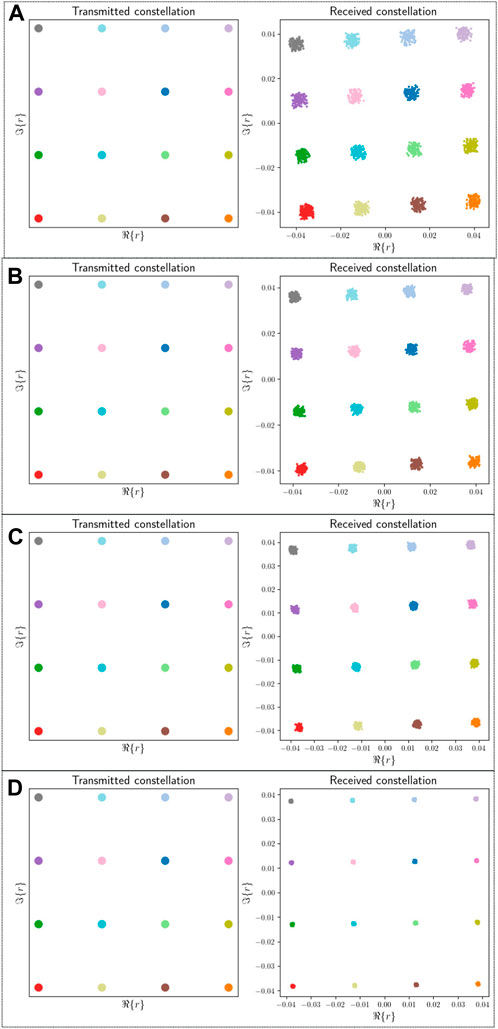
Figure 8. Effect of the chromatic dispersion-based channel for optical fiber lengths. (A) L_o = 100 km. (B) L_o = 75 km. (C) L_o = 50 km. (D) L_o = 20 km.

5 Split-step Fourier method

SSFM is a technique used for simultaneous simulation of self-phase modulation (SPM) and CD in optical fibers. First, nonlinearity alone is applied to the signal in the time domain. After that, the signal is converted into the frequency domain, and CD is applied. Therefore, ∂/∂t in the NLSE is replaced with iω. The signal is converted back into the time domain by taking IDFT. The steps involved in this process can be described as follows [42]:

$X\left(l+k,t\right)=F^{-1}\left[e^{kD\left(i\omega \right)}F\left[e^{kN}X\left(l,t\right)\right]\right],(11)$

where ‘k’ is the small incremental distance and ‘F’ is the fast Fourier transform.

5.1 Iterative and symmetric SSFM

In this technique, dispersion is applied to the signal through half of the distance ‘k’, then nonlinearity acts on the middle of the distance, and finally, dispersion acts again on the remaining half of the distance. The operation is shown as [43]

$X\left(l+k,t\right)=\exp \left(\frac{k}{2}D\right)\exp \left(\frac{N\left(l\right)+N\left(l+k\right)}{2}\right)\exp \left(\frac{k}{2}D\right)X\left(l,t\right).(12)$

Several iterations have to be performed by considering an amplified optical communication system. For each span of the amplifier, dispersion and nonlinearity are mitigated, which leads to high complexity.

5.2 Noniterative asymmetric SSFM

To simplify iterative and symmetric SSFM, an assumption is made that nonlinearity acts only at the beginning of every amplifier. So, for each span, only one iteration is performed. Due to this, the complexity of the system is reduced significantly for the mitigation of nonlinear phase noise [44]. However, the performance of noniterative asymmetric SSFM is 2–3 dB poor compared to iterative SSFM. SSFM has a high computational cost of approximately 105 multiplications per symbol per channel. On the other side, it is a quite powerful simulation technique for mitigating both dispersion and nonlinearity [45].

5.3 Numerical results and discussions

For our numerical simulations, we consider iterative and symmetric split-step Fourier method under different fiber lengths. Consider β₂ = −20 × 10⁻²⁴ s²/km, α = 0.2 dB/km, γ = 1.27 W/km, h = 1 km, and P_in = 1 dBm. Here, β₂ represents the GVD coefficient, nonlinearity coefficient is represented by γ, h is the step size, P_in is the input power, and α is the attenuation. The neural network-based receiver parameters are shown in Table 3. The model is trained using Keras with number of Epochs being 120. A loss function known as sparse categorical cross-entropy is used. Adam optimizer [36] is used for training of the model. The results of different optical fiber lengths, L_o, used in the SSFM-based channel with 16-QAM input, and their decision regions formed are shown in Figure 9.

Table 3

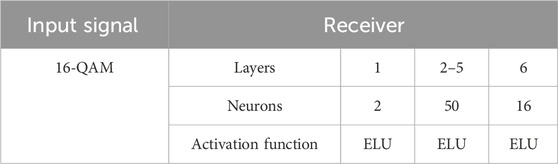
Table 3. NN receiver parameters for the SSFM-based channel.

Figure 9

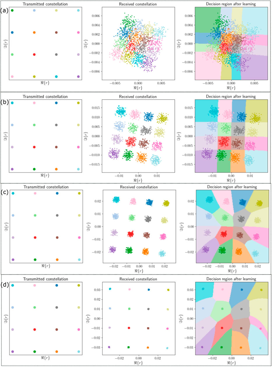
Figure 9. Effect of the split-step Fourier method-based channel for different optical fiber lengths. (A) L_o = 100 km. (B) L_o = 50 km. (C) L_o = 25 km. (D) L_o = 5 km.

Figure 9A shows the effect of the SSFM-based channel for L_o = 100 km. A small portion of the received symbols are intermixed with each other; hence, the symbol error rate will be high. For Figure 9B, the received constellations for L_o = 50 km are forming a boundary with each other, and there is little interference between the received symbols. In Figure 9C, the length is reduced to L_o = 25 km. For this length, the received constellation symbols do not interfere with each other and are some distance apart. Figure 9D shows that for L_o = 5 km, the symbol error rate is minimum compared to other lengths, and received symbols are far apart from each other. Therefore, for short propagation distances, the channel effect on the received constellation is small and the symbol error rate is reduced.

6 Conclusion and future work

The realm of short-reach optical communication has attracted significant attention both within academic circles and industry. Our focus has been on utilizing deep learning models to minimize symbol error rates in these types of optical communication setups. Various channel impairments, such as nonlinearity, CD, and attenuation, need to be accurately modeled. Initially, we addressed the challenge of modeling a nonlinear channel. Although conventional methods exist to tackle this issue, they tend to be intricate. Consequently, we harnessed a deep learning model called autoencoders to facilitate communication over nonlinear channels. This approach enabled the creation of an end-to-end system, yielding promising constellations. Furthermore, we investigated how the inclusion of a nonlinear channel within an autoencoder influences the received constellation as the optical fiber length increases. Another facet of our work involved the deployment of a deep neural network-based receiver utilizing a channel influenced by chromatic dispersion. By gradually extending the optical length, we explored its impact on the received constellation and, consequently, the symbol error rate. Finally, we incorporated the SSFM to emulate the combined effects of nonlinearities, chromatic dispersion, and attenuation in the optical channel. This was accomplished through a neural network-based receiver. The outcome was an evaluation of the symbol error rate as the optical fiber’s length was augmented. Notably, we observed that the symbol error rate increases with the propagation distance of the optical fiber.

The potential for expanding upon this research lies in the application of various machine learning models to further reduce symbol error rates in short-reach optical communication. Although we have employed autoencoders and deep neural network-based receivers (decoders) in our current work, it is worth noting that the channel itself was not modeled using neural networks. To compute gradients in backpropagation, our abovementioned techniques always require a specific channel model. The precise mathematical relationship between the input and output of a real fiber channel is thus unknown, making these approaches inappropriate for real fiber channels. To overcome this limitation, an avenue worth exploring is the integration of reinforcement learning. This approach could enable the optimization of both the transmitter and receiver components independently, without requiring detailed channel knowledge. By leveraging reinforcement learning techniques, we could potentially enhance the overall performance of the system and achieve better symbol error rate outcomes in short-reach optical communication scenarios.

Data availability statement

The raw data supporting the conclusions of this article will be made available by the authors, without undue reservation.

Author contributions

MI: software and writing–original draft. AA: conceptualization and writing–review and editing. AA: writing–review and editing. JM: writing–review and editing. IA: validation and writing–review and editing. SG: methodology, project administration, validation, and writing–review and editing. LP: conceptualization, methodology, and writing–review and editing.

Funding

The author(s) declare that no financial support was received for the research, authorship, and/or publication of this article.

Conflict of interest

The authors declare that the research was conducted in the absence of any commercial or financial relationships that could be construed as a potential conflict of interest.

Publisher’s note

All claims expressed in this article are solely those of the authors and do not necessarily represent those of their affiliated organizations, or those of the publisher, the editors, and the reviewers. Any product that may be evaluated in this article, or claim that may be made by its manufacturer, is not guaranteed or endorsed by the publisher.

References

1. Chagnon M. Optical communications for short reach. J Light Tech Nol (2019) 37:1779–97. doi:10.1109/JLT.2019.2901201

CrossRef Full Text | Google Scholar

2. Chaudhary S, Tang X, Lin B, Wei X. 20Gbps MDM-based optical multimode system for short-haul communication. In: Proceedings of the 2nd International Conference on Algorithms, Computing and Systems; July 27-29, 2018; Beijing, China (2018). doi:10.1145/3242840.3242885

CrossRef Full Text | Google Scholar

3. Kani J-i., Terada J, Hatano T, Kim S-Y, Asaka K, Yamada T Future optical access network enabled by modularization and softwarization of access and transmission functions [Invited]. J Opt Commun Netw (2020) 12:D48–D56. doi:10.1364/jocn.391544

CrossRef Full Text | Google Scholar

4. Satish Kumar M, Rajan M, Sushank C, Faisel T, Raad R. Developing cost-effective and high-speed 40 gbps FSO systems incorporating wavelength and spatial diversity techniques. Front Phys (2021) 9. doi:10.3389/fphy.2021.744160

CrossRef Full Text | Google Scholar

5. Zhong K, Zhou X, Huo J, Yu C, Lu C, Lau APT Digital signal processing for short-reach optical communications: a review of current technologies and future trends. J Light Technol (2018) 36:377–400. doi:10.1109/jlt.2018.2793881

CrossRef Full Text | Google Scholar

6. Karanov B, Chagnon M, Aref V, Ferreira F, Lavery D, Bayvel P, et al. Experimental investigation of deep learning for digital signal processing in short reach optical fiber communications. In: 2020 IEEE Workshop on Signal Processing Systems (SiPS); 20-22 October 2020; Coimbra, Portugal. IEEE (2020). p. 1–6.

CrossRef Full Text | Google Scholar

7. Yu Y, Che Y, Bo T, Kim D, Kim H Reduced-state mlse for an im/dd system using pam modulation. Opt Express (2020) 28:38505–15. doi:10.1364/oe.410674

PubMed Abstract | CrossRef Full Text | Google Scholar

8. Kalla SCK, Rusch LA Recurrent neural nets achieving mlse performance in bandlimited optical channels. In: 2020 IEEE Photonics Conference (IPC); 10-14 November 2024; Rome, Italy. IEEE (2020). p. 1–2.

Google Scholar

9. Gaiarin S, Pang X, Ozolins O, Jones RT, Da Silva EP, Schatz R, et al. High speed pam-8 optical interconnects with digital equalization based on neural network. In: 2016 Asia Communications and Photonics Conference (ACP); 2-5 November 2016; Wuhan, China. IEEE (2016). p. 1–3.

CrossRef Full Text | Google Scholar

10. Ge L, Zhang W, Liang C, He Z Compressed neural network equalization based on iterative pruning algorithm for 112-gbps vcsel-enabled optical interconnects. J Light Technol (2020) 38:1323–9. doi:10.1109/jlt.2020.2973718

CrossRef Full Text | Google Scholar

11. Katz G, Sadot D Radial basis function network equalizer for optical communication ook system. J Lightwave Technology (2007) 25:2631–7. doi:10.1109/jlt.2007.902109

CrossRef Full Text | Google Scholar

12. Da Ros F, Ranzini SM, Dischler R, Cem A, Aref V, Bülow H, et al. Machine-learning-based equalization for short-reach transmission: neural networks and reservoir computing. In: Proceedings Volume 1171205, Metro and Data Center Optical Networks and Short-Reach Links IV. SPIE (2021). doi:10.1117/12.2583011

CrossRef Full Text | Google Scholar

13. Argyris A, Bueno J, Fischer I Photonic machine learning imple-mentation for signal recovery in optical communications. Sci Reports (2018) 8:8487. doi:10.1038/s41598-018-26927-y

PubMed Abstract | CrossRef Full Text | Google Scholar

14. Ranzini SM, Dischler R, Da Ros F, Bülow H, Zibar D Experi-mental investigation of optoelectronic receiver with reservoir computing in short reach optical fiber communications. J Light Technol (2021) 39:2460–7. doi:10.1109/jlt.2021.3049473

CrossRef Full Text | Google Scholar

15. Katumba A, Yin X, Dambre J, Bienstman P A neuromorphic silicon photonics nonlinear equalizer for optical communications with intensity modulation and direct detection. J Light Technol (2019) 37:2232–9. doi:10.1109/jlt.2019.2900568

CrossRef Full Text | Google Scholar

16. Da Ros F, Ranzini SM, Buelow H, Zibar D Reservoir-computing based equalization with optical pre-processing for short-reach optical transmission. IEEE J Sel Top Quan Electron. (2020) 26:1–12. doi:10.1109/jstqe.2020.2975607

CrossRef Full Text | Google Scholar

17. Li J, Lyu Y, Li X, Wang T, Dong X Reservoir computing based equalization for radio over fiber system. In: 2021 23rd International Conference on Advanced Communication Technology (ICACT); 7-10 February 2021, PyeongChang; South Korea. IEEE (2021). p. 85–90.

CrossRef Full Text | Google Scholar

18. Lukoševiˇcius M, Jaeger H. Reservoir computing approaches to recurrent neural network training. Comput Science Review (2009) 3(3):127–49. doi:10.1016/j.cosrev.2009.03.005

CrossRef Full Text | Google Scholar

19. Deligiannidis S, Bogris A, Mesaritakis C, Kopsinis Y Compen-sation of fiber nonlinearities in digital coherent systems leveraging long short-term memory neural networks. J Light Technol (2020) 38:5991–9. doi:10.1109/jlt.2020.3007919

CrossRef Full Text | Google Scholar

20. Lavania S, Kumam B, Matey PS, Annepu V, Bagadi K Adap-tive channel equalization using recurrent neural network under sui channel model. In: 2015 International Conference on Innovations in In- formation, Embedded and Communication Systems (ICIIECS); 19-20 March 2015; Coimbatore, India. IEEE (2015). p. 1–6.

CrossRef Full Text | Google Scholar

21. Karanov B, Chagnon M, Thouin F, Eriksson TA, Bülow H, Lavery D, et al. End-to-end deep learning of optical fiber communications. J Light Technol (2018) 36:4843–55. doi:10.1109/jlt.2018.2865109

CrossRef Full Text | Google Scholar

22. Li M, Wang D, Cui Q, Zhang Z, Deng L, Zhang M End-to- end learning for optical fiber communication with data-driven channel model. In: 2020 Opto-Electronics and Communications Conference (OECC); 4-8 October 2020; Taipei, Taiwan. IEEE (2020). p. 1–3.

CrossRef Full Text | Google Scholar

23. Talreja V, Koike-Akino T, Wang Y, Millar DS, Kojima K, Parsons K End-to-end deep learning for phase noise-robust multi-dimensional geometric shaping. In: 2020 European Conference on Opti- cal Communications (ECOC); 6-10 December 2020; Brussels, Belgium. IEEE (2020). p. 1–3.

CrossRef Full Text | Google Scholar

24. Karanov B, Chagnon M, Aref V, Lavery D, Bayvel P, Schmalen L Optical fiber communication systems based on end-to- end deep learning. In: 2020 IEEE Photonics Conference (IPC); 10-14 November 2024; Rome, Italy. IEEE (2020). p. 1–2.

Google Scholar

25. O’Shea TJ, Karra K, Clancy TC Learning to communicate: channel auto-encoders, domain specific regularizers, and attention. In: 2016 IEEE International Symposium on Signal Processing and Information Technology (ISSPIT); December 12-14, 2016; Limassol, Cyprus. IEEE (2016). p. 223–8.

Google Scholar

26. O’shea T, Hoydis J An introduction to deep learning for the physical layer. IEEE Trans Cogn. Commun. Netw. (2017) 3:563–75. doi:10.1109/tccn.2017.2758370

CrossRef Full Text | Google Scholar

27. Dörner S, Cammerer S, Hoydis J, Ten Brink S Deep learning based communication over the air. IEEE J Sel Top Signal Process (2017) 12:132–43. doi:10.1109/jstsp.2017.2784180

CrossRef Full Text | Google Scholar

28. Hadi MU, Awais M, Raza M, Khurshid K, Jung H. Neural Network DPD for Aggrandizing SM-VCSEL-SSMF-Based Radio over Fiber Link Performance. Photonics (2021), 8:19. doi:10.3390/photonics8010019

CrossRef Full Text | Google Scholar

29. Schaedler M, Kuschnerov M, Calabr‘o S, Pittal‘a F, Bluemm C, Pachnicke S Ai-based digital predistortion for iq mach-zehnder modulators. In: 2019 Asia Communications and Photonics Conference (ACP); 2-5 November 2019; Chengdu, China. IEEE (2019). p. 1–3.

Google Scholar

30. Schädler M, Böcherer G, Pachnicke S Soft-demapping for short reach optical communication: a comparison of deep neural networks and volterra series. J Light Technol (2021) 39:3095–105. doi:10.1109/jlt.2021.3056869

CrossRef Full Text | Google Scholar

31. Schaedler M, Böcherer G, Pittalà F, Calabrò S, Stojanovic N, Bluemm C, et al. Recurrent neural network soft-demapping for nonlinear isi in 800gbit/s dwdm coherent optical transmissions. J Light Technol (2021) 39(16):5278–86. doi:10.1109/JLT.2021.3102064

CrossRef Full Text | Google Scholar

32. Schaedler M, Calabr‘o S, Pittal‘a F, Bluemm C, Kuschnerov M, Pachnicke S Neural network-based soft-demapping for nonlinear channels. In: Optical Fiber Communication Conference. Optical Society of America; 8–12 March 2020; San Diego, California, United States (2020). p. W3D–2. doi:10.1364/ofc.2020.w3d.2

CrossRef Full Text | Google Scholar

33. Goodfellow I, Bengio Y, Courville A Deep learning. Massachusetts, United States: MIT press (2016).

Google Scholar

34. LeCun Y, Bengio Y, Hinton G Deep learning. nature (2015) 521(7553):436–44. 69. doi:10.1038/nature14539

PubMed Abstract | CrossRef Full Text | Google Scholar

35. Nair V, Hinton GE Rectified linear units improve restricted boltz-mann machines. In: Proceedings of the 27th international conference on machine learning (ICML-10); June 21-24, 2010; Haifa, Israel (2010). p. 807–14.

Google Scholar

36. Kingma DP, Ba J Adam: a method for stochastic optimization (2014).

Google Scholar

37. Chollet F, et al. Keras (2015).

Google Scholar

38. Li S, Häger C, Garcia N, Wymeersch H Achievable information rates for nonlinear fiber communication via end-to-end autoencoder learning. In: 2018 European Conference on Optical Communication (ECOC); September 23-27, 2018; Rome, Italy (2018). p. 1–3. doi:10.1109/ecoc.2018.8535456

CrossRef Full Text | Google Scholar

39. Agrawal G Fiber-optic communication systems. 6. new york: John willey & son (2002).

Google Scholar

40. Keykhosravi K, Durisi G, Agrell E A tighter upper bound on the capacity of the nondispersive optical fiber channel. In: 2017 European Conference on Optical Communication (ECOC); 17-21 September 2017; Gothenburg, Sweden. IEEE (2017). p. 1–3.

CrossRef Full Text | Google Scholar

41. Ho K-P Phase-modulated optical communication systems. Cham: Springer Science & Business Media (2005).

Google Scholar

42. Kylemark P Nonlinear fiber optical technologies for transmission and amplification (2004).

Google Scholar

43. Agrawal GP Nonlinear fiber optics. In: Nonlinear science at the dawn of the 21st century. Cham: Springer (2000). p. 195–211.

Google Scholar

44. Ip E, Kahn JM Compensation of dispersion and nonlinear impairments using digital backpropagation. J Light Technol (2008) 26:3416–25. doi:10.1109/jlt.2008.927791

CrossRef Full Text | Google Scholar

45. Ip E, Kahn J Increasing optical fiber transmission capacity beyond next-generation systems. In: LEOS 2008-21st Annual Meeting of the IEEE Lasers and Electro-Optics Society; 9-13 November 2008; Newport Beach, USA (2008). doi:10.1109/leos.2008.4688764

CrossRef Full Text | Google Scholar