 Tomas Fischer
 Sebastian Hainzl
- 1Institute of Hydrogeology, Engineering Geology and Applied Geophysics, Faculty of Science, Charles University, Prague, Czechia
- 2Physics of Earthquakes and Volcanoes, GFZ German Research Centre for Geosciences, Potsdam, Germany
Migration of hypocenters is a common attribute of induced injection seismicity and of earthquake swarms, which distinguishes them from aftershock sequences. Spreading of the triggering front is often examined by fitting the time dependence of hypocenter distances from the origin by the pore pressure diffusion model. The earthquake migration patterns however often exhibit not only spreading envelopes but also fast-growing streaks embedded in the overall migration trends. We review the observed migration patterns and show that in the case of earthquake-driven migration, where the new ruptures are triggered at the edge of previous ruptures, it is more suitable to examine the cluster growth as a function of the event index instead of time. We propose a model that relates the speed of seismicity spreading to the average rupture area and the effective magnitude of the hypocenter cluster. Application of the model to selected linearly growing clusters of the 2008 West Bohemia swarm gives an almost linear increase of the measured total rupture area with the event index, which fits the proposed model. This is confirmed by a self-similar scaling of the average rupture area with the effective magnitude for stress drops ranging from 0.1 to 1 MPa. The relatively small stress drop level indicates the presence of voids along the fault plane and a possible role of aseismic deformation.
1 Introduction
The spreading of earthquake hypocenters is generally considered to be characteristic of earthquake swarms, which distinguishes them from aftershock sequences. While swarms typically show a clear hypocenter migration starting from a single point of the fault plane, aftershocks usually occur immediately all over the fault plane and along the edges of mainshock rupture. First aftershocks are located close to the rupture plane of the mainshock, while later aftershocks sometimes seem to migrate away from the mainshock (Rydelek and Sacks, 2001) at velocities smaller than 1 km/h. A significant expansion of aftershock clouds is only expected in the presence of aseismic processes such as mainshock-induced afterslip (Peng and Zhao, 2010; Perfettini et al., 2019), while coseismic stress transfer of the aftershocks itself can only explain a minor spreading (Helmstetter et al., 2003).
Hypocenter migration of earthquake swarms is generally attributed to fluid flow along the fault plane. Number of examples of swarms from various tectonic environments show this feature, e.g. in Iceland (Woods et al., 2019), Japan (Yoshida and Hasegawa, 2018a), Afar Rift (Wright et al., 2012), Yellowstone (Massin et al., 2013), or West Bohemia/Vogtland (Fischer et al., 2014). Different migration scenarios are observed from monotonous migration in the horizontal or vertical direction or migration with direction changes within the evolution of the seismic cluster. The migration is often attributed to dyke intrusion, hydrofracture propagation, slow slip events, or pore pressure diffusion. Those models will be discussed below.
Monotonous hypocenter migration is also observed for microearthquakes accompanying hydraulic fracturing, which is commonly used in the industry to create a permeable channel in tight rocks in order to increase the production of oil and gas or facilitate water circulation in the geothermal heat exchanger. The hydraulic fracture is formed by massive water injection at pressures exceeding the minimum principal stress. The growth of the edge of the hydrofracture (so-called rupture triggering front) can be explained by the conservation law relating the injected fluid volume to the volume of the fracture (Fischer et al., 2008; Shapiro, 2015). Accordingly, depending on the hydrofracture geometry, either linear or parabolic growth is observed.
Pronounced migration of epicenters of nonvolcanic tremors, the weak seismic signals associated with slow slip on fault planes, has been observed in subduction zones along distances above 100 km, e.g. (Houston et al., 2011). The observed hypocenter patterns are explained by slow slip initiated by pressurization by fluids interacting with small asperities, which is reproduced by model simulations (Luo and Ampuero, 2017). In many cases, the coordinate-time plots of the migrating hypocenters show two features: slow nonlinear growth of the overall envelope and rapid growth of linear streaks during bursts of activity as observed e.g. within the 2008 West Bohemia swarm (Figure 1A). Here, a streak is defined as a narrow linear belt of points in the coordinate-time plot, which is usually embedded in the overall large-scale migration of the seismic cloud. We identified similar rapidly propagating streaks also in other swarms from West Bohemia and other areas as Yellowstone (Shelly et al., 2016) or Corinth Rift (Kapetanidis et al., 2015). Interestingly, similar streaks also occur during the nonvolcanic tremors showing both forward and reverse motion of epicenters at velocities from 7 to 100 km/day (Ghosh et al., 2010; Houston et al., 2011) (see Figure 2 in Ghosh et al., 2010). In contrast to the natural earthquakes, the seismicity evolution with time is quite smooth and in most cases no streaks of hypocenters are apparent for the injection-induced seismicity (Figure 1G). The only observation of a feature similar to the rapid streaks is that of Shapiro and Dinske, 2009, who attributed the linear fronts in the distance-time plots to hydraulic fracture opening.
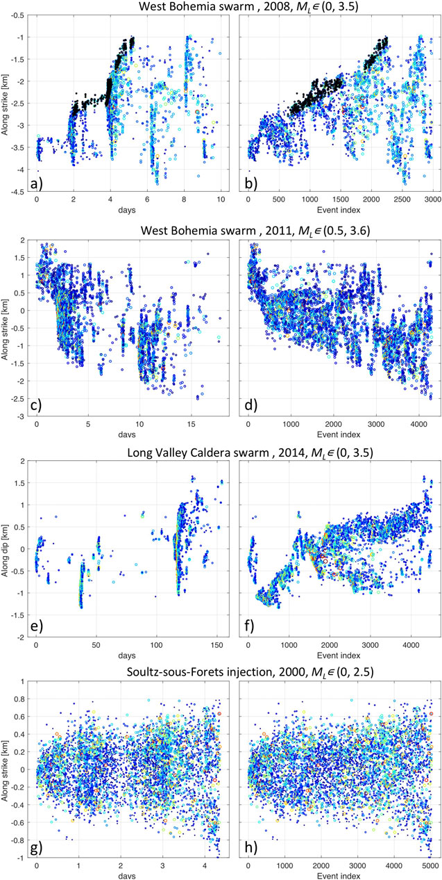
FIGURE 1. Migration of various types of seismicity for three cases of swarm activity (A–C) and one case of injection-induced seismicity (D). Coordinate-time plots (left panels) and coordinate–event-index plots (right panels) for the West-Bohemian swarm in 2008 (A), in 2011 (B), Long-Valley Caldera swarm in 2014 (C) and Soultz-sous-Forets injection in 2000. Note the episodic occurrence of activity in the coordinate-time plots compared to the overall continuous spreading of activity in the coordinate-event-index plots. Note also that fast propagating streaks of hypocenters are observed in swarms but are missing in the injection induced seismicity. The color of symbols from dark blue to dark red is proportional to the event magnitude. In (A) two spreading episodes are highlighted in black in both coordinate-time and coordinate-event-index plots.
In summary, seismic swarms and nonvolcanic tremors show migration patterns on two scales: 1) an (asymmetric) overall growth over days to weeks 2) rapid migration on small spatial and temporal scales, partially with reversed trends. While the overall growth is to be explained either by pore pressure diffusion or hydraulic fracture growth (possibly also by slow slip, but not analyzed in detail yet), the embedded rapid migration have been studied only rarely in detail. Yoshida and Hasegawa (2018b) analyzed the triggering of the Sendai-Okura earthquake swarm by the 2011 Tohoku-Oki earthquake. And recently, Dublanchet and Barros (2020) proposed a model that reproduces the dual migration speeds observed in real swarms by coupling rate-and-state friction, non-linear diffusivity and elasticity along the fault.
Regarding the control of seismicity migration, two end-member cases can be distinguished: externally (aseismic) and internally (seismic) controlled propagation. In the first case an external physical process drives and controls the migration, where earthquakes are only passive markers of this usually time-dependent process. This could be pore-pressure diffusion (Shapiro et al., 1997), hydraulic fracture growth (Dahm et al., 2010), or slow slip (Schwartz and Rokosky, 2007). In the second case, the migration is self-controlled by the earthquake ruptures themselves in the way that the ruptures allow or facilitate nucleation of adjacent new ruptures. Such an earthquake-induced effect can be related to coseismically induced elastic stress changes as well as postseismic effects such as creation of pore-space enabling subsequent fluid flow. Both increase the stress state at the rupture borders facilitating subsequent adjacent ruptures. In such a case, the internal processes and conditions control the “time” and no general time dependence of the seismicity migration is necessarily expected.
In this paper, we review the existing approaches to understanding the earthquake migration. We show examples of migration of earthquake swarms, where both the slow growth of the triggering front and the fast propagation of streaks occur, in particular when displayed using the coordinate - event order plot. Provided that every rupture opens the way for nucleation of the further rupture, we develop a theoretical model of the seismicity spreading related to the source parameters of the earthquakes suitable for the physical interpretation of the observed migration patterns.
2 Models and Interpretation of Earthquake Migration
In the following, we review the existing approaches for interpreting and employing the spreading of earthquake hypocenters.
2.1 Pore Pressure Diffusion
The observed hypocenter migration shows, in many cases, a non-linear growth of envelope in the distance-time plot, which is commonly interpreted by pore pressure diffusion in a homogeneous isotropic medium. The model was originally proposed to interpret the spreading of hypocenters of injection-induced seismicity (Shapiro et al., 1997). It is based on the assumption that earthquakes map the advance of the pore pressure front. It is also assumed that the diffusivity of the rock is constant and that the pore pressure field is decoupled from seismic rupturing and related stress changes. This is in contrast to, for example, the model of Yamashita (1999) where the effect of dynamic pore creation is considered. Ignoring such coupling effects, the evolution of the pore-pressure field can be described by the diffusion equation whose solution for a point pressure source gives the distance r of the propagating pore pressure front as
Rock properties are, however, anisotropic because of strong heterogeneities like faults acting as permeable channels on the one hand, or as impermeable barriers on the other hand. Furthermore, the stress field is heterogeneous due to the stress gradients originating from density contrasts between fluid and rock or heterogeneous tectonic stress. The combination of both types of heterogeneities necessarily results in the preferred orientation of the fluid flow. Consequently, the seismicity front is expected to depend on the direction. The data of West-Bohemia/Vogtland swarms show a clear directional dependence of earthquake migration. In the case of the 2008 swarm the migration in dip-direction could be very well fitted by the pore pressure front curves. However, it requires different hydraulic diffusivities for up-dip and down-dip directions. The estimated down-dip diffusivity (
2.2 Hydraulic Fracture Growth
The pore pressure diffusion model is only appropriate in the limit of poroelasticity, which means, if non-linear effects such as the creation of pore-volume can be neglected and hydraulic properties remain unchanged. If the involved fluid pressure exceeds the minimum confining pressure, hydrofracturing of intact rock takes place. This leads locally to open channels for fluid transport and thus strongly changes the local permeability and hydraulic properties. As a result, instead of pore pressure diffusion in isotropic intact medium, the high-pressure fluid injection results in a subsequent opening of the fault zone and related fluid flows that are driven, in addition to the injection itself, by stress gradients. In a homogeneous rock a hydraulic fracture should open against the direction of the minimum stress component
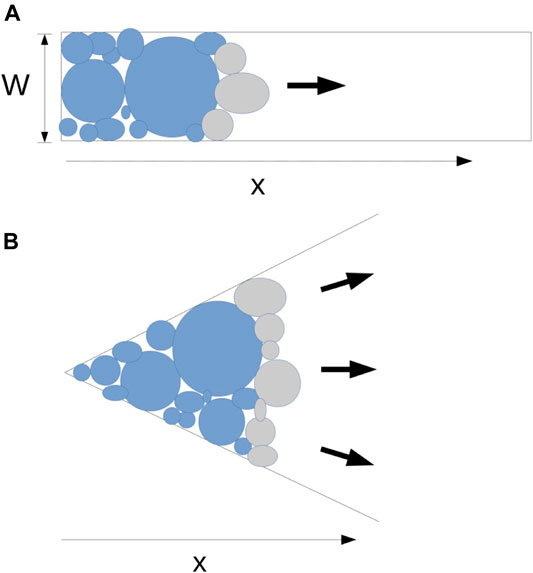
FIGURE 2. Schematic illustration of seismicity model growth supposing that a new rupture is initiated at the edge of the previous rupture. (A) The channel growth (model C) is related to a unidirectional or bidirectional 1-D advance of the rupture front. (B) The sector growth (model S) considers a 2-D advance of the rupture front.
2.3 Slow Slip Driven Seismicity
In contrast to the two other mechanisms, slow slip describes transient aseismic shear dislocation (slip) on faults. By means of new geodetic instrumentation, slow slip events have been identified to occur frequently on faults (Schwartz and Rokosky, 2007). Particularly, it is expected to occur in fault zones, where frictional behavior is partly characterized by velocity strengthening. However, it can also occur in velocity weakening zones, if the nucleation dimension exceeds the asperity size. The nucleation size is itself inversely proportional to the effective normal stress, thus the evaluated pore pressure favors aseismic vs. coseismic slip (Dieterich, 2007). While aseismic slip events can nucleate spontaneously, they can also be triggered by fluid injection (Guglielmi et al., 2015) or coseismic slip. The latter is known as afterslip which is believed to be one of the main drivers for aftershocks (Perfettini et al., 2019). In particular, a
2.4 Effective Stress Drop Concept
Fischer and Hainzl (2017) proposed to employ the spreading of hypocenters of earthquake clusters for interpreting the stress release of the involved seismicity. The basic idea is that if a large earthquake rupture is replaced by numerous small ruptures, which is the mainshock on the one hand and the earthquake swarm on the other hand, similar strain should be released in both cases. Then the total seismic moment of the cluster should equal the seismic moment of a single large event and the familiar formula for seismic moment of a circular rupture
3 Identification of Migration Patterns
Typically, migration patterns are analyzed in the distance-time domain, where the form of observed migration patterns also depends on definition of distance. Traditionally, the dependence of unsigned distance on time,
An additional analysis tool is to use the event order as the independent variable, which is also termed natural time (Rundle et al., 2018). In such a case, a coordinate-event-index plot
The form of migration diagrams using the coordinate-time plot and coordinate-event-index plot is compared in the left and right panels of Figure 1 for selected swarm activities. In the coordinate-event-index plots the periods of quiescence disappear and the original temporal clusters apparent in the coordinate-time plot merge into a continuous seismicity sequence migrating in a single dominating direction. The triggering front shows a linear envelope whose slope (migration velocity measured in meters per event) stays almost constant for longer periods. Note the continuous seismicity growth of the 2008 West-Bohemia swarm in the event-index plot (Figure 1B) compared to the heavily interrupted spreading in the time plot (Figure 1A) of the same activity. The change of growth character is highlighted in two rupture front clusters, which are continuous in the coordinate-event-index plot, but strongly discontinuous in the coordinate-time plot. Similar characteristics are illustrated in Figures 1E,F for the 2014 swarm in the Long Valley Caldera (Shelly et al., 2016), which showed, compared to the 2008 West-Bohemia swarm, almost simple unilateral spreading. The plots in Figure 1 also illustrate the two aforementioned phenomena: the overall growth of the seismic clouds manifested in the triggering front envelope and embedded rapid streaks that propagate both in the same and opposite directions as the triggering envelope.
4 Theoretical Model
One end-member model considers earthquakes only as a passive result of an underlying driving force, e.g. pore-pressure diffusion or slow slip which is not influenced by the triggered earthquakes. In this case, the analysis of the distance-time or coordinate-time plots is sufficient to characterize the migration pattern and the underlying process. However, in the other end-member model, earthquake migration is only possible due to the occurrence of earthquakes, e.g. by the creation of pore-space during ruptures. The presence of clear triggering fronts and embedded linear streaks in the coordinate-event-index plots, while no clear migration pattern can be observed in the coordinate-time plot, points to the latter case. In particular, in such a case, the speed of growth should increase with the size of the event ruptures. Developing a theoretical model for the earthquake generation in the case of a self-driven seismicity migration would help understand the generation mechanism of earthquake swarms.
In accordance with the Yamashita (1999) model we suppose that every rupture facilitates the nucleation of adjacent ruptures. This can be simplified by assuming that subsequent events are without overlap initiated at the outer border of the previous rupture. In two dimensions, two geometrical concepts are considered, the channel (C) model describing a unilateral growth along a channel of width W and the sector (S) model describing a two-dimensional sectorial growth with angle θ (Figure 2).
The speed of the cluster growth is then related to the average position x of the rupture front, which is after the occurrence of N events (as observed in Figure 1) simply given by
where both constants ν and D are proportional to the average rupture area
In order to express
We also use the relation between the area A of a circular rupture and seismic moment
leads to
where f is a geometric factor of the source model,
Then, the average rupture area
In the above equations,
Then Eq. 1 describes the average position of the seismicity as a function of observed events
are used instead of ν and D, respectively.
5 Application to the Seismicity Data
Equation (6) predicts the average rupture area
Based on
As follows from Eq. 6, the average rupture
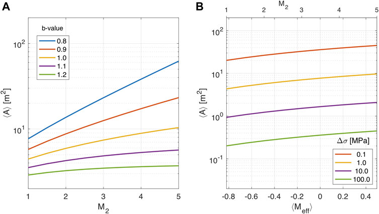
FIGURE 3. Average rupture area
As predicted by Eq. 6, except the case
The curves in Figure 3 predict the average rupture area
To test the validity of the presented models on data we measure the growth of selected clusters of the 2008 swarm in West Bohemia, whose migration patterns are presented in Figure 1 and compare it with theoretical
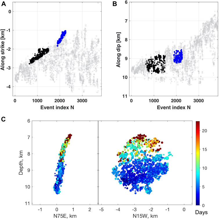
FIGURE 4. The 2008 earthquake swarm in West-Bohemia showed prevailing unidirectional growth of the seismicity front in the strike-ward (A) and upward (B) directions. Two linearly growing clusters were selected in the strike direction for the analysis. The triggering front of the earlier cluster (black) growed slower than that of the later cluster (blue). To measure the distance between the points needed for removing outliers, the event index was transformed into a distance in km so that the aspect ratio of the diagram was 1:1. In (C), two vertical sections show the planar character of the swarm activity; the symbol color is proportional to the event origin time.
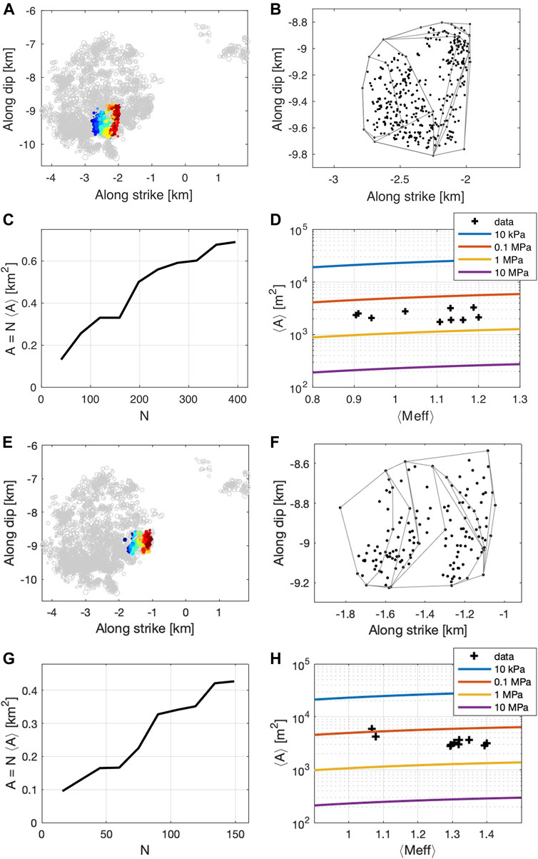
FIGURE 5. Growth analysis of the two clusters of the 2008 West-Bohemia swarm identified in Figure 4: The activated area is marked in colors, which are proportional to the event index (A,E); its convex hull was determined (B,F) for extending equidistant windows that included from 10 to 100% of events; the scaling of the total rupture area with the number of events is almost linear (C,D). The dependence of the average rupture area per event
The total rupture area was measured by the convex envelope algorithm (convhull) implemented in Matlab, which determines the smallest total area A that contains the hypocenter projections within a convex hull. To track the cluster growth, we determine the ruptured area for an increasing number of events; 10 equidistant steps were used. The panels b and f of Figure 5 show the growing convex hull of the clusters indicating a mixed channel and sector growth. The dependence of the measured total rupture area on the number of included events is shown in panels c and g of Figure 5 indicating an approximately linear increase of the area with event index, which is in agreement with the model prediction in Eq. 2. The average rupture area per event
Scaling between the average rupture area and the measured average effective magnitude of the two clusters is analyzed in panels d and h of Figure 5. The measured
For the moment-magnitude relation (Eq. 4) we used constants
6 Discussion and Conclusions
Our analysis shows that the usage of coordinate-event-index plots can yield valuable insights into the earthquake triggering process. However, it is important to note that this analysis should always be performed in conjunction with an analysis of traditional coordinate-time plots. A linear growth with the event-index does not necessarily mean that the migration process is internally driven. In the case that earthquakes are triggered in a homogeneously pre-stressed brittle fault segment by external forcing such as pore-pressure diffusion, the earthquake number would be expected to increase with the pressurized area. Thus, even if the events do not influence each other, this would lead to a linear or square-root growth with earthquake index, similarly to the case of self-driven migration. However, in the case of diffusion-driven seismicity, the space-time plots would also show a clear and continuous migration pattern. In contrast, the space-time plots are expected to show a less clear picture with discontinuous spreading in the case of self-driven migration, as observed for our analyzed cases (see Figure 1). Only the combined analysis of space-time and space-index plots together can resolve this issue.
The graphs in Figure 5 show that the total ruptured area grows almost linearly with the event index, as expected for the suggested model supposing that every rupture facilitates the nucleation of a new adjacent rupture making the seismogenic process self-organized. The local shape of the
Another worth-noting point is the estimated stress drop of less than 1 MPa, which appears rather small compared to the estimated static stress drops of individual events of the West-Bohemia swarms in the order of 10 MPa (Michalek and Fischer, 2013). It is of interest to note that using the concept of effective stress drop (Fischer and Hainzl (2017)), we arrived at a similar value of
Migration characteristics are used to typify seismic activity. In contrast to the random occurrence of aftershock hypocenters along the mainshock fault plane, earthquake swarms and injection-induced seismicity outstand by monotonous migration resulting in the spreading of the hypocenter cloud. This is usually attributed to fluid flow along the fault plane, which could be modeled by pore-pressure diffusion or by a propagating hydraulic fracture. In this end-member case, the aseismic load leads to an increase of the effective stress in an expanding volume which triggers the earthquake migration as function of time, independently of precursory seismicity. Earthquakes are assumed to be triggered in this case in critically loaded areas, where stresses or pore pressure is elevated due to the aseismic driving process. As a result, void areas may occur in the diffusion model, which are bridged by the aseismic pore pressure diffusion or hydrofracture growth. Accordingly, the event coordinates would grow non-linear, respectively jump with increasing event index, which would also apply to the growth of average rupture area with the event index. This would result in low values of the estimated stress drop due to the large activated area and small strain released in a brittle way, as discussed in detail in our previous study (Fischer and Hainzl, 2017). However, the suggested analysis of the coordinate-event-index plots would indicate that aseismic deformation is present in this case due to the non-linear, jump-type shape of the rupture front.
In contrast to the models where the seismicity is externally controlled by the underlying time-dependent aseismic process, the seismicity is self-controlled by the rupture occurrences in the other end-member case of self-driven migration. In that case, fluid flow is only a secondary process where seismic slip allows the fluid to migrate into the reactivated fracture through dilatancy, and once the pressure gets high enough on the rupture edge, the subsequent rupture occurs. Consequently, it is the rupture occurrence that measures the time and, hence, it is more suitable to use the event index as an independent variable when exploring the seismicity migration. A continuous, and in most cases linear advance of rupture front is predicted in the coordinate-event-index plot in the case of self-driven earthquake migration.
For several examples of seismic swarms, we show how the form of migration plots changes when the event index is used instead of time. Discontinuous activities convert to continuous ones and nonlinear growth with time becomes linear when the event index is displayed on the horizontal axis. We interpret this behavior by a model supposing that every rupture opens the way for nucleation of the further one. Then the speed of growth is proportional to the average rupture area of the earthquakes that is related to the magnitude-frequency distribution of the events and the stress drop.
Our test using relocations of the 2008 earthquake swarm in West-Bohemia confirms the validity of the presented model. The two selected clusters, which represent the linearly spreading triggering front in the coordinate-event-index plot, show an almost linear growth of the total rupture area with the event index. Based on the envelopes of the observed hypocenters, the estimated speed of growth is 2.4 and 4.6 m per event and the average rupture area of the cluster events is 1750 m2 and 2,870 m2 for the two clusters, respectively. The observed difference in the spatial spreading speed is explained by differences in the frequency-magnitude distribution, which is expressed by the different effective magnitudes of 1.1 and 1.4 for the two clusters, respectively. The average speed measured in time domain is 340 m/day for the first cluster and 720 m/day for the second cluster. The dependence of average rupture areas on the effective magnitude points to self-similar scaling with stress drops ranging between 0.1 and 1 MPa. Although our analysis indicates a self-driven cluster growth, the low stress drops might indicate that parts of the rupture area deformed aseismically either by pore-pressure induced or seismically triggered creep and did not contribute to the seismic moment release. In future studies, we will address the role of fluids and earthquake ruptures for specific migration patterns such as triggering fronts and embedded linear streaks in the case of various seismic activities in more detail.
Data Availability Statement
The datasets presented in this study can be found in online repositories. The names of the repository/repositories and accession number(s) can be found below: https://zenodo.org/record/4294887.
Author Contributions
TF and SH developed the idea of linear streaks and wrote the manuscript. TF contributed to the theory developed by SH and carried out the data analysis.
Funding
The work of TF was supported by the Czech Funding Agency under the grant 20-26018S.
Conflict of Interest
The authors declare that the research was conducted in the absence of any commercial or financial relationships that could be construed as a potential conflict of interest.
Supplementary Material
The Supplementary Material for this article can be found online at: https://www.frontiersin.org/articles/10.3389/feart.2021.638336/full#supplementary-material.
Acknowledgments
We are grateful to Josef Vlček for help with preparing the code for the cluster identification and Martin Bachura for providing the relocated hypocenters. We also thank the editor Pascal Audet and two reviewers for their very helpful comments.
Appendix
Average rupture area
Given the probability density function of the Gutenberg-Richter distribution (Eq. 3) and the relation between rupture area A and earthquake magnitude m (Eq. 5), the average rupture area can be determined as
For
References
Brune, J. N. (1970). Tectonic stress and the spectra of seismic shear waves from earthquakes. J. Geophys. Res. 75, 4997–5009. doi:10.1029/jb075i026p04997
Dahm, T., Hainzl, S., and Fischer, T. (2010). Bidirectional and unidirectional fracture growth during hydrofracturing: role of driving stress gradients. J. Geophys. Res. 115, B12322. doi:10.1029/2009jb006817
Dieterich, J. H. (2007). Applications of rate- and state-dependent friction to models of fault-slip and earthquake occurrence. Treatise Geophys. (Elsevier) 4, 93–110. doi:10.1016/b978-0-444-53802-4.00075-0
Dublanchet, P., and Barros, L. D. (2020). Stress‐dependent b value variations in a heterogeneous rate‐and‐state fault model. Geophys. Res. Lett. 47, e2020GL090025. doi:10.1029/2020gl087434
Fischer, T., Hainzl, S., and Dahm, T. (2009). The creation of an asymmetric hydraulic fracture as a result of driving stress gradients. Geophys. J. Int. 179, 634–639. doi:10.1111/j.1365-246x.2009.04316.x
Fischer, T., and Hainzl, S. (2017). Effective stress drop of earthquake clusters. Bull. Seism. Soc. Am. 107, 2247–2257. doi:10.1785/0120170035
Fischer, T., Hainzl, S., Eisner, L., Shapiro, S. A., and Le Calvez, J. (2008). Microseismic signatures of hydraulic fracture growth in sediment formations: observations and modeling. J. Geophys. Res. 113, B02307. doi:10.1029/2007JB005070
Ghosh, A., Vidale, J. E., Sweet, J. R., Creager, K. C., Wech, A. G., Houston, H., et al. (2010). Rapid, continuous streaking of tremor in cascadia. Geochem. Geophys. Geosyst. 11. doi:10.1029/2010GC003305
Guglielmi, Y., Cappa, F., Avouac, J. P., Henry, P., and Elsworth, D. (2015). INDUCED SEISMICITY. Seismicity triggered by fluid injection-induced aseismic slip. Science 348, 1224–1226. doi:10.1126/science.aab0476
Hainzl, S., Fischer, T., Čermáková, H., Bachura, M., and Vlček, J. (2016). Aftershocks triggered by fluid intrusion: evidence for the aftershock sequence occurred 2014 in West Bohemia/Vogtland. J. Geophys. Res. Solid Earth 121, 2575–2590. doi:10.1002/2015jb012582
Hainzl, S., Fischer, T., and Dahm, T. (2012). Seismicity-based estimation of the driving fluid pressure in the case of swarm activity in western bohemia. Geophys. J. Int. 191, 271–281. doi:10.1111/j.1365-246x.2012.05610.x
Hanks, T. C., and Kanamori, H. (1979). A moment magnitude scale. J. Geophys. Res. 84, 2348–2350. doi:10.1029/jb084ib05p02348
Helmstetter, A., and Sornette, D. (2003). Diffusion of epicenters of earthquake aftershocks, Omori's law, and generalized continuous-time random walk models. Phys. Rev. E Stat. Nonlin Soft Matter Phys. 66, 061104. doi:10.1103/PhysRevE.66.061104
Hiemer, S., Roessler, D., and Scherbaum, F. (2012). Monitoring the west bohemian earthquake swarm in 2008/2009 by a temporary small-aperture seismic array. J. Seismol. 16, 169–182. doi:10.1007/s10950-011-9256-5
Houston, H., Delbridge, B. G., Wech, A. G., and Creager, K. C. (2011). Rapid tremor reversals in cascadia generated by a weakened plate interface. Nat. Geosci. 4, 404–409. doi:10.1038/ngeo1157
Jakoubková, H., Horálek, J., and Fischer, T. (2017). 2014 mainshock-aftershock activity versus earthquake swarms in west bohemia, Czech republic. Pure Appl. Geophys. 175, 109–131. doi:10.1007/s00024-017-1679-7
Kapetanidis, V., Deschamps, A., Papadimitriou, P., Matrullo, E., Karakonstantis, A., Bozionelos, G., et al. (2015). The 2013 earthquake swarm in helike, Greece: seismic activity at the root of old normal faults. Geophys. J. Int. 202, 2044–2073. doi:10.1093/gji/ggv249
Kato, N. (2007). Expansion of aftershock areas caused by propagating post-seismic sliding. Geophys. J. Int. 168, 797–808. doi:10.1111/j.1365-246x.2006.03255.x
Le Calvez, T., Horálek, J., Hrubcová, P., Vavryčuk, V., Bräuer, K., and Kämpf, H. (2014). Intra-continental earthquake swarms in west-bohemia and vogtland: a review. Tectonophysics 611, 1–27. doi:10.1016/j.tecto.2013.11.001
Luo, Y., and Ampuero, J. P. (2017). Tremor migration patterns and the collective behavior of deep asperities mediated by creep. Preprint. doi:10.17605/OSF
Madariaga, R., and Ruiz, S. (2016). Earthquake dynamics on circular faults: a review 1970-2015. J. Seismol. 20, 1235–1252. doi:10.1007/s10950-016-9590-8
Marzocchi, W., and Sandri, L. (2003). A review and new insights on the estimation of the b-value and its uncertainty. Ann. Geophys. 46, 1271–1282. doi:10.4401/ag-3472
Massin, F., Farrell, J., and Smith, R. B. (2013). Repeating earthquakes in the yellowstone volcanic field: implications for rupture dynamics, ground deformation, and migration in earthquake swarms. J. Volcanol. Geoth. Res. 257, 159–173. doi:10.1016/j.jvolgeores.2013.03.022
Michálek, J., and Fischer, T. (2013). Source parameters of the swarm earthquakes in west bohemia/vogtland. Geophys. J. Int. 195, 1196–1210. doi:10.1093/gji/ggt286
Mls, J., and Fischer, T. (2017). A new mathematical model of asymmetric hydraulic fracture growth. Geophys. Prospect. 66, 549. doi:10.1111/1365-2478.12590
Parotidis, M., Shapiro, S. A., and Rothert, E. (2004). Back front of seismicity induced after termination of borehole fluid injection. Geophys. Res. Lett. 31, L02612. doi:10.1029/2003gl018987
Peng, Z., and Zhao, P. (2009). Migration of early aftershocks following the 2004 parkfield earthquake. Nat. Geosci. 2, 877–881. doi:10.1038/NGEO697
Perfettini, H., Frank, W. B., Marsan, D., and Bouchon, M. (2019). Updip and along‐strike aftershock migration model driven by afterslip: application to the 2011 tohoku‐oki aftershock sequence. J. Geophys. Res. Solid Earth 124, 2653. doi:10.1029/2018JB016490
Rundle, J. B., Luginbuhl, M., Giguere, A., and Turcotte, D. L. (2018). Natural time, nowcasting and the physics of earthquakes: estimation of seismic risk to global megacities. Pure Appl. Geophys. 175, 647–660. doi:10.1007/s00024-017-1720-x
Rydelek, P. A., and Sacks, I. S. (2001). Migration of large earthquakes along the san jacinto fault; stress diffusion from the 1857 fort tejon earthquake. Geophys. Res. Lett. 28, 3079–3082. doi:10.1029/2001gl013005
Schwartz, S. Y., and Rokosky, J. M. (2007). Slow slip events and seismic tremor at circum-pacific subduction zones. Rev. Geophys. 45, a. doi:10.1029/2006RG000208
Shapiro, S. (2015). Fluid-induced seismicity. Cambridge, United Kingdom: Cambridge University Press.
Shapiro, S. A., and Dinske, C. (2009). Fluid-induced seismicity: pressure diffusion and hydraulic fracturing. Geophys. Prospect. 57, 301–310. doi:10.1111/j.1365-2478.2008.00770.x
Shapiro, S. A., Huenges, E., and Borm, G. (1997). Estimating the crust permeability from fluid-injection-induced seismic emission at the ktb site. Geophys. J. Int. 131, F15–F18. doi:10.1111/j.1365-246x.1997.tb01215.x
Shelly, D. R., Ellsworth, W. L., and Hill, D. P. (2016). Fluid-faulting evolution in high definition: connecting fault structure and frequency-magnitude variations during the 2014 long valley caldera, California, earthquake swarm. J. Geophys. Res. Solid Earth 121, 1776–1795. doi:10.1002/2015jb012719
Woods, J., Winder, T., White, R. S., and Brandsdóttir, B. (2019). Evolution of a lateral dike intrusion revealed by relatively-relocated dike-induced earthquakes: the 2014-15 Bárðarbunga-Holuhraun rifting event, Iceland. Earth Planet. Sci. Lett. 506, 53–63. doi:10.1016/j.epsl.2018.10.032
Wright, T. J., Sigmundsson, F., Pagli, C., Belachew, M., Hamling, I. J., Brandsdóttir, B., et al. (2012). Geophysical constraints on the dynamics of spreading centres from rifting episodes on land. Nat. Geosci, 5, 242. doi:10.1038/NGEO1428
Yamashita, T. (1999). Pore creation due to fault slip in a fluid-permeated fault zone and its effect on seismicity: generation mechanism of earthquake swarm. Pure Appl. Geophys. 155, 625–647. doi:10.1007/978-3-0348-8677-2_19
Yoshida, K., and Hasegawa, A. (2018a). Hypocenter migration and seismicity pattern change in the yamagata-fukushima border, NE Japan, caused by fluid movement and pore pressure variation. J. Geophys. Res. Solid Earth 123, 5000–5017. doi:10.1029/2018jb015468
Yoshida, K., and Hasegawa, A. (2018b). Sendai-okura earthquake swarm induced by the 2011 tohoku-oki earthquake in the stress shadow of ne Japan: detailed fault structure and hypocenter migration. Tectonophysics 733, 132–147. doi:10.1016/j.tecto.2017.12.031
Keywords: Statistical seismology, fluid induced seismicity, earthquake source observations, earthquake interaction, seismicity migration
Citation: Fischer T and Hainzl S (2021) The Growth of Earthquake Clusters. Front. Earth Sci. 9:638336. doi: 10.3389/feart.2021.638336
Received: 06 December 2020; Accepted: 29 January 2021;
Published: 17 March 2021.
Edited by:
Pascal Audet, University of Ottawa, CanadaReviewed by:
Keisuke Yoshida, Tohoku University, JapanLouis De Barros, UMR7329 Géoazur (GEOAZUR), France
Copyright © 2021 Fischer and Hainzl. This is an open-access article distributed under the terms of the Creative Commons Attribution License (CC BY). The use, distribution or reproduction in other forums is permitted, provided the original author(s) and the copyright owner(s) are credited and that the original publication in this journal is cited, in accordance with accepted academic practice. No use, distribution or reproduction is permitted which does not comply with these terms.
*Correspondence: Tomas Fischer, ZmlzY2hlckBuYXR1ci5jdW5pLmN6