The Last Glacial Maximum and Deglacial History of the Seno Skyring Ice Lobe (52°S), Southern Patagonia

There are still many uncertainties about the climatic forcing that drove the glacier fluctuations of the Patagonian Ice Sheet (PIS, 38–55°S) during the last glacial period. A key source of uncertainty is the asynchrony of ice lobe fluctuations between the northern, central, and southern PIS. To fully understand the regional trends requires careful mapping and extensive geochronological studies. This paper presents geomorphological and geochronological reconstructions of the glacial and deglacial landforms formed during the last glacial period at the Seno Skyring lobe, southernmost Patagonia (52°S, 71°W). We present a detailed geomorphological map, where we identify two moraine systems. The outer and older is named Laguna Blanca (LB) and the inner Río Verde (RV). The LB moraines were built subaerially, whereas parts of the RV were deposited subaqueously under the palaeo lake Laguna Blanca, which developed during deglaciation. We conducted surface exposure ¹⁰Be dating methods on boulder samples collected from LB and RV glacial margins. The moraine LB III and LB IV formed at 26.3 ± 2.3 ka (n = 5) and 24.3 ± 0.9 ka (n = 3), respectively. For the inner RV moraine, we obtained an age of 18.7 ± 1.5 ka (n = 6). For the palaeo Laguna Blanca evolution, we performed ¹⁰Be exposure ages on shoreline berms and optically stimulated luminesce dating to constrain the lake levels, and ¹⁰Be depth profile dating on an outwash deposit formed by a partial lake drainage event, which occurred at 22 ± 3 ka. For the RV moraine deglaciation, we performed radiocarbon dating of basal sediments in a peat bog, which indicates that the glacier retreated from the terminal RV moraine by at least c. 16.4 cal kyr BP. Our moraine geochronology shows an asynchrony in the maximum extents and a different pattern of ice advances between neighbouring lobes in southern Patagonia. We speculate that this may be due, at least in part, to the interaction between topography and the precipitation carried by the southern westerly wind belt. However, we found broad synchrony of glacial readvances contemporaneous with the RV moraine.

1 Introduction

The location of Patagonia in the Southern Hemisphere makes it a good location to study paleoclimate of the Southern Hemisphere since it is the only continental region that straddles the core of the Southern Westerly Winds (SWWs; Figure 1A), which are directly linked with the precipitation and temperatures affecting the region (Garreaud, 2009). Moreover, its close position to Antarctica allows comparisons between the terrestrial and marine records from Patagonia with Antarctic climatic proxies (Sugden et al., 2009; Darvill et al., 2016; García et al., 2020). The last glacial cycle was marked by a number of cold intervals, according to Antarctic ice cores (Jouzel et al., 2007). However, these events are not consistently represented in the glacial geomorphology of the Patagonian Ice Sheet (PIS) margin (Davies et al., 2020). Terrestrial geochronologic records show that the maximum extents of the ice lobe fluctuations along the PIS occurred at different times during the last glacial period, suggesting an asynchrony between northern, central and southern Patagonia. Most moraine chronologies have recorded local ice maxima during MIS 2 and MIS 3, but also MIS 4 and MIS 5a (Kaplan et al., 2004; Douglass et al., 2006; Hein et al., 2010; Darvill et al., 2015; García et al., 2018, 2021; Mendelová et al., 2020; Leger et al., 2021; Peltier et al., 2021). This asynchrony of the glacial maximum extensions could be in response to the interaction of different factors, such as shifts of the atmospheric and oceanic frontal systems, Antarctic Sea-ice migration and Southern Ocean stratification (Darvill et al., 2016) and/or topographic controls (Sugden et al., 2002). However, the understanding of the forcing mechanisms that drove this difference in the timing of the glacial fluctuations is still incomplete. To fully understand the past climate that prevailed along the PIS during the last glacial cycle, it is necessary to perform careful mapping and extensive geochronological studies of different outlets. Here, we present glacial geomorphological observations paired with geochronology of the former Seno Skyring lobe (52°S, 71°W) to contribute to the understanding of the behaviour of the former PIS. The glacial geomorphology of this outlet has seen a range of geomorphological mapping at different scales (Caldenius, 1932; Meglioli, 1992; Lovell et al., 2012; Darvill et al., 2014) but the glacial landforms have not previously been dated. Using a combined approach of satellite images, aerial photographs stereoscopic analysis, and field mapping, we produced a more detailed geomorphological map of the study area than previous work and provide a detailed chronological framework using ¹⁰Be exposure ages from boulders resting on moraine ridges, cobbles on beach berms and outwash plains, a ¹⁰Be depth profile through outwash sediment, optically stimulated luminescence dating of lacustrine deposits, and radiocarbon dating of basal peat sediments. Our aim is to understand the behaviour of the Seno Skyring lobe during the last glacial period and termination.

FIGURE 1

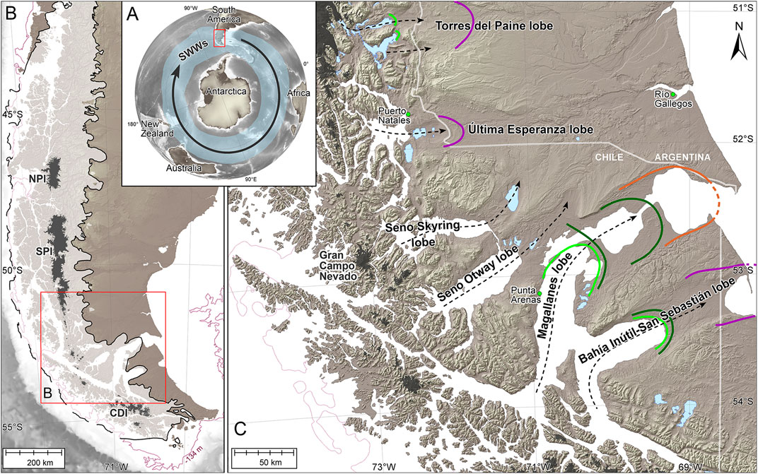
FIGURE 1. Location Map. (A). Location of Patagonia and the Southern Westerly Winds belt. (B). Extension of the Patagonian Ice Sheet during the LGM at 25 ka (pale grey shading, PATICE, Davies et al., 2020). Modern ice is shown by dark grey shading; NPI: Northern Patagonian Icefield, SPI: Southern Patagonian Icefield, CDI: Cordillera de Darwin Icefield. Bathymetric contour of -134 m indicates approximate fall in eustatic sea level during the LGM (Lambeck et al., 2014). (C). Location of Seno Skyring ice lobe in Southernmost Patagonia and adjacent ice lobes. Coloured arcs correspond to the age of dated moraine belts from the last glacial cycle: orange corresponds to MIS4, purple to MIS 3 and green to MIS 2 (Darvill et al., 2015; García et al., 2018; Peltier et al., 2021). Black dashed lines are hypothesised flow lines of major outlet lobes. Background image is a Copernicus DEM (30 m resolution).

2 General Setting and Study Area

2.1 Southern Patagonian Ice Sheet Setting

During the last glacial cycle in Patagonia, the PIS developed continuously along the Andean Cordillera from 38° to 55°S (Figure 1B), extending for about 2000 km (Glasser and Jansson, 2008; Rabassa, 2008; Davies et al., 2020). In southernmost Patagonia, the PIS extended to the west through tidewater-terminating outlets, calving into the Pacific Ocean. To the east, the outlets extended for 10–100 s of km across the Patagonian steppe (Figure 1C). The bed topography in this area is slightly unusual in the way the ice occupied reverse-bed slopes whose gradient varied between lobes (Kaplan et al., 2009; Anderson et al., 2012). The eastern area contains the best-preserved records of glacial geomorphology in the region as a result of its dry conditions and relatively stable tectonic context with no major uplift (Clapperton, 1993).

The climate in Patagonia is strongly influenced by SWWs, which impact the position of the Sub Tropical and Sub Antarctic Fronts. The SWWs are directly linked with precipitation (Garreaud et al., 2013), and their core is today located between ∼50–55°S (Lamy et al., 2010). During the winter months the SWWs’ core expands northwards and during the summer it contracts southwards, in response to seasonal changes in the Antarctic sea ice extent (Garreaud et al., 2013). The precipitation in western Patagonia ranges between 5,000–10,000 mm/year, decreasing abruptly towards the east to less than 300 mm/year (Garreaud, 2009), due to the orographic effect produced by the Andean Cordillera. This rain shadow effect strongly affects the vegetation in the area. Magellanic Moorland and evergreen forest are dominant in the west, and a few tens of kilometres east from the Andes Cordillera, the vegetation sharply changes to Patagonian steppe (Tuhkanen et al., 1989-1990).

We focus here on the southernmost part of the PIS, from the former lobe in Torres del Paine–derived from the southernmost tip of the present-day Southern Patagonia Icefield–south to the former Bahía Inútil-San Sebastián lobe that extended across Tierra del Fuego (Figure 1C). This region incorporates a range of different topographic settings from former outlets that terminated close to the mountains (10 s of km length) with a steep slope (such as Torres del Paine, and Última Esperanza), to low-gradient outlets terminations that extended 100 s of km east across the low elevation areas of Patagonia, such as Magallanes, and Bahía Inútil-San Sebastián lobes (Benn and Clapperton, 2000b).

2.2 Study Area and Previous Work

The Seno Skyring ice lobe originated at Gran Campo Nevado ice cap (52°40′S), a remnant of the continuous extension of the PIS along the Austral Andes, which has altitudes up to ∼1,500 m a.s.l. From there, the ice lobe extended to the east of the Andes (Kilian et al., 2007), sculpting deep valleys that today form the fjord of Seno Skyring (Figure 1C). Caldenius (1932) was the first to identify four moraine systems deposited east of Seno Skyring (Figure 2); we follow Caldenius’ nomenclature for the moraine systems. After Caldenius’ (1932) map, Meglioli (1992), Lovell et al. (2012), and Darvill et al. (2014) improved the glacial geomorphological mapping at a regional scale. Later studies suggested that the two inner moraine systems, Laguna Blanca (LB) and Río Verde (RV)—older and younger respectively—were formed during the last glacial cycle, based on the outlet glacier’s relationship with neighbouring dated glacial lobes (Darvill et al., 2017; Davies et al., 2020). A proglacial lake formed during the retreat between these two moraine systems (Caldenius, 1932). It has been hypothesised that a partial proglacial drainage may have occurred in front of the receding Seno Otway and Magallanes lobes (Benn and Clapperton, 2000b; Lovell et al., 2012; Darvill et al., 2014). Dating of organic material in fjord cores, suggest that towards the end of the last glaciation the Seno Skyring ice lobe had retreated back and was confined to the proximity of the Gran Campo Nevado ice cap by 13.9 ± 0.3 cal. BP (Kilian et al., 2007; 2013). Until the study we present here, no detailed mapping and chronological control existed for the Skyring lobe.

FIGURE 2

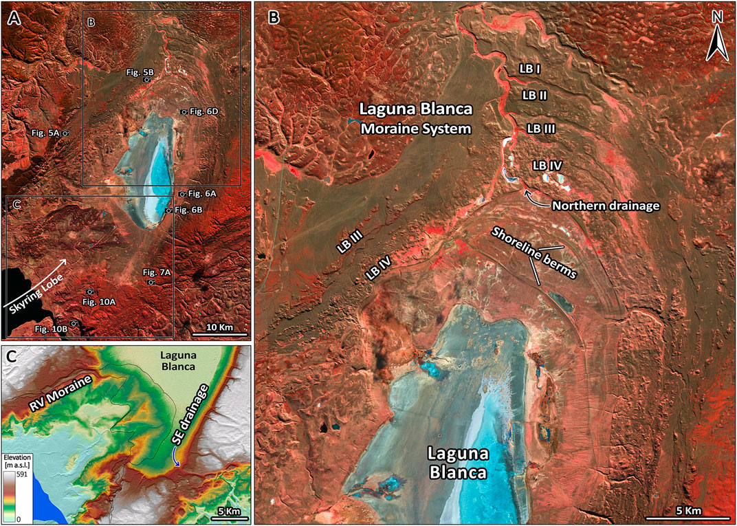
FIGURE 2. (A) Sentinel 2 (band combination 843) image of the Seno Skyring ice lobe area. Former ice flow of the Skyring lobe was directed from Seno Skyring north-east to the Río Verde (RV) and Laguna Blanca (LB) moraine systems. (B) Detailed image with focus on LB moraine system, showing its four different moraine belts, from older to younger LB I, LB II, LB III and LB IV respectively. Former shoreline berms and a northern drainage spillway of the palaeo Laguna Blanca are indicated. (C) Hillshade and elevation colour ramp (SRTM) of the area around RV moraine system, black lines indicate the RV moraine extension. The south-eastern drainage spillway of the palaeo Laguna Blanca is marked. Note that the altitude of this drainage spillway is higher than the central (front) parts of the RV moraine, implying an ice dam must have been present.

3 Methods

We undertook detailed geomorphological mapping and used the mapping to underpin the dating of key landforms to target glacial and deglacial events using cosmogenic ¹⁰Be surface exposure dating, a ¹⁰Be depth profile, optically stimulated luminescence (OSL) and radiocarbon dating methods. For ¹⁰Be cosmogenic measurements, we took samples of boulders on moraines, cobbles on major outwash plains and palaeo-shoreline berms, and measured ¹⁰Be concentrations to determine exposure histories. We also sampled one depth profile to determine the age of an outwash deposit using ¹⁰Be. These approaches have been widely used in semi-arid regions of eastern Patagonia (e.g., Kaplan et al., 2004; Hein et al., 2010; Darvill et al., 2015; García et al., 2018; Mendelová et al., 2020). Furthermore, we collected lacustrine sediment and bog samples to date with OSL and radiocarbon, respectively.

3.1 Geomorphological Mapping

The glacial geomorphologic map was compiled from stereoscopic analysis of aerial photographs, satellite images, and digital elevation models (Supplementary Table S1; extended methods). The geomorphological interpretations were field-checked over the course of several weeks of fieldwork campaigns in 2018 and 2019. Mapping of former shorelines was supported by hand-held GPS measurement transects up to 35 km along the different terrace levels. The map was prepared in ArcMap 10.7.1 (Figure 3).

FIGURE 3

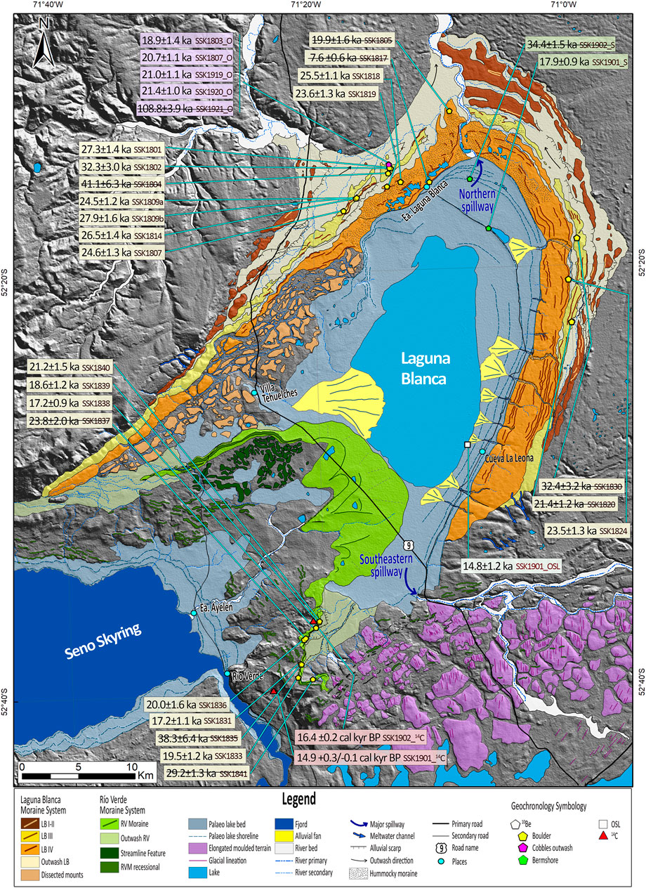
FIGURE 3. Geomorphological map of Skyring ice lobe area. Sample locations of the cosmogenic, OSL, and radiocarbon dates are indicated. Background is a hillshade from SRTM showing the topography. Dates treated as outliers are shown crossed-out, see text for discussion.

3.2 ¹⁰Be Dating

3.2.1 ¹⁰Be Exposure Age Sampling

3.2.1.1 Moraines

Timing of former glacial margins were constrained through two different approaches. The first method was by the sampling of moraine boulders along the different ridges. At the Seno Skyring lobe, we sampled along LB and RV moraine systems (Figures 2, 3). For LB moraines, we collected samples from multiple crests located in LB moraine III and IV. For the RV Moraine, we collected samples at the outer crest of the southeast lateral moraine. The boulder and the sampling process followed the methods of Gosse and Phillips (2001). Sampled boulders were primarily granitoid (n = 17), with some quartzites (n = 4) and one quartz arenite, all embedded in stable positions on or near moraine crests. Heyman et al. (2016) suggested that taller boulders yield more consistent results, since their tops are less likely to have suffered exhumation. We sampled boulders that were >1 m high where possible (32%), but otherwise sampled smaller boulders with ranges of 60–99 cm (45%) and 45–59 cm (23%) high (Table 1). For the lower relief boulders, we were careful in avoiding boulders with signs of exhumation by a visual assessment of the moraine degradation. We sampled top surfaces using nail gun cartridges and/or a hammer and chisel, avoiding erosional signs such as fresh edges, spalling or fracturing. Boulder SSK1809, had prominent quartz veins, with mean relief of 20 mm above the rest of the rock surface. We took two different samples from this boulder: SSK1809a from the boulder matrix and SSK1809b from the quartz vein (Figures 4K,L). We interpret the ¹⁰Be on moraine boulders as minimum ages for the moraine construction and associated glacial advance.

TABLE 1

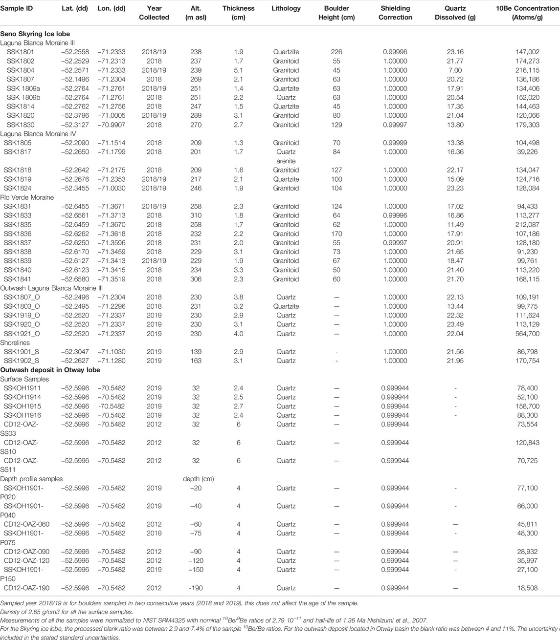
TABLE 1. Sample details and ¹⁰Be concentrations from Skyring ice lobe and the outwash deposit located in Otway basin, associated with the southeastern Laguna Blanca spillway. The samples are grouped by landform.

FIGURE 4

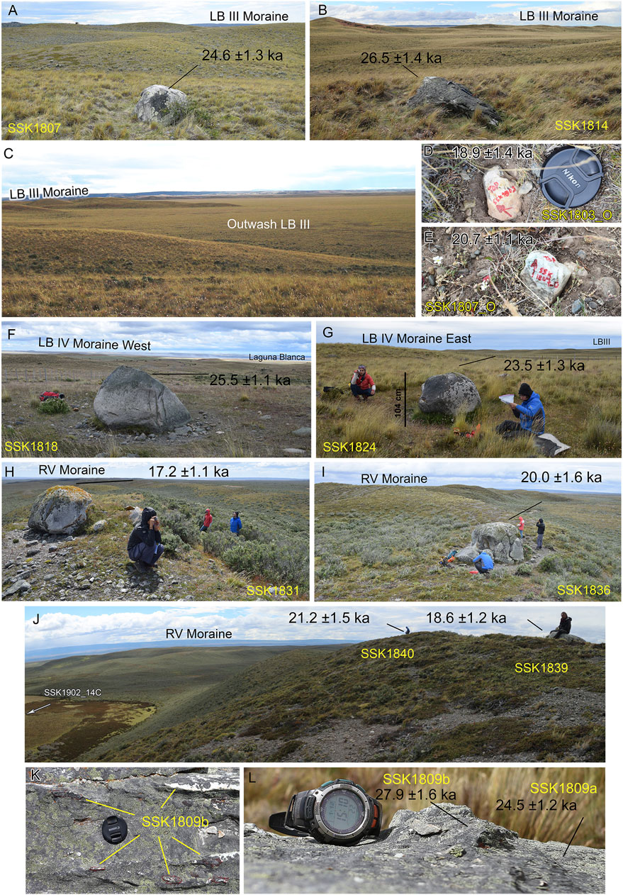
FIGURE 4. Examples of moraine boulder samples and outwash cobbles collected. (A,B) Moraine boulders from LB III. (C) LB III outwash. (D,E) Cobbles collected from LB III outwash. (F,G) Laguna Blanca IV. (H–J) RV moraine. (K,L) Sample SSK1809 showing the sampled quartz vein and sampled boulder surface.

3.2.1.2 Outwash Plains Associated to Moraine Margins

The second approach to dating glacial margins was to sample five quartz-rich cobbles embedded in the surface of an outwash plain grading from the LB Moraine III (Figures 4C–E). This follows the methodology of Hein et al. (2010; 2011), where outwash plain deposition is assumed to be broadly synchronous with associated moraine formation (Darvill et al., 2015; Mendelová et al., 2020). On imagery and in the field, the outwash plain was linked continuously to the external ridge of LB Moraine III, but the sample collection was located far enough (∼100 m) from the moraine to avoid subsequent downslope deposition. The age of these cobbles provide the minimum age of the outwash deposition.

3.2.1.3 Palaeo Lake Levels

We sampled two distinctive former shorelines around Laguna Blanca for cosmogenic ¹⁰Be exposure dating. These shorelines are located at the inner part of the frontal LB Moraine (Figures 2, 3) and we assume the source of material corresponds to till eroded by the lake. For each shoreline, we took one sample composed of an amalgamation of ∼30 cobbles and large quartz pebbles (Mendelová et al., 2020). We collected the samples on flat top surfaces of wide beach ridges; these berm ridges are large-scale features and surrounded by relatively flat relief within a 2 km radius, so we are confident no material has been deposited on the surfaces since they were deposited. The age resulting from the amalgamated samples indicates a minimum age for the shoreline berm formation.

3.2.2 ¹⁰Be Depth Profile From an Outwash Located on the Otway Basin

Previous geomorphological mapping reconstructions (Lovell et al., 2011; Darvill et al., 2014), and our own work link an outwash terrace in the area formerly occupied by the Seno Otway lobe to a drainage event south-eastward from a palaeo Laguna Blanca proglacial lake associated with the Seno Skyring lobe. Dating this deposit should constrain the timing of lake drainage and provide limiting ages for glacier retreat. We adopted two approaches to dating methods on this deposit.

Firstly, we collected surface samples to obtain exposure ages. From the surface of the outwash terrace, we sampled seven mono-mineral quartz cobbles (Table 1).

Secondly, we samples a depth profile in the outwash and modelled nuclide concentrations using Monte Carlo simulations. This approach can be used to calculate the most likely age, erosion rate, and nuclide inheritance ranges of a deposit (Hidy et al., 2010; Rodés et al., 2011; Darvill et al., 2015). The outwash deposit is formed by unconsolidated material composed mainly of pebbles and coarse sand with matrix-supported, grading to different percentages along it. The sediments of the outwash terrace appear to have been deposited continuously, and the surface does not show clear evidence of post-depositional reworking, cryoturbation or bioturbation (e.g., surface meltwater channels are preserved), making it suitable for dating with this approach (Hein et al., 2009, 2011; Darvill et al., 2015; Cogez et al., 2018; García et al., 2021). We collected eight samples from this profile from 20 to 190 cm below soil depth through a section of a modern anthropogenic road-gravel quarry in the outwash at this location (Table 1). Depth profile samples were amalgams of quartz pebbles and sand from ∼4 cm thick layers at each depth. Samples were collected in two stages from the same sequence, in 2012 and 2019, following the methodology of Darvill et al. (2015). Soil development on the outwash surface is poor, with an average thickness of ∼15 cm. Because the stratigraphy is not homogeneous, we estimated the density for each stratigraphic layer and accounted for layer thickness. We estimated the percentage of clasts bigger than sand for each layer, to which we allocated a density of 2.7 g/cm³. For the rest of the layer, the sand and porosity, we gave a density of 2.7 g/cm³ and 0, respectively. The porosity values for sand and gravel were taken from the data for unconsolidated materials of Manger (1963), using the porosity range for each layer. We calculated the density proportional to the amount of each material (Hancock et al., 1999), yielding a density range of 2.1–2.3 g/cm³.

3.2.3 ¹⁰Be Laboratory Process

The boulders and surface cobble samples were prepared in a combination of the cosmogenic labs. The quartz isolation for moraine boulders and shorelines was performed at Universidad Católica in Santiago, Chile and Edinburgh University, United Kingdom. We obtained clean quartz using acid etching techniques following Hein et al. (2009) methods. The ¹⁰Be/⁹Be measurements were carried out at the Köln AMS, Germany (Dewald et al., 2013), normalized to the revised standard values reported by Nishiizumi et al. (2007). For methodological details refer to supplementary material. Final ¹⁰Be concentrations and uncertainties are reported in Table 1.

The samples from the outwash terrace located on the Otway lobe, were entirely prepared at Scottish Universities Environmental Research Centre as part of the United Kingdom NERC National Environmental Isotope Facility. The surface samples were treated individually, while the samples from the depth profile were treated as amalgams. For the details of the sampling process from quartz isolation and purification, BeO separation, and AMS analysis, see supplementary material; extended methods. The ¹⁰Be concentration, uncertainties, and samples details are given in Table 1.

3.2.4 ¹⁰Be Exposure Age Calculation

The ages were determined with the online calculator, formerly known as the CRONUS-Earth online calculators, version 3 (Balco et al., 2008). We applied the Patagonian ¹⁰Be production rate calculated from Lago Argentino (Kaplan et al., 2011). We use a general quartz density of 2.65 g/cm³ for all the samples. The topographic shielding factor was negligible, with values between 0.999–1. We calculated the shielding by measuring the horizon geometry every 15° with a hand clinometer, then we converted these data to the shielding factors in the online calculator formerly known as CRONUS-Earth (https://hess.ess.washington.edu). For calculation and discussion of results in context with the other results in the region, we follow previous workers in assuming zero erosion and no correction for vegetation or snow cover of the boulders. However, from sample SSK1809b, we can calculate an erosion rate and we briefly discuss its implications below. For the age calculations, we used the Lm scaling scheme (Lal, 1991; Stone, 2000). Selecting a different scaling scheme would not significantly affect our conclusions. The sample characteristics and ¹⁰Be data are given in Table 1. For the moraine ages, we present the weighted mean of the boulders with one weighted standard deviation as uncertainty. To identify outliers in each moraine group of samples, we use chi-square $\left({\text{χ}}_{\text{R}}^2\right)$ statistics. This method rejects samples outside the 2σ envelope, considering the number of samples (Wendt and Carl, 1991). If ${\text{χ}}_{\text{R}}^2$ < κ, the samples fall within the 2σ (Spencer et al., 2017). These calculations are made using the web calculator IceTea (Jones et al., 2019; http://ice-tea.org) when plotting a group of samples from a single moraine.

For the age comparisons with other ice lobes on the discussions, we recalculated previously published ages to Lm scaling scheme with the Patagonian production rate (Kaplan et al., 2011), with no correction for erosion, and no correction for snow or vegetation cover, to allow for direct comparisons between datasets.

3.2.5 ¹⁰Be Depth Profile and Surface Ages From Outwash Deposit in Otway Basin Calculation

For the depth profile and surface samples, we applied the ¹⁰Be production rate from Kaplan et al. (2011), calculated in the online calculators formerly known as the CRONUS-Earth online calculators v.3 (Balco et al., 2008) using the Lm scaling scheme (Lal, 1991; Stone, 2000). Thus, we used production rates of 4.3644, 0.01803, 0.03818 atoms/g/year and attenuation lengths of 160, 5,850, 500 g/cm² for spallation and fast and negative muons, respectively. For surface samples, we assumed zero erosion and densities of 2.65 g/cm³.

To model the depth profile age we use the approach from Rodés et al. (2011) and we fitted the depth profile model to our data using the same combine surface exposure-burial MATLAB scripts as described in Rodés et al. (2014). The model requires input ranges for the deposit’s possible ranges of density, age, and erosion rate. We constrained the density according to our calculations, and we used a range between 2.1 and 2.3 g/cm³. A sensitivity test with a broader density range of 1–3 g/cm³, showed little effect on age, erosion rate and inheritance and so use of a smaller density range is justified. For the possible age range, we are confident based on chronology of other ice lobes (Darvill et al., 2015; García et al., 2018; Peltier et al., 2021), that in the region the ice filled the Otway basin during the last glacial cycle. Nevertheless, we are ultra-cautious and use an age range of 0–1.1 Ma, where the maximum age corresponds to the greatest Patagonian Glaciation (Meglioli, 1992; Singer et al., 2004). We did not constrain the erosion rate of the deposit since we did not have independent information to do so. For each sample depth, we applied a conservative ±2 cm measurement error, which corresponds to the 4 cm sampling strip.

The Monte Carlo method utilises different solutions that best fit the given variables, that include depth profile sample ¹⁰Be concentrations, density, age-range, and erosion rate of the deposit. The modelling shows all the possibilities that adjust with the given variables within a one sigma solution. We performed 50,000 models, and we obtained 3,771 possible results within one sigma of the data. Because this method is a probabilistic approach, it is possible to have different solutions that fit the given inputs. Thus, the model results are given in ranges, where different answers can be correct, especially if the input data are broad or unconstrained. Nevertheless, the model suggests the most likely data.

3.3 Optically Stimulated Luminescence

We used OSL dating to determine the age of raised lacustrine deposits around Laguna Blanca’s margins. The OSL sample was taken from a 30 cm-thick sand layer, with medium sand grain size embedded within a lacustrine profile, located at the lowest palaeo lake terrace (T6). These sediments overlie glaciolacustrine sediments (with dropstones) but the context and sedimentology of the sampled layer corresponds to an alluvial fan deposit that is interfingered with lacustrine sediments and thus this age provide the timing of a higher lake levels previously to the erosion of level T6. Samples for luminescence dating were collected in opaque tubes hammered into the section and the ends sealed. These were prepared for analysis under subdued lighting conditions following the methodology of Smedley et al. (2016) Supplementary material.

3.4 Radiocarbon

We use radiocarbon dating to constrain the peat initiation of two different sites located within and inboard of the innermost RV moraines, using a Wright Piston Corer. The samples were cleaned by wet sieving to remove any potential coal present. Cleaned samples were sent to the DirectAMS radiocarbon dating service for final preparation and measurement. We calibrated the ages to calendar years in CALIB 8.2 program (calib.org; Stuiver et al., 2021) using the SHcal20 curve (Hogg et al., 2020). We report the calibrated ages using the 2-sigma calibrated range.

4 Results

4.1 Geomorphology

The geomorphological relationships of the landscape observations are shown in the geomorphological map (Figure 3), and the criteria used to map them are explained in Supplementary Table S3 (extended results).

4.1.1 Laguna Blanca Moraine System

The Laguna Blanca moraine system comprises at least four distinctive moraine belts separated by clear outwash plains; they are LB I, LB II, LB III and LB IV from oldest to youngest (Figure 2B). They are located in an arcuate arrangement around Laguna Blanca. In the frontal section, 10 km separates LB I from LB IV. A major meltwater spillway of a palaeo Laguna Blanca that was bigger than the present, cuts through this moraine system from the northern point of the Laguna Blanca former basin. We use this outlet to divide the glacial margins into East and West. On the eastern side of the system, the moraines are confined to the high ground that separates the basins of the former Seno Skyring and Seno Otway glacier lobes. On the west, the moraines are more widely spaced than on the eastern side. The outwash plains are narrower at the lateral parts, and they widen—up to 2 km wide in some places—as they get closer to the front of the lobe. The landform preservation decreases towards the outer moraines due to subsequent meltwater erosion, partial, overriding of the older moraines by younger glacial advances and by moraine ridge degradation through time. The outer LB moraine (LB I and LB II) relief is restricted to discontinuous ridges that we link together as a margin due to continuity of associated outwash plains along an arcuate pattern. Nevertheless, these moraines have good local preservation in the northeast area of the ice lobe, with moraine belts ranging between 1 and 2 km wide. On the other hand, the two inner moraine belts (LB III and LB IV) are preserved almost continuously enclosing Laguna Blanca. Despite the relatively poor preservation of the outer belts, all four LB belts expose similar morphostratigraphic characteristics. They have relief in general between 10–15 m high, but in some places, they can be up to 20 m, and their distal slopes are about 7° and their proximal 9° (Figure 4A-G). To the east, the large dimension of the inner moraine belt (LB IV) stands out, where they are up to 4 km wide in some areas and have close to 40 km of continuous lateral extension. There, the LB IV has close to 10 parallel nested ridges. The morphology is very different from the central and western area where LB III and IV are formed by a group of hills or short ridges with little structure. Hummocky relief is common in the central area, with significant intermorainic depressions. The western area is pervasively affected by meltwater erosion. Several meltwater channels cut the moraines and the outwash plains with alignments subparallel to the moraine ridges. The meltwater channels can be traced upstream to the Seno Skyring ice lobe’s southwest margin. Exposed sections along the moraine belts were scarce. Nevertheless, we identified two lacustrine sediment slabs within sections from LB I and LB IV (Figure 5). These slabs were located in near-horizontal positions with regard to the sediment’s lamination. These sediments have pervasive climbing ripple cross-lamination structure and exhibit slight brittle deformation and are overlain by till.

FIGURE 5

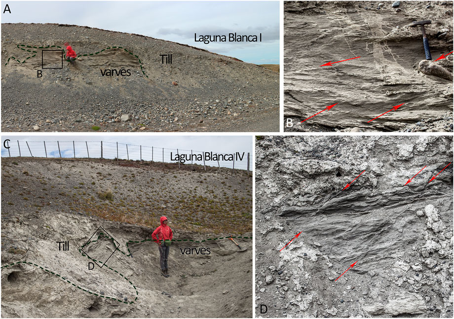
FIGURE 5. Cut profile from LB moraines, showing lacustrine sediments overlain by till. (A,B). LB I. (C,D). LB IV. The sediments have climbing ripple cross-lamination structure. The sediments show evidence of brittle deformation indicated by red arrows.

4.1.2 Laguna Blanca Palaeo Lake

On the inboard margins of the LB moraines, we identified six distinctive raised shorelines corresponding to formerly higher levels of the palaeo Laguna Blanca (Figure 6). They are located on the western and eastern sides, named T1 to T6 from older (highest) to younger (lowest), respectively and the elevations of the terraces are illustrated in Figure 6E. T1 and T2, were only observed to the north, and they are just represented as terraces. T3 to T6 have a good lateral continuity to the south, their frontal part is in the forms of shoreline berms while the lateral parts are terraces, interpreted as cut-wave terraces, and they are better preserved on the east side (Figure 3). The different levels of the upper shorelines are separated by clear scarps, with the best example being the scarp between T3 and T4 with close to 10 m of relief. In the lower terraces, these scarps are less obvious, and we simply observe a change in the slope of the terraces. Furthermore, on the east side, several alluvial fans cover the terraces with material derived from erosion of LB moraines located upslope. Our GPS surveys show that the terraces dip at low angles down towards the NNE (i.e., down-glacier direction). The greatest slopes are found on the highest shorelines, and they decrease to nearly horizontal angles towards the lowest (Figure 6E).

FIGURE 6

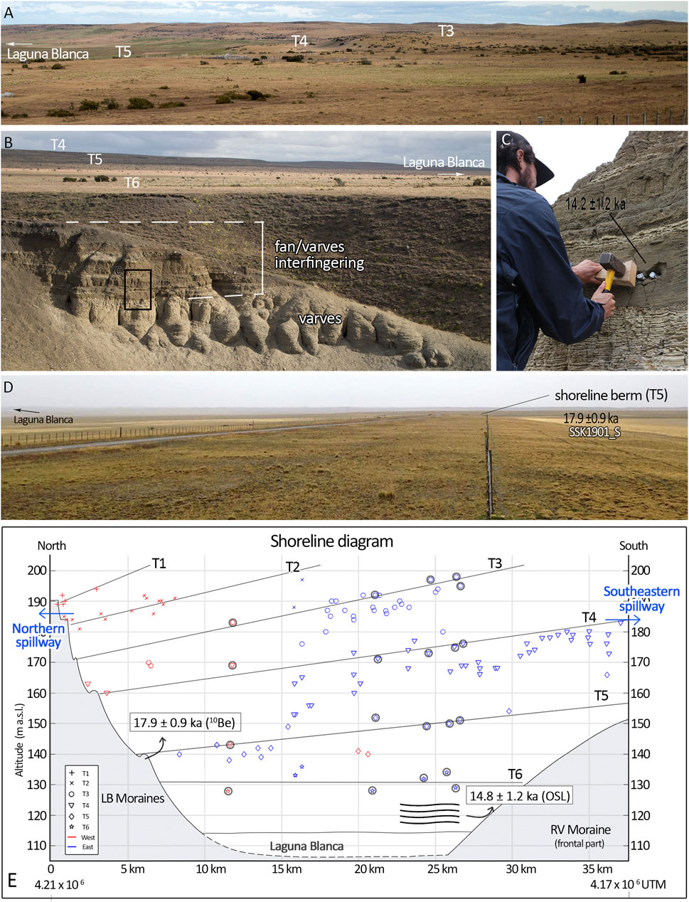
FIGURE 6. Palaeo shorelines of Laguna Blanca. (A) Three terrace levels seen at the eastern side of Laguna Blanca. (B) Incision of the lowest terrace, T6, exposes glaciolacustrine and alluvial fan sediments. (C) OSL sample from a sand layer of the lacustrine profile (see panel b for location). (D) Palaeo shoreline berm located at the north part of Laguna Blanca, this berm is related to T5. (E) Shoreline Diagram of the former levels of Laguna Blanca. The symbols surrounded by a black circle correspond to the measurements done on the scarp base. The locations are marked of a ¹⁰Be age of the shoreline berm on T5, and an OSL sample of a subaqueous alluvial fan taken from araised shoreline forming part of terrace T6. Data from west (red) and east (blue) are differentiated. The elevations and positions of the northern and south-eastern drainage spillways are marked. See legend for shoreline/terrace numbering.

We mapped two different former spillways for deglacial palaeolake Laguna Blanca. One, located in the north, cuts the frontal area of LB moraines, has an altitude ∼185 m a.s.l, and is about 150 m wide. The northern spillway was active during the lake levels of T1 and T2 (Figure 6E). Once the lake level lowered from T2, this spillway was abandoned. The second spillway is located in the southeast of the Laguna Blanca basin and cuts through soft bedrock in a series of anastomosing channels towards the Otway ice lobe (Figure 3; Figure 7A). The southeastern spillway has an altitude ∼183 m a.s.l, and is about 300 m wide. This spillway drains east, where it divides into several minor channels, braiding for about 30 km before reaching the Otway basin (Figure 7F). Downstream of the spillway there are broad outwash terraces aligned in a west-east direction and which wrap around discontinuous older moraine ridges in the Otway basin (Lovell et al., 2012; Darvill et al., 2014; Figure 7E,F). The morphostratigraphic relationship between the spillway and shorelines show that this spillway was active when the lake level was at T4. We speculate that the major size of the spillway may be due to it being the route for large volumes of water during a relatively rapid partial drainage of the lake as it lowered from T3 to T4 (Figure 6E). After the lake level decreased from T4, this second spillway also became abandoned. T5 and T6 formed subsequently when the lake did not have any apparent spillway.

FIGURE 7

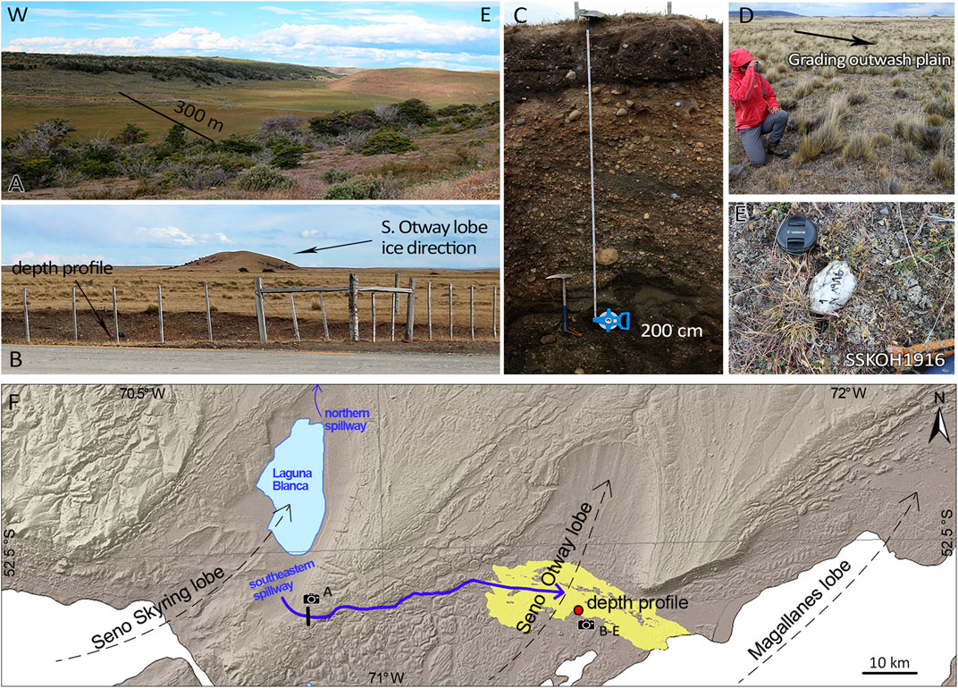
FIGURE 7. Geomorphological record of drainage of Laguna Blanca through the southeastern spillway. (A) Southeastern drainage spillway viewed from the south. (B) Moraines of the Otway lobe surrounded and partly-buried by a later outwash deposit on both distal and proximal sides. (C) Depth profile of the outwash that buries the Otway moraines. (D–E) Cobbles sampled for cosmogenic analysis on the surface of the outwash. (F) Map showing the mapped drainage route from the southeastern spillway of the Seno Skyring basin towards the Otway lobe basin.

In T6, several incisions cut the distal part of the terrace, exposing large sediment sections (52.4°S; 71.1°W), at the eastern part of the Laguna Blanca (Figure 6B). These sections show a consistent stratigraphy composed at the bottom by at least 6 m of varves composed of clay and silt intercalation, with mm-scale horizontal lamination. Additionally, angular and rounded dropstones are embedded within the varves. On top of this unit, dropstone-free laminae are interfingered with sand and gravel with thicknesses ranging from 10 to 70 cm (Supplementary Figure S1, extended results). The sand and gravel layers have wedge-shaped beds becoming thinner towards Laguna Blanca and their base contact is always erosive, while in the varve layers the wedge shapes become thinner in the opposite direction. For OSL dating, we sampled a coarse sand layer located immediately on top of the 6 m of clay/silt unit (Figure 6C).

4.1.3 Río Verde Moraine System

The younger moraine system RV is located about 30 km inboard of the LB moraine system. It consists of one prominent terminal moraine and numerous recessional smaller moraines. The morphology of the terminal moraine has a sharp change in morphology at an elevation of 160 m a.s.l. between the lateral and frontal parts. The higher parts of this moraine system, located between 160and 310 m a.s.l., are generally higher relief and sharper-crested than the LB moraines. In the higher, lateral sections, the relief of the ridges range from 30 to 35 m, and their distal and proximal slopes are close to 16° and 20°, respectively (Figures 4H–J). The frontal (central) section of this terminal moraine is at a lower elevation (between 120–160 m a.s.l.) with much broader, flat and rounded ridge crests. It is composed of four coalescent ridges in an arcuate shape (Figure 2C). This frontal feature can be mapped on imagery but is almost imperceptible in the field; its relief of about 20 m was unnoticeable on the ground due to its width of ∼10 km.

Streamlined landforms are visible on the proximal part of the northwest RV moraine. They are low flat-topped hills with rounded limits, elongated concordant with the ice direction. We mapped discontinuous moraine patches about 8 km inboard from the outer RV belt. Further inboard of these recessional moraines are at least four distinctive shorelines terraces marked by the presence of sub-vertical scarps. These terraces step down in height from 60 m a.s.l. to the present shoreline of Seno Skyring to the west.

4.2 Geochronology

4.2.1 ¹⁰Be Exposure Ages

4.2.1.1 Laguna Blanca Moraine System

The presence of boulders on the LB moraines is extremely scarce. Nevertheless, we processed thirteen boulders for ¹⁰Be exposure cosmogenic dating from this moraine system. We present data from the moraine LB III and LB IV in this system (Table 2; Figure 4). Additionally, we processed four surface cobbles located in the outwash plain apparently grading from LB III (Figures 4C–E).

TABLE 2

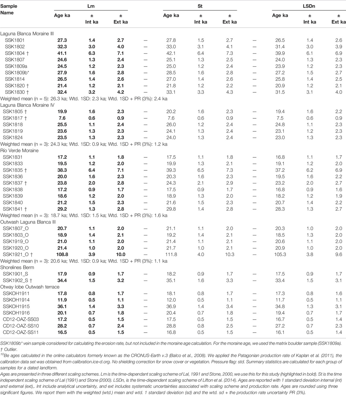
TABLE 2. ¹⁰Be ages for the study area, assuming 0 erosion rate.

On LB III, we collected eight boulder samples, six from the western lateral part and two from the eastern part. Even though these moraines do not have continuous parallel ridges, the samples SSK1801, SSK1802 and SSK1820 were collected at the outer most part. SSK1807, SSK1809a and SSK1814 were at the intermediate position, SSK1804 and SSK1830 were taken at the moraine’s inner part. On LB III, three samples fall outside the 2σ envelope, therefore they would be considered outliers. Finally, for LB III, five boulders yielded ages ranging from 32.4 to 25.0 ka with a weighted mean of 26.3 ± 2.3 ka (Figure 8A).

FIGURE 8

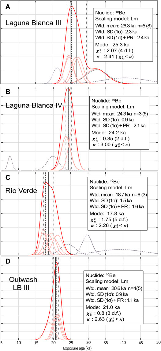
FIGURE 8. Probability density functions (“camel plots”) of the ages for moraines and outwash of the former Skyring ice lobe. All ages are calculated with the Patagonian production rate from Lago Argentino (Kaplan et al., 2011) and considering zero erosion. (A) Laguna Blanca III. (B) Laguna Blanca IV. (C) Río Verde moraine. (D) Outwash Laguna Blanca III. n corresponds to the number of samples used to calculate the weighted ages. Bracket numbers are all the samples processed, including outliers. The diagrams were plotted using IceTea (Jones et al., 2019), where the mode (black dashed line), weighted mean (solid black line) and weighted standard deviation (SD; black dotted lines) of the dataset are shown. The application also calculates the reduced chi-squared (${\text{χ}}_{\text{R}}^2$) and the associated criterion (κ). The outliers are shown as grey dashed lines; they were calculated following reduced chi-squared statistics.

On LB IV moraine, we sampled five boulders. Four of them (SSK1805, SSK1818, SKK1819, SSK1924) were located in the outer part of the moraine, and one (SSK1817) at the inner part. Two boulder ages were rejected as outliers, including the boulder located at the inner part of the moraine. The three samples yielded ages ranging from 25.5 to 23.5 ka, and a weighted mean of 24.3 ± 0.9 ka (Figure 8B).

We collected five cobbles from LB III outwash plain. One sample (SSK1921_O) was rejected as an outlier with an age of 108.8 ± 3.9 ka. The remaining four cobbles yielded ages ranging from 21.4 to 18.9 ka, with a weighted mean of 20.6 ± 0.9 ka (Figure 8D).

4.2.1.2 Río Verde Moraine System

In the RV moraine system, there were more abundant moraine boulders than in the LB moraines. We sampled nine boulders on the outer ridge of the eastern lateral section of the RV terminal moraine between 230–310 m a.s.l., above any potential palaoelake level (Figures 3, 4). Three samples (SSK1835, SSK1837, SSK1841) were rejected as outliers (Table 2). The remaining six (SSK1831, SSK1833, SSK1836, SSK1838, SSK1839, SSK1840) samples yielded ages ranging from 21.2 to 17.2 ka with a weighted mean of 18.7 ± 1.5 ka (Figure 8C).

4.2.1.3 Boulder Erosion Rate

We calculated the erosion rate for one boulder (SSK1809) in the Skyring area by sampling quartz veins standing out by approximately 20 mm from the upper rock surface (Figures 4K,L). The vein sample, SSK1809b, has an age of 27.9 ± 1.6 ka. Assuming the quartz veins have experienced zero erosion, we calculated a linear-erosion rate of 0.72 ± 0.04 mm/kyr for this quartzite lithology. We assumed a zero erosion rate for the boulders (Table 2) because the erosion rate calculated was just performed on one boulder, which may not represent all the other boulder positions or lithologies. Moreover, the use of zero erosion allows us to compare to other studies in southern Patagonia, which also widely assume zero erosion. Nevertheless, to illustrate the effects of potential erosion, we additionally provide the boulder ages for only quartzite lithology, calculated using a 0.72 mm/kyr erosion rate (Supplementary Table S4, extended results). The age difference is minimal when applying this erosion rate for boulders with quartzite lithology. Boulders dated to about 30 ka increase in ∼600 years with the erosion rate correction, and boulders dated to about 20 ka increase by ∼200 years, which is within the analytical uncertainty. Note that the vein age was utilised just for the erosion rate calculation, and for the LB III moraine age calculation we used the boulder matrix sample (SSK1809a).

4.2.1.4 Laguna Blanca Palaeo Lake

We ¹⁰Be dated T4 and T5 palaeo-shoreline berms from palaeo Laguna Blanca. The sample SSK1902_S (T4) yielded exposure ages of 34.4 ± 1.6 and the sample SSK1901_S (T5), 17.9 ± 0.9 ka (Figure 3). We rejected the sample SSK1902_S since it is anomalously old compared to the LB moraines ages. The most likely explanation for the anomalously old age is that some cobbles sampled in T4 contained inherited ¹⁰Be from previous exposure histories. Moreover, the age of a cobble (SSK1921_O) on the LB III outwash plain, ∼88 kyr older than the rest of its group, supports the presence of material with inheritance in the area.

4.2.2 ¹⁰Be From Outwash Deposit in Otway Lobe: Surface Samples and Depth Profile

The seven surface samples from the outwash deposit yielded apparent ¹⁰Be exposure ages ranging between 11.9 and 36.1 ka (Table 2). Four of the seven samples range between 20.1 ± 0.7 and 16.5 ± 0.5 ka, with a weighted mean of 17.7 ± 1.3 ka. Due to the scattered age range, and potential for deflation or inflation of the sediment surface and possibility of inheritance (Hein et al., 2011), we treat these data as apparent ages (Figure 9G).

FIGURE 9

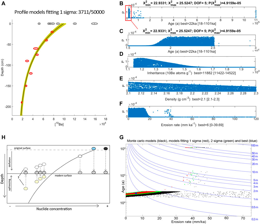
FIGURE 9. Depth profile model results from outwash deposit located in Otway ice lobe, associated with the southeastern Laguna Blanca spillway. (A) Plot of ¹⁰Be concentration of samples from the surface (grey circles) and depth profile (red circles), with their uncertainties as a function of depth. Green lines indicate the model results that fit within 1 sigma, the black line corresponds to the best fit model. (B–F) Probability density distributions of the different outputs of the model: age, inheritance, density, and erosion rate. (B) Shows the modelled ages plotted between 0–1,101 ka, whereas (C) shows the ages plotted between 15–30 ka. (G) Graphic showing relationship between age, erosion rate, and surface lowering. Red dots are model runs lying within 1-sigma of the data, green are those within 2-sigma, and black dots are other model runs. Model output shows 99.5% of data within 1-sigma lie within an age range of 18.6–25.1 ka, with a small component of well-fitting model runs that would require implausible (40–50 m) amounts of surface lowering. (H) Schematic cartoon to explain scattered age of the surface samples and reasons for their difference in age from the depth profile modelling. The older samples could have been exposed to the cosmogenic radiation from the outwash terrace formation (blue sample). If the samples have a component of inheritance from earlier exposure, then the age will be older than the terrace (black sample). A deflation of the outwash will expose samples that were initially buried, resulting in younger than the outwash age (white). Younger samples could also be raised to the surface due to inflation processes, such as upfreezing (see Hein et al. (2009), and Darvill et al. (2015) for further discussion).

The ¹⁰Be concentration of the depth profile samples reduces with depth (Figure 9A), consistent with a post-depositional nuclide production in a stable deposit without mixing sediments (Hein et al., 2009). Two exceptions are the samples located at 60 and 90 cm depth that could have mixed sediments or material with more ¹⁰Be inheritance concentration at the moment of deposition. It is also important to note that those two samples are the ones that have the largest uncertainty.

The ¹⁰Be depth profile modelling results demonstrate a modelled age range between 18–1,101 ka (Figure 9B) but with a most likely age between 19 and 25 ka (99.3% of solutions lie in this range; Figure 9C). For simplicity, we report this here as 22 ± 3 ka, whilst noting that this does not imply a normal distribution of ages and that different ages in this range may be equally likely (Rodés et al., 2011). The model yields a median inheritance estimate of between 11,422 and 14,522 ¹⁰Be atoms/g (Figure 9D). This indicates a minimum period of prior exposure longer than ∼2 kyr, if all the clasts came from the surface of the eroded deposit. Nevertheless, we know that the cosmogenic radiation decays with depth, and it is very likely that not all the clasts along the profile were located previously on the surface. Therefore, this exposure time is considered a minimum period. Moreover, as we cannot rule out that the eroded channels were active in more than one drainage event, the outwash deposition could have included material that was previously exposed, even in older glaciations. The model does not seem to be sensitive to variations in the density (Figure 9E), and this is also supported by the sensitivity test performed with broader parameters. For the erosion rate we obtained a range of 0–39.7 mm/ka (Figure 9F). The possible age solutions (0.7% of model runs) older than 22 ± 3 ka (Figure 9H) can be ruled out as requiring an unrealistic amount of surface lowering (40–50 m). Such high erosion rates are not likely in arid eastern Patagonia and our geomorphology observations show the outwash surface is well preserved with melt water channels with decimetre-scale scarps still visible on aerial photographs and imagery, and no signs of pervasive erosion.

We utilize the age modelled through the ¹⁰Be depth profile approach (22 ± 3 ka), as the most reliable constraint for this outwash deposit formation and we regard the slightly younger date from surface cobbles as only an apparent age of the deposit.

4.2.3 Optically Stimulated Luminescence and Radiocarbon

The OSL sample SSK1901_OSL yielded a deposition age of 14.8 ± 1.2 ka. This sample was collected from a sand layer exposed along the T6 terrace (Figures 6B,C).

We constrained the deglaciation by ¹⁴C dating of the glacial (inorganic) and peat sediment contact using two ¹⁴C samples from two bog sites within and inboard of the RV moraines (Figure 10). One site is a peatbog occupying an intermorainic depression just inside RV terminal moraine. At this site, we cored through peat for 1,080 cm, until we reach lacustrine sediments. The sample SSK1902_14C consisted of amalgamated macro plant fossils collected right above the sharp contact between the peat and the lake sediments. The 2σ calibrated age range is 16,236–16,571 cal year BP, for convenience from here on we express the age as c.16.4 cal kyr BP (Table 3). Furthermore, the sample site of SSK1901_14C is a bog in an abandoned meltwater channel located inboard and at a lower elevation. There, we cored 575 cm of continuous peat until we reached coarse inorganic sand. The ¹⁴C sample consisted of plant macrofossils obtained from just above the sharp contact between the inorganic sand and the overlying peat. The 2σ calibrated age range of the maximum probability is 14,781–15,143, from here on we express this age as c.14.9 cal kyr BP (Table 3). The cores from both sites showed sharp contact between inorganic sediments and the peat sedimentation. The type of sedimentology indicates a primary mire formation of peat initiation. This means that the peat originated on newly exposed waterlogged land (Ruppel et al., 2013; Quik et al., 2021). The abrupt nature of the contact suggests a deglaciation event (e.g., Hall et al., 2013; McCulloch et al., 2020).

FIGURE 10

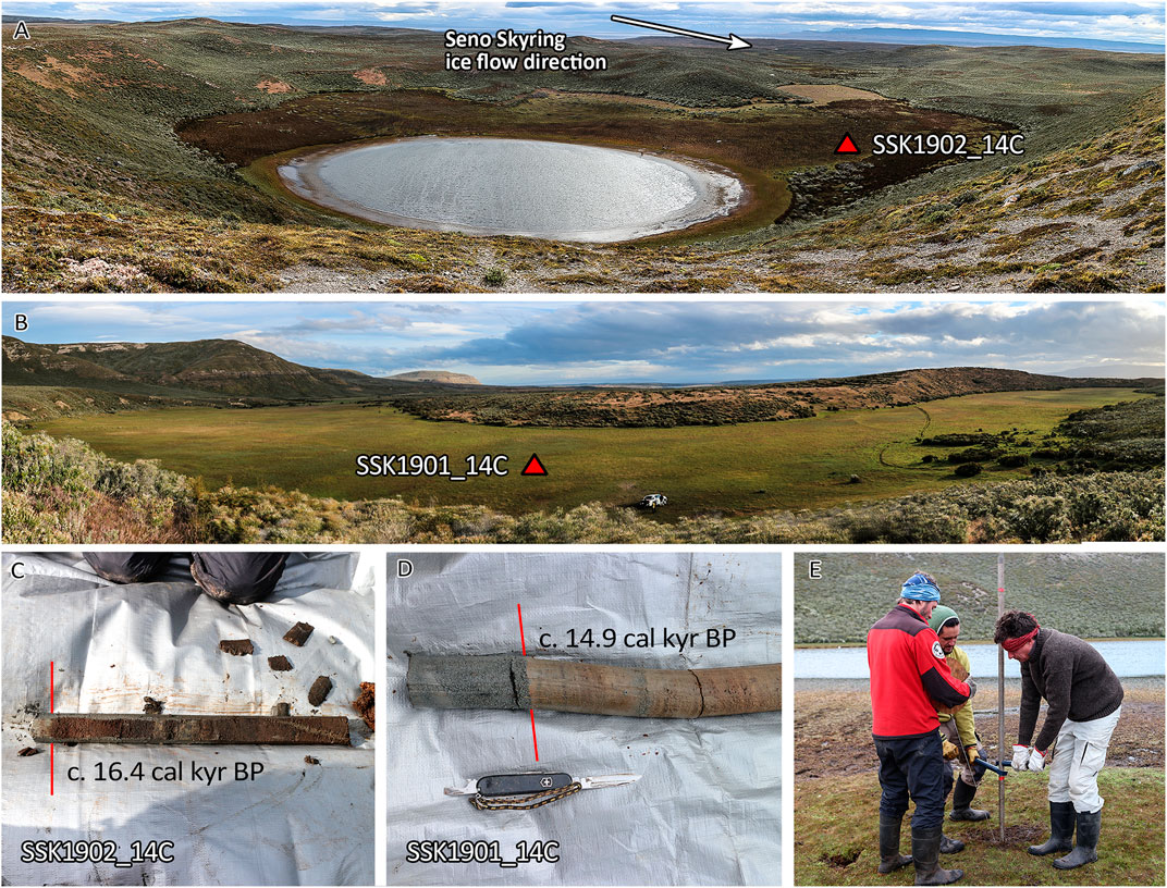
FIGURE 10. (A–B) Sample location for radiocarbon dating in peat bogs (red triangles). In (A), the core was taken close to the margin of a lake sitting on the proximal side of the terminal RV moraine. In (B), the core was taken from an abandoned meltwater channel. (C–D) Core samples from both sites, red lines indicate the contact between organic and inorganic materials, mud and sand sediment, respectively. (E) Wright piston corer being used to sample SSK190214C.

TABLE 3

TABLE 3. Radiocarbon sample details.

5 Discussion

5.1 Geomorphology and Sedimentology Interpretation

5.1.1 Laguna Blanca Moraines

We use our geomorphological mapping to compile a relative chronology of glacial advances and deglaciation, which we show in Figure 11, and for which we provide a geochronology in the following section.

FIGURE 11

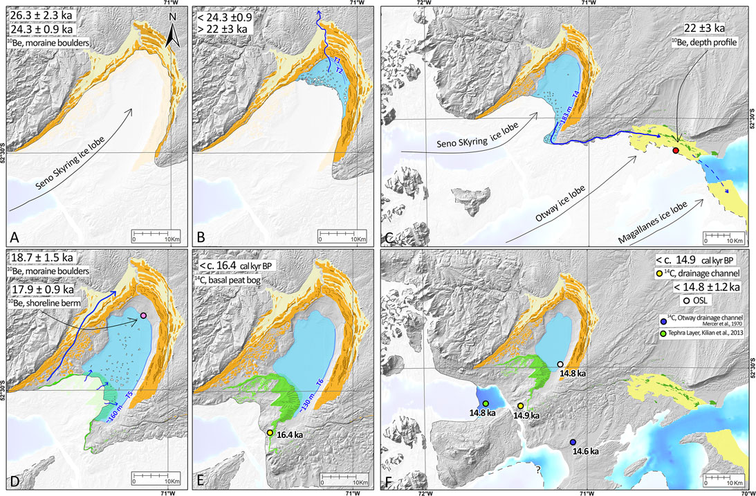
FIGURE 11. Evolution of the former Seno Skyring ice lobe. (A) Glacier position during the deposition of LB III and LB IV moraines. (B) Formation of the Laguna Blanca proglacial lake with a northern spillway. During this period, the northern spillway served as drainage for T1 and T2 lake levels. (C) Abrupt (partial) drainage of Laguna Blanca to the southeast reaching the Otway lobe region, lake level decreased rapidly from T3 to T4. (D) Glacier position during the deposition of RV moraine; the frontal parts formed sub-aqueously under the lake level T5. During this glacial advance/stillstand, the outwash from LB moraines was reactivated at 20.6 ka. (E) Minimum age of the glacier abandonment from RV moraine position. (F) The Seno Skyring and Otway lobes retreated back to positions into the fjords, evidenced by land exposition and posterior deposition of organic material and tephra on top. At the same time, OSL dating of lacustrine sediments from the palaeo Laguna Blanca indicates a high stand of the lake level between T5 and T6. Note that the shoreline altitudes of the palaeo Laguna Blanca are from measurements taken at the southeastern area of the basin. Dashed lines around ice edges correspond to inferred limits.

During the LB moraine system formation, the glacier advanced several times, with at least four stable positions marked by LB I, LB II, LB III, and LB IV moraines (Figure 11A). From fine lacustrine sediments that we found in two places within the moraines LB I and LB IV, we suggest that the ice advanced over pre-existing glaciolacustrine deposits. In some places, the glacier detached and transported slabs of these basal sediments (Figure 5), emplacing them into the moraines by thrusting. Subsequently, these slabs of glaciolacustrine sediments were covered by till. Thus, the LB moraine system is at least partly glaciotectonic in origin (Benn and Clapperton, 2000a; Benn and Clapperton, 2000b; Glasser and Hambrey, 2002; García et al., 2015). Finally, we interpret an active retreat from LB IV (Bennett and Glasser, 1991; Sigfúsdóttir et al., 2018), with several stillstand positions indicated by the presence of more than ten parallel nested recessional moraines in the eastern part of the ice lobe (Figure 3).

5.1.2 Laguna Blanca Palaeo Lake

The glacier over deepening and the significant input of meltwater from the glacier front during the glacier retreat from LB positions allowed the formation of the Laguna Blanca proglacial lake. As the glacier retreated, this lake experienced different lake levels recorded by T1 to T6 palaeo shorelines. These shorelines dip slightly in a down-glacier direction (Figure 6E), which is expected as further upstream the ice thickness increases, producing a greater crustal loading, leading to larger postglacial isostatic uplift in the upstream parts of the former ice lobe (McCulloch et al., 2005a; Stern et al., 2011; Thorndycraft et al., 2019; Troch et al., 2022).

We mapped two different spillways for palaeo Laguna Blanca, located in the north and in the southeast, respectively (Figure 3). Today, they have similar altitudes. Nevertheless, we suggest the spillway located in the southeast, was considerably lower during its activity (∼20 m), and as the terraces, it experienced isostatic uplift (Figure 6E). The lake initially drained to the north (Figure 11B). A subsequent decrease in the lake level, possibly accompanied by some isostatic rebound, abandoned the northern spillway. As the glacier retreated back from LB moraine positions, the southeastern spillway opened causing a lake drainage towards the southeast (Figure 11C), eroding and transporting a high volume of material that subsequently was deposited downstream as an outwash terrace in the Otway basin (cf. Lovell et al., 2012; Darvill et al., 2014). This event probably drained the lake level of T3 down to T4 where again it stabilised (Figure 6E). The interpretation of an abrupt drainage is based on the large size of the southeastern spillway, with a width of 300 m, double the size of the northern spillway, thus implying the loss of higher volumes of lake waters through this channel. Nevertheless, it is possible that these channels have been formed by more than one drainage event during multiple glacial-deglacial cycles. Furthermore, the scarp between T3 and T4 is a sharp prominent break (∼10 m of relief) which may indicate a rapid drop in the lake level. The large outwash plains formed at the end of the channel conduits wrap around discontinuous moraine ridges. The similar altitudes between the distal and proximal part of those moraine ridges suggest a post-deposition outwash infill that partially buried pre-existing glacial landforms such as moraines. Following this stage, the lake level lowered further to stabilise at level T5, stopping the meltwater activity from Laguna Blanca to Otway Basin (Figure 11D).

From the stratigraphic section described in T6 from palaeo Laguna Blanca (Figure 6), we interpret two different depositional environments. At the base, we interpret the first 6 m as finely laminated varves composed of clay and silt intercalation including dropstones. The presence of varves and dropstones shows a direct glacier influence on sedimentation (Evans and Benn, 2021). Above this section, we interpret an interdigitation between subaqueous alluvial fan facies and varves. The clay and silt need a tranquil deposition environment, such as greater depths away from wind-related currents and from steep slopes (Zolitschka et al., 2015). We interpret that the different fan facies represent discrete pulses of tributary streams into the lake basin deposited under the lake level, deep enough and away from the direct influence of the slope to allow the subsequent deposition of varve layers. We interpret the source of the fans comes from the gullies directly east of Laguna Blanca.

5.1.3 Río Verde Moraine System

The RV moraine system marks a less extensive glaciation in Seno Skyring and has a different morphological character compared to LB with sharper slopes and higher relief. The dramatic change in morphology from the frontal part to the lateral part of RV outer moraines suggests deposition under different conditions. First, the very gentle slopes with low altitudes (120–160 m a.s.l) of the frontal portion of the RV moraine, with arcuate flat-top mounds and concave up glacier form is interpreted to be a group of sub-aqueous ice contact fans, where each fan was formed at the mouth of a subglacial conduit (Benn, 1996; García et al., 2015; Davies et al., 2018), discharging into the palaeo Laguna Blanca. In contrast, the lateral sections of RV have higher altitudes (from 160 to 230 m a.s.l.) and relief. They show sharp-crested moraine ridges, implying formation under subaerial conditions. The transition between these two morphologies occurs at 160 m a.s.l. and this is closely similar to the palaeo Laguna Blanca level during T5 (Figure 6E). We therefore interpret that this altitude marks the transition between subaerial and subaqueous environment and that the RV moraine was formed at the same time as T5 and that only the lower, central portion of the glacier forming RV was in direct contact with the lake (Figures 11D). Following the retreat from RV, the glacier retreated into Seno Skyring. The palaeo Laguna Blanca become detached from the damming ice. Any evolution of the proglacial paleolake formed afterwards was dammed by the RV landforms (Figures 11E,F).

5.2 Style of Glaciation at Skyring Ice Lobe

Previous studies in Southernmost Patagonia have proposed the existence of warm-based ice lobes with periods of polythermal conditions (Glasser et al., 2008; Darvill et al., 2017). These interpretations are mainly due to the presence of substantial glaciofluvial domains, large subglacial features such as drumlin fields, and brittle deformation observed within moraine sections (Benn and Clapperton, 2000a). Moreover, at Otway and Magallanes ice lobes, located immediately south of Seno Skyring lobe, a surging type of glacier activity has also been suggested (Lovell et al., 2012).

The landform assemblage of Skyring ice lobe indicates an active temperate glacial landsystem (Evans, 2003a). These environments are characterized by three main geomorphological domains, which indicate a wet-based glacier for at least part of the year. These landform associations are push moraines, subglacial deposits, glaciofluvial and glaciolacustrine domains (Evans and Twigg, 2002; Evans, 2003b; Chandler et al., 2020). In this study area, the LB glacial margin is at least partly composed of push moraines, which are best exposed at LB IV. There, the push moraine domain is represented by up to 10 consecutive nested ridges with lengths greater than 12 km, located at the east part of LB IV moraine. Furthermore, the glaciofluvial deposits are present in close association with the moraines throughout the study area including the extensive outwash terraces in the LB system and lateral parts of RV glacial margins. Glaciolacustrine environments were common during the retreat from LB moraine system and the formation of, and retreat from RV moraine system. Finally, we also noted the streamlined mounds moulded in the direction of ice flow and located in the proximal west slope of RV moraines, which are interpreted as forming via subglacial deformation.

Hummocky relief is not common in warm-based glaciers due to the scarce presence of supraglacial debris (Evans and Twigg, 2002; Evans, 2003b). However, hummocky terrain broadly occur in the frontal moraine area of the LB system (Figure 3). We attribute the source of supraglacial debris to englacial thrusting of the basal and subglacial sediments, forming a series of stacked moraines (Hambrey et al., 1997; Bennett et al., 1998; Johnson and Clayton, 2003). The glaciotectonic moraine thrusting is supported by the lacustrine sediment slabs found within moraine sections in LB moraines. In temperate environments, thrusting can occur due to ice flow compression in a reverse slope caused by a glacier over deepening (Glasser and Hambrey, 2002). Such a reverse slope is present inboard from LB moraines. On the other hand, the brittle deformation and the absence of ductile deformation in the lacustrine sediments from LB moraine sections (Figure 5) suggest that a rigid substrate facilitated thrusting as frozen sediments (Evans and England, 1991), likely to occur in permafrost environments or cold-based glaciers. Here, we hypothesized that the thrusting and stacking of sediment was facilitated by an ice lobe with polythermal conditions, as seasonal permafrost or cold-based margins (Glasser and Hambrey, 2003), as previously reported for the Magallanes ice lobe (Benn and Clapperton, 2000a). Therefore, the landform assemblage from Seno Skyring ice lobe suggests an active temperate glacial landsystem, with the ability to generate thrusting during the cold periods affecting a polythermal glacier.

5.3 Geochronology

Using the relative chronology derived from the geomorphological interpretations above we can place firm ages on several of the key events in the glacial history of the Seno Skyring lobe using our ¹⁰Be, OSL and radiocarbon dating approach (Figure 11).

5.3.1 Boulder Erosion Rate

We calculated a linear erosion rate of 0.72 ± 0.04 mm/kyr for one boulder composed of quartzite lithology in LB moraines, assuming the erosion was constant since the boulder deposition. This value falls between previous calculations in Patagonia literature: Kaplan et al. (2005) estimated a maximum erosion rate of 1.4 mm/kyr in a boulder located at 46°S, while Douglass et al. (2007) constrained an erosion rate of 0.2 mm/kyr and, at 47–48°S, Mendelová et al. (2020) calculated an erosion rate of 0.035 mm/kyr from an outwash cobble.

5.3.2 Laguna Blanca Moraine System Ages

The surface exposure ages (¹⁰Be) from the inner LB moraine system suggest that two Skyring ice lobe advances culminated by 26.3 ± 2.3 ka (n = 5) and 24.3 ± 0.9 ka (n = 3) when LBIII and LBIV were built, respectively (Figure 11A). The restricted access to LBI and LBII, the lack of preservation of these landforms on the east side and the absence of boulders mean that we are not yet able to date these outermost landforms. Our geomorphological interpretations suggest a relative contemporaneous formation of the whole LB moraine system, but we cannot yet rule out older ages for LBI and LBII. At the moment of the LB III and LB IV deposition, the glacier occupied almost the full extent of the basin, marking the near-maximum mapped ice extent. Therefore, we can establish that the Seno Skyring ice lobe reached full glacial conditions during the global Last Glacial Maximum (gLGM; MIS 2). Nevertheless, on a MIS 2 moraine, a boulder with an age of 41.1 ± 6.3 ka that we considered as an outlier is likely to contain inherited ¹⁰Be from an unknown period of previous exposure. This could perhaps signify that the glacier was at or close to LB positions in an earlier advance, as expected based on neighbourhood chronologies recording middle MIS 3 (Sagredo et al., 2011; Darvill et al., 2015; García et al., 2018) or MIS 4 ice advances (Peltier et al., 2021).

The age of the outwash plain we mapped as linked to LB III yielded an age of 20.6 ± 0.9 ka. Taking the data at face value, this outwash age is 5.7 kyr younger than the LB III age (26.3 ± 2.3ka). From the assumption of an outwash formation during moraine deposition, we would expect that LB III and its associated outwash plain will have an age difference indistinguishable within uncertainties (Hein et al., 2009; Mendelová et al., 2020). The tight ages of the cobbles (Figure 8D) suggest this outwash plain was reactivated after the deposition of the older LB III moraine.

5.3.3 Palaeo Laguna Blanca Evolution: Partial Drainage Event and Palaeo Shorelines

The timing for a partial drainage event of the Laguna Blanca proglacial lake, when a retreating Seno Skyring ice lobe opened the southeastern spillway, and associated with the decrease of the lake level from T3 to T4, is constrained with an age of 22 ± 3 ka (Otway’s outwash ¹⁰Be depth profile). For the Otway lobe, this represents a minimum age for the glacial retreat from the “A” moraines (cf., Clapperton et al., 1995) that are partly buried by the outwash. Our date is consistent with recent dating of this ice margin between 23.9 ka (Peltier et al., 2021) which predates the outwash infill we have dated here at 22 ± 3 ka.

The paleolake abandoned the southeastern spillway by 17.9 ± 0.9 ka (SSK1901_S), the exposure age of the next lowest terrace, T5. The timing of RV moraine advance culmination (18.7 ± 1.5 ka) corresponds to the timing of the T5 shoreline berm within uncertainties. This agreement supports the geomorphological interpretations, where the frontal portions of RV moraine were deposited subaqueously under lake level T5 that covered the Laguna Blanca basin (Figures 11D). Our OSL age of subaqueous alluvial fan sands intercalated with fine lacustrine sediments suggest the palaeo lake Laguna Blanca persisted at the T6 level until at least 14.8 ± 1.2 ka (Supplementary Figure S1, extended results).

5.3.4 Río Verde Moraine System Age and Deglaciation

The inboard RV moraines represent a glacial readvance, during a period between 21.2 and 17.2 ka, with a peak at 18.7 ± 1.5 ka (n = 6). The timing of RV moraine advance culmination also corresponds to the timing of the T5 shoreline berm within uncertainties (17.9 ± 0.9 ka). This agreement in ages supports the geomorphology interpretations, where the frontal portions of RV moraine were deposited subaqueously under lake level T5 (Figure 11D). During this glacial readvance we suggest there was a reactivation of the Laguna Blanca outwash noted above in point 5.3.2., and the meltwater from the SW side of the lobe was flowing downwards along the left LB III lateral moraine, depositing younger material over the outwash plain at 20.6 ± 0.9 ka.

Final deglaciation began after the glacier retreated from RV moraine positions. Two radiocarbons dates of peat initiation indicate minimum ages for abandonment of the RV moraines. For the outer part of RV moraines, we have a minimum deglaciation age of c.16.4 cal kyr BP (SSK1901_14C). Additionally, SSK1901_14C provides a minimum age of meltwater channel abandonment at c.14.9 cal kyr BP, and a total glacier retreat from the RV moraine system (Figures 11E,F).

5.4 Summary of Seno Skyring Ice Lobe Evolution

Our geomorphology and geochronology reconstruction from Seno Skyring ice lobe allows us to interpret the evolution of glacial advances and subsequent deglaciation. The moraine geochronology (¹⁰Be) from the inner LB moraine system shows two glacial advances culminating at 26.3 ± 2.3 ka (n = 5) and 24.3 ± 0.9 ka (n = 3) for LBIII and LBIV, respectively (Figure 11A). After the ice retreated from LB moraines, a proglacial lake (palaeo Laguna Blanca) formed in front of the ice lobe that first drained to the Atlantic using the northern spillway through the LB moraines. This spillway served as a drainage for T1 and T2 lake levels (Figure 11B). Continued ice retreat expanded the lake south-westward and opened abruptly a new spillway to the southeast, which was active by 22 ± 3 ka (Figure 11C). We relate the formation of this new spillway to the lake level drop from T3 to T4. A final glacial advance deposited the RV moraine by 18.7 ± 1.5 ka (n = 6; Figure 11D). The geomorphology suggests the frontal portions of RV moraine were deposited subaqueously under the lake level T5 (17.9 ± 0.9 ka). After RV moraine system deposition, final deglaciation started in the area. The glacier abandoned the RV terminal moraine by at least c.16.4 cal ky BP and the whole RV system by c.14.9 cal ky BP (Figures 11E,F). Moreover, the absence of glacial influence on the sedimentology from the palaeo Laguna Blanca section could suggest the glacier did not further influence the area by 14.8 ± 1.2 ka (OSL). The final demise of the Seno Skyring glacier is recorded by marine core data in the fjord. The presence of a 14.8 ka airfall Reclus tephra in a marine core (Stern et al., 2011; Kilian et al., 2013) showed that the ice had retreated at least 30 km from the eastern shore by this time (Figure 11F), and Kilian et al. (2007) suggested that by 14 ka the ice was retreating into the upper parts of the mountains, thus becoming restricted to the Gran Campo Nevado icefield by then.

5.5 Glacial Advances in Southernmost Patagonia

From published geochronological records in southernmost Patagonia, we know there were multiple glacial advances during the last glacial cycle, including during the gLGM (26.6–19 ka; Clark et al., 2009). However, the morphostratigraphic pattern of ice advances, the timing of the local LGM (lLGM), and the extent of ice at the gLGM vary between different lobes draining the southernmost portion of the PIS. For example, during the gLGM there were extensive ice advances recorded in the Seno Skyring (52°S), Magallanes (52°-53°S), Bahía Inútil-San Sebastián (53°S) and Torres del Paine lobes (51°S). But some lobes also showed prominent lLGM advances earlier in the glacial cycle: the Torres del Paine and Última Esperanza (51–52°S) ice lobes show culminations of glacial advances at 48.4 ± 1.7 ka and 48.6 ± 2.0, respectively (García et al., 2018). Similarly, in Bahía Inútil-San Sebastián lobe (53°S) in Tierra del Fuego, the ice maximum is inferred to have occurred at 45.6 ka (Darvill et al., 2015; Figure 12). These ice advances record the lLGM in the middle MIS 3, whereas a lLGM during MIS 4 has been recorded by the Magallanes Strait ice lobe (52°-53°S) at 67 ± 2.1 ka (Peltier et al., 2021). In contrast, our results at Seno Skyring ice lobe show full glacial conditions during gLGM at 26.3 ± 2.3 and 24.3 ± 0.9 ka during MIS 2, but no obvious indication of pre gLGM ice advances were dated, although we note that the outer LB I and II moraines remain undated. In any case, the morphostratigraphic position of the LB moraines differs from those in neighbour ice lobes exposing different ice extent through the last glacial cycle. It is notable that no single lobe in southern Patagonia appears to show all of the glacial advances recorded in the region, which in turn denote the need to for glacier records in different basins in order to obtain a complete picture of glacier/climate change during the last glacial period in Patagonia.

FIGURE 12

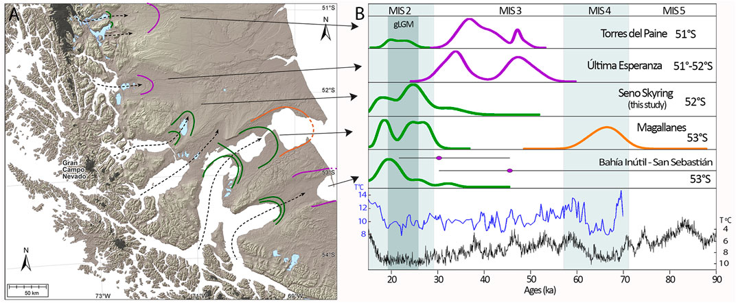
FIGURE 12. Southern Patagonia ice lobe extents and timing of occurrence of the moraine belts during the last glacial period from 15–90 ka. (A) Map of major moraine belts which are coloured to match the geochronology in panel (B). Orange corresponds to MIS 4, purple to MIS 3 and green to MIS 2. (B) Density functions (probability plots) of exposure ages of moraine boulders in Southern Patagonia moraine belts (this study; McCulloch et al., 2005b; Kaplan et al., 2008; Sagredo et al., 2011; García et al., 2018; Peltier et al., 2021). For the Bahía Inútil-San Sebastián ice lobe, the outer glacial margins were geochronological constrained through a cosmogenic nuclide depth profile approach performed on the outwash plain associated with their respective moraine (Darvill et al., 2015). These ages are indicated by a solid circle (purple) and their uncertainty by a horizontal line. The Sea Surface Temperature (SST) curve (blue) is from an off-shore core in northwestern Patagonia at 41°S (Kaiser et al., 2005) and the east Antarctic temperature record (black) from EPICA Dome C (Jouzel et al., 2007).

If we are to better understand the palaeoclimate of southernmost Patagonia two main questions need to be addressed: First, why do different lobes show different advance extension at similar times? Second, why does the timing of maximum extent differ between lobes?

There are a number of possible reasons for explaining the observed differences. First, there may be a sampling bias due to not all moraines being sampled. Second, there may be a preservation bias: particular moraine belts may have been eroded, overridden leading to an incomplete record of ice history. This is perhaps more likely to occur where there is a large MIS2 advance which may have eroded earlier landforms, which may be the case in Seno Skyring lobe. A third potential explanation is glaciological and topographic differences between ice lobes. For example, differences in basin geometry may control ice behaviour due to variations in the scale, shape and elevation distribution (hypsometry) of the ice drainage catchment (Furbish and Andrews, 1984; Kaplan et al., 2009; Anderson et al., 2012; Barr and Lovell, 2014), as may differences in substrate material (e.g., Benn and Clapperton, 2000b). A fourth set of explanations may lie in regional or local climatic differences. Understanding these influences could be best addressed through numerical modelling of the PIS. Nevertheless, here we provide some initial suggestions of potential explanations.

Patagonia is marked by strong W-E contrasts in precipitation (Garreaud, 2007). This contrast is caused by a rain shadow and continentality effects where the amount of precipitation falls rapidly as air masses rise over the Andes and move progressively east. The interplay of topography and precipitation may influence the geomorphic record of past glacial cycles. For example, those areas with higher elevation can grow more extensive glaciers because they have larger accumulation areas. This is the case for Torres del Paine, Última Esperanza, Magallanes and Bahía Inútil-San Sebastián lobes. These lobes also can start advancing earlier in a glacial cycle, having the potential to record older ice advances within the last glacial cycle. It is not the case where mountains are lower in their catchments, such as Seno Skyring and Seno Otway, since it will take more time for the area to be covered by ice and thus, spread away from the mountain zone (Sugden et al., 2002). Additionally, during the PIS build-up, higher areas will progressively develop an extensive ice sheet to the west (towards the precipitation source), producing the ice divide migration to the west, and provoking snow starvation effect to the east (Sugden et al., 2002). This can imply that during one glacial cycle, subsequent (younger) glacial advances reach more restricted positions, compared to previous advances (Mendelová et al., 2020). This will not be the case where altitudes of the mountains are lower, where the precipitation influence will affect the eastern area for a longer period, and younger glacial advances could have the potential to reach further positions beyond older advances. This could be one reason that in Seno Skyring, where the altitudes of the mountains are lower, the gLGM reaches close to maximum positions, and in the rest of Southern Patagonia, pre gLGM extents are significantly greater than gLGM limits. Moreover, the areas with lower mountains in their upper catchments may have a smaller orographic effect and so may experience greater precipitation over the glaciers.

5.6 Paleoclimate in Southernmost Patagonia

A cold temperature period prevailed during MIS 2 in Patagonia, according to Antarctic and Patagonian off-shore sea surface temperatures (SSTs) proxies (Blunier and Brook, 2001; Kaiser et al., 2005; Jouzel et al., 2007). The LB III and LB IV have ages of 26.3 ± 2.3 (n = 5) and 24.3 ± 0.9 ka (n = 3). LB III coincides with the onset of the gLGM and the coldest periods from East Antarctica. Moreover, the LB moraine ages are in agreement - within uncertainties -with the A limit moraine records from Magallanes ice lobe (Clapperton et al., 1995), dating to 25.7 ± 0.8 and 23.9 ± 0.8 (Peltier et al., 2021) and the C limit in Bahía Inútil-San Sebastián dating 23.2 ± 1.3 ka (McCulloch et al., 2005b; Figure 12). Humidity records in Patagonia during this period (e.g., Heusser et al., 1996; Moreno et al., 2015) suggest wetter conditions for the northern part of Patagonia, and drier for the south, implying a northern migration of the SWWs (Moreno et al., 1999; Hulton et al., 2002; Rojas et al., 2009). The wetter and colder conditions for north-central Patagonia are supported by the ice maxima in central-eastern Patagonia during the gLGM (Kaplan et al., 2004; Douglass et al., 2006; Hein et al., 2010; Leger et al., 2021). Despite the apparent reduction in the precipitation in southern Patagonia for the MIS 2 period, the PIS outlets advanced between about 100–250 km from present-day ice. Therefore, the precipitation in the area should have been sufficient alongside the sharp decrease in temperatures to develop full glacial conditions in the area. Peltier et al. (2021) suggest a mean annual temperature reduction in 4.5°C temperature, when a decrease in 25% of precipitation occurred for southernmost Patagonia during MIS 2.

By the end of the LGM and shortly before the onset of the last glacial termination, a less extensive glacial readvance, inboard from the LGM positions, and culminated at 18.7 ± 1.5 ka, represented in Seno Skyring by the RV moraine system. This broad pattern occurs for several other glacier outlets: in the Magallanes lobe, there are two short periods of glacial readvance/stillstand at 18.1 ± 0.8 and 19.1 ± 0.6 ka (Peltier et al., 2021) and a similar age for the “D limit” in Bahía Inútil-San Sebastián lobe with ages 19.7 ± 2.0 ka (McCulloch et al., 2005b; Kaplan et al., 2008). At Torres del Paine the TDP I moraine dates to 21.7 ± 2.0 ka (García et al., 2018). Considering the timings of these moraines within their uncertainties, there appears to be a close concordance in the timing of a readvance or stillstand at the end of the gLGM, showing a clear regional pattern.

After the RV moraine formation in Seno Skyring lobe, our geochronology shows that by c.16.4 cal kyr BP deglaciation was underway and by 14.8 ka, the glacier was already in the fjord area (Kilian et al., 2013). A synchronous retreat is observed in the Otway ice lobe, where Mercer (1970) reports a minimum deglaciation age of 14.6 cal kyr BP, for the ice abandonment close to the eastern shore of the Otway fjord (Figure 11F). Similarly, in the Magallanes and Bahía Inútil-San Sebastián lobes, deglaciation records suggest the glacier retreated to the northern part of Isla Dawson before c. 16.6 cal kr BP (Mcculloch and Bentley, 1998; McCulloch et al., 2005b). Other studies suggest that the glacier was already in the Darwin Cordillera by 16.8 ka, which corresponds to the accumulation area from Magallanes and Bahía Inútil-San Sebastián lobes (e.g., Hall et al., 2013; Hall et al., 2017; Hall et al., 2019). These deglaciation events follow a sharp climatic amelioration that occurred after ∼18 ka (Kaiser et al., 2005; Jouzel et al., 2007; Caniupán et al., 2011), which marks the onset of the last glacial termination in Patagonia also (Denton et al., 2010; Moreno et al., 2015). After the increase in temperature, at 18.1 ka the PIS experienced a rapid ice thinning (Boex et al., 2013) and an extraordinarily fast recession (Darvill et al., 2017; Davies et al., 2020; Moreno, 2020). By 14 ka the Seno Skyring ice lobe had retreated to the inner fjords close to Gran Campo Nevado, losing more than 80% of its length compared to its maximum of the last glacial cycle (Kilian et al., 2007).

6 Conclusion

Our geomorphology and geochronology reconstructions demonstrate that the Seno Skyring ice lobe reached full glacial conditions during the gLGM, marked by the LB III and IV advances by 26.3 ± 2.3 (n = 5) ka and 24.3 ± 0.9 ka (n = 3). During the ice retreat from the LB moraine system, a proglacial lake developed, which initially drained to the north. As the ice retreated, a new spillway opened towards the southeast by 22 ± 3 ka. A glacier readvance deposited the inboard RV moraines by 18.7 ± 1.5 ka (n = 6), before the onset of the deglaciation. By at least c.16.4 cal ky BP and from the whole RV system by c.14.9 cal ky BP.

We compare our new glacier record from Seno Skyring to published records from other lobes in southernmost Patagonia. There are differences in the morphostratigraphic pattern and timing of advances between lobes, with no single lobe recording all the advances seen regionally. We speculate that some of the differences in the ice extent throughout the last glacial period may be related to the snow starvation effect in response to a northward migration of the westerlies and/or a westward migration of the ice divide during the PIS build-up throughout the last glacial period. Nevertheless, right after the gLGM and before the Termination, broadly synchronic glacial advances with relatively reduced extents are recorded along southern Patagonia.

Data Availability Statement

The original contributions presented in the study are included in the article/Supplementary Material, further inquiries can be directed to the corresponding author.

Author Contributions

M-PL designed this manuscript project in discussion with J-LG, MB and SJ. M-PL analysed the data and drafted the manuscript with help from MB and J-LG. M-PL, J-LG, HF, MB and AH attended to fieldwork. CD contributed with sample information and their analysis. AH, HF, AR, DF, RS and SB contributed to the laboratory sample dating process. All authors discussed the results and contributed to the final manuscript.

Funding

M-PL holds the PhD studentship from ANID PFCHA/Doctorado Becas Chile/2018—72190469. The fieldwork campaigns and the majority of sample analysis were funded with the Chilean Grant FONDECYT #1161110 (J-LG). The ¹⁰Be depth profile sample process was funded with NERC CIAF grant 9199/1019 (MB; M-PL) and 9140/1013 (MB; CD). Gilchrist Educational Fund, Geography Department—Durham University; Norman Richardson Award—Ustinov College contributed to the fieldwork expenses of M-PL.

Conflict of Interest

The authors declare that the research was conducted in the absence of any commercial or financial relationships that could be construed as a potential conflict of interest.

Publisher’s Note

All claims expressed in this article are solely those of the authors and do not necessarily represent those of their affiliated organizations, or those of the publisher, the editors and the reviewers. Any product that may be evaluated in this article, or claim that may be made by its manufacturer, is not guaranteed or endorsed by the publisher.

Acknowledgments

We are grateful to Familia Vargas (Ea. Laguna Blanca), Familia Mclean (Ea. Las Charas) for the great support during fieldwork. We also thank Familia Concha (Ea. Ayelén), Ea. Cacique Mulato, Ea. La Leona, Ea. Entre Vientos, Ea. Divina Esperanza and Ea. El Ovejero for allowing us to access the field site. We thank Consuelo Antezana, Gabriel Gómez, Víctor García, Paulo Rodríguez, Tancrède Leger, Alex Mayne-Nicholls and Max Fischer for the assistance in the field. We thank Cristina Balaban and Pedro Guzmán for the useful discussions. Finally, we thank Sam Kelley and Nathan D. Stansell, two reviewers who made constructive comments on this paper.

Supplementary Material

The Supplementary Material for this article can be found online at: https://www.frontiersin.org/articles/10.3389/feart.2022.892316/full#supplementary-material

References

Anderson, R. S., Dühnforth, M., Colgan, W., and Anderson, L. (2012). Far-flung Moraines: Exploring the Feedback of Glacial Erosion on the Evolution of Glacier Length. Geomorphology 179, 269–285. doi:10.1016/j.geomorph.2012.08.018

CrossRef Full Text | Google Scholar

Balco, G., Stone, J. O., Lifton, N. A., and Dunai, T. J. (2008). A Complete and Easily Accessible Means of Calculating Surface Exposure Ages or Erosion Rates from 10Be and 26Al Measurements. Quat. Geochronol. 3 (3), 174–195. doi:10.1016/j.quageo.2007.12.001

CrossRef Full Text | Google Scholar

Barr, I. D., and Lovell, H. (2014). A Review of Topographic Controls on Moraine Distribution. Geomorphology 226, 44–64. doi:10.1016/j.geomorph.2014.07.030

CrossRef Full Text | Google Scholar

Benn, D. I., and Clapperton, C. M. (2000a). Glacial Sediment-Landform Associations and Paleoclimate during the Last Glaciation, Strait of Magellan, Chile. Quat. Res. 54 (1), 13–23. doi:10.1006/qres.2000.2140

CrossRef Full Text | Google Scholar

Benn, D. I., and Clapperton, C. M. (2000b). Pleistocene Glacitectonic Landforms and Sediments Around Central Magellan Strait, Southernmost Chile: Evidence for Fast Outlet Glaciers with Cold-Based Margins. Quat. Sci. Rev. 19 (6), 591–612. doi:10.1016/s0277-3791(99)00012-8

CrossRef Full Text | Google Scholar

Benn, D. (1996). Subglacial and Subaqueous Processes Near a Glacier Grounding Line: Sedimentological Evidence from a Former Ice‐dammed Lake, Achnasheen Scotland. Boreas 25 (1), 23–36.

Google Scholar

Bennett, M. R., and Glasser, N. F. (1991). The Glacial Landforms of Glen Geusachan, Cairngorms: a Reinterpretation. Scott. Geogr. Mag. 107 (2), 116–123. doi:10.1080/00369229118736819

CrossRef Full Text | Google Scholar

Bennett, M. R., Hambrey, M. J., Huddart, D., and Glasser, N. F. (1998). Glacial Thrusting & Moraine-Mound Formation in Svalbard & Britain: The Example of Coire a'Cheud-Chnoic (Valley of Hundred Hills), Torridon Scotland. J. Quat. Sci. 13 (6), 17–34.

Google Scholar

Blunier, T., and Brook, E. J. (2001). Timing of Millennial-Scale Climate Change in Antarctica and Greenland during the Last Glacial Period. science 291 (5501), 109–112. doi:10.1126/science.291.5501.109

PubMed Abstract | CrossRef Full Text | Google Scholar

Boex, J., Fogwill, C., Harrison, S., Glasser, N. F., Hein, A., Schnabel, C., et al. (2013). Rapid Thinning of the Late Pleistocene Patagonian Ice Sheet Followed Migration of the Southern Westerlies. Sci. Rep. 3 (1), 2118. doi:10.1038/srep02118

PubMed Abstract | CrossRef Full Text | Google Scholar

Caldenius, C. C. z. (1932). Las Glaciaciones Cuaternarias en la Patagonia y Tierra del Fuego. Geogr. Ann. 14 (1-2), 1–164. doi:10.2307/519583

CrossRef Full Text | Google Scholar

Caniupán, M., Lamy, F., Lange, C., Kaiser, J., Arz, H., Kilian, R., et al. (2011). Millennial‐scale Sea Surface Temperature and Patagonian Ice Sheet Changes off Southernmost Chile (53 S) over the Past∼ 60 Kyr. Paleoceanography 26 (3), 1-10. doi:10.1029/2010pa002049

CrossRef Full Text | Google Scholar

Chandler, B. M. P., Evans, D. J. A., Chandler, S. J. P., Ewertowski, M. W., Lovell, H., Roberts, D. H., et al. (2020). The Glacial Landsystem of Fjallsjökull, Iceland: Spatial and Temporal Evolution of Process-form Regimes at an Active Temperate Glacier. Geomorphology 361, 107192. doi:10.1016/j.geomorph.2020.107192

CrossRef Full Text | Google Scholar

Clapperton, C. M., Sugden, D. E., Kaufman, D. S., and McCulloch, R. D. (1995). The Last Glaciation in Central Magellan Strait, Southernmost Chile. Quat. Res. 44 (2), 133–148. doi:10.1006/qres.1995.1058

CrossRef Full Text | Google Scholar

Clapperton, C. (1993). Quaternary Geology and Geomorphology of South America. Amsterdam, Netherlands: Elsevier

Google Scholar

Clark, P. U., Dyke, A. S., Shakun, J. D., Carlson, A. E., Clark, J., Wohlfarth, B., et al. (2009). The Last Glacial Maximum. science 325 (5941), 710–714. doi:10.1126/science.1172873

PubMed Abstract | CrossRef Full Text | Google Scholar

Cogez, A., Herman, F., Pelt, É., Reuschlé, T., Morvan, G., Darvill, C. M., et al. (2018). U-th and &lt;sup&gt;10&lt;/sup&gt;Be Constraints on Sediment Recycling in Proglacial Settings, Lago Buenos Aires, Patagonia. Earth Surf. Dynam. 6 (1), 121–140. doi:10.5194/esurf-6-121-2018

CrossRef Full Text | Google Scholar

Darvill, C. M., Bentley, M. J., Stokes, C. R., Hein, A. S., and Rodés, Á. (2015). Extensive MIS 3 Glaciation in Southernmost Patagonia Revealed by Cosmogenic Nuclide Dating of Outwash Sediments. Earth Planet. Sci. Lett. 429, 157–169. doi:10.1016/j.epsl.2015.07.030

CrossRef Full Text | Google Scholar

Darvill, C. M., Bentley, M. J., Stokes, C. R., and Shulmeister, J. (2016). The Timing and Cause of Glacial Advances in the Southern Mid-latitudes during the Last Glacial Cycle Based on a Synthesis of Exposure Ages from Patagonia and New Zealand. Quat. Sci. Rev. 149, 200–214. doi:10.1016/j.quascirev.2016.07.024

CrossRef Full Text | Google Scholar

Darvill, C. M., Stokes, C. R., Bentley, M. J., Evans, D. J. A., and Lovell, H. (2017). Dynamics of Former Ice Lobes of the Southernmost Patagonian Ice Sheet Based on a Glacial Landsystems Approach. J. Quat. Sci. 32 (6), 857–876. doi:10.1002/jqs.2890

CrossRef Full Text | Google Scholar

Darvill, C. M., Stokes, C. R., Bentley, M. J., and Lovell, H. (2014). A Glacial Geomorphological Map of the Southernmost Ice Lobes of Patagonia: the Bahía Inútil - San Sebastián, Magellan, Otway, Skyring and Río Gallegos Lobes. J. Maps 10 (3), 500–520. doi:10.1080/17445647.2014.890134

CrossRef Full Text | Google Scholar

Davies, B. J., Darvill, C. M., Lovell, H., Bendle, J. M., Dowdeswell, J. A., Fabel, D., et al. (2020). The Evolution of the Patagonian Ice Sheet from 35 Ka to the Present Day (PATICE). Earth-Science Rev. 204, 103152. doi:10.1016/j.earscirev.2020.103152

CrossRef Full Text | Google Scholar

Davies, B. J., Thorndycraft, V. R., Fabel, D., and Martin, J. R. V. (2018). Asynchronous Glacier Dynamics during the Antarctic Cold Reversal in Central Patagonia. Quat. Sci. Rev. 200, 287–312. doi:10.1016/j.quascirev.2018.09.025

CrossRef Full Text | Google Scholar

Denton, G. H., Anderson, R. F., Toggweiler, J. R., Edwards, R. L., Schaefer, J. M., and Putnam, A. E. (2010). The Last Glacial Termination. science 328 (5986), 1652–1656. doi:10.1126/science.1184119

PubMed Abstract | CrossRef Full Text | Google Scholar

Dewald, A., Heinze, S., Jolie, J., Zilges, A., Dunai, T., Rethemeyer, J., et al. (2013). CologneAMS, a Dedicated Center for Accelerator Mass Spectrometry in Germany, Nuclear Instruments. Methods in Physics Research Section B: Beam Interactions with Materials and Atoms, 294, 18–23. doi:10.1016/j.nimb.2012.04.030

CrossRef Full Text | Google Scholar

Douglass, D. C., Singer, B. S., Ackert, R. P., Stone, J., Kaplan, M. R., and Caffee, M. (2007). “Constraining Boulder Erosion Rates and Ages of Mid-pleistocene Moraines. In Lago Buenos Aires, Argentina,” in GSA Abstracts and Programs Northeastern Section, 42nd Annual Meeting. Durham, New Hampshire

Google Scholar

Douglass, D., Singer, B., Kaplan, M., Mickelson, D., and Caffee, M. (2006). Cosmogenic Nuclide Surface Exposure Dating of Boulders on Last-Glacial and Late-Glacial Moraines, Lago Buenos Aires, Argentina: Interpretive Strategies and Paleoclimate Implications. Quat. Geochronol. 1 (1), 43–58. doi:10.1016/j.quageo.2006.06.001

CrossRef Full Text | Google Scholar

Evans, D. (2003a). Glacial Landsystems. London: Hodder Arnold.

Google Scholar

Evans, D. (2003b). “Ice-marginal Terrestrial Landsystems: Active Temperate Glacier Margins,” in Glacial Landsystems. London, UK: Arnold, 12–43.

Google Scholar

Evans, D. J. A., and England, J. (1991). High Arctic Thrust Block Moraines. Can. Geogr. 35 (1), 93–97. doi:10.1111/j.1541-0064.1991.tb01628.x

CrossRef Full Text | Google Scholar

Evans, D. J., and Benn, D. I. (2021). A Practical Guide to the Study of Glacial Sediments. London: QRA.

Google Scholar

Evans, D. J., and Twigg, D. R. (2002). The Active Temperate Glacial Landsystem: a Model Based on Breiðamerkurjökull and Fjallsjökull, Iceland. Quat. Sci. Rev. 21 (20-22), 2143–2177. doi:10.1016/s0277-3791(02)00019-7

CrossRef Full Text | Google Scholar

Furbish, D. J., and Andrews, J. T. (1984). The Use of Hypsometry to Indicate Long-Term Stability and Response of Valley Glaciers to Changes in Mass Transfer. J. Glaciol. 30 (105), 199–211. doi:10.3189/s0022143000005931

CrossRef Full Text | Google Scholar

García, J.-L., Hall, B. L., Kaplan, M. R., Gómez, G. A., De Pol-Holz, R., García, V. J., et al. (2020). 14C and 10Be dated Late Holocene fluctuations of Patagonian glaciers in Torres del Paine (Chile, 51°S) and connections to Antarctic climate change. Quat. Sci. Rev. 246, 106541. doi:10.1016/j.quascirev.2020.106541

CrossRef Full Text | Google Scholar

García, J.-L., Hein, A. S., Binnie, S. A., Gómez, G. A., González, M. A., and Dunai, T. J. (2018). The MIS 3 maximum of the Torres del Paine and Última Esperanza ice lobes in Patagonia and the pacing of southern mountain glaciation. Quat. Sci. Rev. 185, 9–26. doi:10.1016/j.quascirev.2018.01.013

CrossRef Full Text | Google Scholar

García, J.-L., Lüthgens, C., Vega, R. M., Rodés, Á., Hein, A., and Binnie, S. (2021). A composite 10Be, IR-50 and 14C chronology of the pre-LGM full ice extent of the western Patagonian Ice Sheet in the Isla de Chiloé, south Chile (42°S). E&G-Quaternary Sci. J. 70 (1). doi:10.5194/egqsj-70-105-2021

CrossRef Full Text | Google Scholar

García, J.-L., Strelin, J. A., Vega, R. M., Hall, B. L., and Stern, C. R. (2015). Deglacial ice-marginal glaciolacustrine environments and structural moraine building in Torres del Paine, Chilean southern Patagonia. Andean Geol. 42 (2), 190–212. doi:10.5027/andgeov42n2-a03

CrossRef Full Text | Google Scholar

Garreaud, R. D. (2009). The Andes Climate and Weather. Adv. Geosci. 22, 3–11. doi:10.5194/adgeo-22-3-2009

CrossRef Full Text | Google Scholar

Garreaud, R., Lopez, P., Minvielle, M., and Rojas, M. (2013). Large-scale Control on the Patagonian Climate. J. Clim. 26 (1), 215–230. doi:10.1175/jcli-d-12-00001.1

CrossRef Full Text | Google Scholar

Garreaud, R. (2007). Precipitation and Circulation Covariability in the Extratropics. J. Clim. 20 (18), 4789–4797. doi:10.1175/jcli4257.1

CrossRef Full Text | Google Scholar

Glasser, N. F., and Hambrey, M. J. (2002). Sedimentary Facies and Landform Genesis at a Temperate Outlet Glacier: Soler Glacier, North Patagonian Icefield. Sedimentology 49 (1), 43–64. doi:10.1046/j.1365-3091.2002.00431.x

CrossRef Full Text | Google Scholar

Glasser, N. F., Jansson, K. N., Harrison, S., and Kleman, J. (2008). The Glacial Geomorphology and Pleistocene History of South America between 38 S and 56 S. Quat. Sci. Rev. 27 (3-4), 365–390. doi:10.1016/j.quascirev.2007.11.011

CrossRef Full Text | Google Scholar

Glasser, N., and Jansson, K. (2008). The Glacial Map of Southern South America. J. Maps 4 (1), 175–196. doi:10.4113/jom.2008.1020

CrossRef Full Text | Google Scholar

Glasser, N. S., and Hambrey, M. J. (2003). “Ice-marginal Terrestrial Landsystems: Svalbard Polythermal Glaciers,” in Glacial Landsystems (London: Arnold), 228, 258.

Google Scholar

Gosse, J. C., and Phillips, F. M. (2001). Terrestrial In Situ Cosmogenic Nuclides: Theory and Application. Quat. Sci. Rev. 20 (14), 1475–1560. doi:10.1016/s0277-3791(00)00171-2

CrossRef Full Text | Google Scholar

Hall, B. L., Denton, G., Lowell, T., Bromley, G. R. M., and Putnam, A. E. (2017). Retreat of the Cordillera Darwin Icefield during Termination I. Cig 43, 751–766. doi:10.18172/cig.3158

CrossRef Full Text | Google Scholar

Hall, B. L., Lowell, T. V., Bromley, G. R. M., Denton, G. H., and Putnam, A. E. (2019). Holocene Glacier Fluctuations on the Northern Flank of Cordillera Darwin, Southernmost South America. Quat. Sci. Rev. 222, 105904. doi:10.1016/j.quascirev.2019.105904

CrossRef Full Text | Google Scholar

Hall, B. L., Porter, C. T., Denton, G. H., Lowell, T. V., and Bromley, G. R. M. (2013). Extensive Recession of Cordillera Darwin Glaciers in Southernmost South America during Heinrich Stadial 1. Quat. Sci. Rev. 62, 49–55. doi:10.1016/j.quascirev.2012.11.026

CrossRef Full Text | Google Scholar

Hambrey, M. J., Huddart, D., Bennett, M. R., and Glasser, N. F. (1997). Genesis of 'hummocky Moraines' by Thrusting in Glacier Ice: Evidence from Svalbard and Britain. J. Geol. Soc. 154 (4), 623–632. doi:10.1144/gsjgs.154.4.0623

CrossRef Full Text | Google Scholar

Hancock, G. S., Anderson, R. S., Chadwick, O. A., and Finkel, R. C. (1999). Dating Fluvial Terraces with 10Be and 26Al Profiles: Application to the Wind River, Wyoming. Geomorphology 27 (1-2), 41–60. doi:10.1016/s0169-555x(98)00089-0

CrossRef Full Text | Google Scholar

Hein, A. S., Dunai, T. J., Hulton, N. R. J., and Xu, S. (2011). Exposure Dating Outwash Gravels to Determine the Age of the Greatest Patagonian Glaciations. Geology 39 (2), 103–106. doi:10.1130/g31215.1

CrossRef Full Text | Google Scholar

Hein, A. S., Hulton, N. R., Dunai, T. J., Schnabel, C., Kaplan, M. R., Naylor, M., et al. (2009). Middle Pleistocene Glaciation in Patagonia Dated by Cosmogenic-Nuclide Measurements on Outwash Gravels. Earth Planet. Sci. Lett. 286 (1-2), 184–197. doi:10.1016/j.epsl.2009.06.026

CrossRef Full Text | Google Scholar

Hein, A. S., Hulton, N. R., Dunai, T. J., Sugden, D. E., Kaplan, M. R., and Xu, S. (2010). The Chronology of the Last Glacial Maximum and Deglacial Events in Central Argentine Patagonia. Quat. Sci. Rev. 29 (9-10), 1212–1227. doi:10.1016/j.quascirev.2010.01.020

CrossRef Full Text | Google Scholar

Heusser, C. J., Lowell, T. V., Heusser, L. E., Hauser, A., Andersen, B. G., and Denton, G. H. (1996). Full-glacial - Late-Glacial Palaeoclimate of the Southern Andes: Evidence from Pollen, Beetle and Glacial Records. J. Quat. Sci. 11 (3), 173–184. doi:10.1002/(sici)1099-1417(199605/06)11:3<173:aid-jqs237>3.0.co;2-5

CrossRef Full Text | Google Scholar

Heyman, J., Applegate, P. J., Blomdin, R., Gribenski, N., Harbor, J. M., and Stroeven, A. P. (2016). Boulder Height–Exposure Age Relationships from a Global Glacial 10Be Compilation. Quaternary Geochronol. 34, 1–11.

CrossRef Full Text | Google Scholar

Hidy, A. J., Gosse, J. C., Pederson, J. L., Mattern, J. P., and Finkel, R. C. (2010). A Geologically Constrained Monte Carlo Approach to Modeling Exposure Ages from Profiles of Cosmogenic Nuclides: An Example from Lees Ferry, Arizona. Geochem. Geophys. Geosystems 11 (9). doi:10.1029/2010gc003084

CrossRef Full Text | Google Scholar

Hogg, A. G., Heaton, T. J., Hua, Q., Palmer, J. G., Turney, C. S., Southon, J., et al. (2020). SHCal20 Southern Hemisphere Calibration, 0-55,000 Years Cal BP. Radiocarbon 62 (4), 759–778. doi:10.1017/rdc.2020.59

CrossRef Full Text | Google Scholar

Hulton, N. R., Purves, R., McCulloch, R., Sugden, D. E., and Bentley, M. J. (2002). The Last Glacial Maximum and Deglaciation in Southern South America. Quat. Sci. Rev. 21 (1-3), 233–241. doi:10.1016/s0277-3791(01)00103-2

CrossRef Full Text | Google Scholar

Johnson, M., and Clayton, L. (2003). “Supraglacial Landsystems in Lowland Terrain,” in Glacial Landsystems (London: Arnold), 228–258.

Google Scholar

Jones, R. S., Small, D., Cahill, N., Bentley, M. J., and Whitehouse, P. L. (2019). iceTEA: Tools for Plotting and Analysing Cosmogenic-Nuclide Surface-Exposure Data from Former Ice Margins. Quat. Geochronol. 51, 72–86. doi:10.1016/j.quageo.2019.01.001

CrossRef Full Text | Google Scholar

Jouzel, J., Masson-Delmotte, V., Cattani, O., Dreyfus, G., Falourd, S., Hoffmann, G., et al. (2007). Orbital and Millennial Antarctic Climate Variability over the Past 800,000 Years. science 317 (5839), 793–796. doi:10.1126/science.1141038

PubMed Abstract | CrossRef Full Text | Google Scholar

Kaiser, J., Lamy, F., and Hebbeln, D. (2005). A 70‐kyr Sea Surface Temperature Record off Southern Chile (Ocean Drilling Program Site 1233). Paleoceanography 20 (4), 1-15. doi:10.1029/2005pa001146

CrossRef Full Text | Google Scholar

Kaplan, M., Fogwill, C., Sugden, D., Hulton, N., Kubik, P., and Freeman, S. (2008). Southern Patagonian Glacial Chronology for the Last Glacial Period and Implications for Southern Ocean Climate. Quat. Sci. Rev. 27 (3-4), 284–294. doi:10.1016/j.quascirev.2007.09.013

CrossRef Full Text | Google Scholar

Kaplan, M. R., Ackert, R. P., Singer, B. S., Douglass, D. C., and Kurz, M. D. (2004). Cosmogenic Nuclide Chronology of Millennial-Scale Glacial Advances during O-Isotope Stage 2 in Patagonia. Geol. Soc. Am. Bull. 116 (3-4), 308–321. doi:10.1130/b25178.1

CrossRef Full Text | Google Scholar

Kaplan, M. R., Douglass, D. C., Singer, B. S., Ackert, R. P., and Caffee, M. W. (2005). Cosmogenic Nuclide Chronology of Pre-last Glacial Maximum Moraines at Lago Buenos Aires, 46 S, Argentina. Quat. Res. 63 (3), 301–315. doi:10.1016/j.yqres.2004.12.003

CrossRef Full Text | Google Scholar

Kaplan, M. R., Hein, A. S., Hubbard, A., and Lax, S. M. (2009). Can Glacial Erosion Limit the Extent of Glaciation? Geomorphology 103 (2), 172–179. doi:10.1016/j.geomorph.2008.04.020

CrossRef Full Text | Google Scholar

Kaplan, M. R., Strelin, J. A., Schaefer, J. M., Denton, G. H., Finkel, R. C., Schwartz, R., et al. (2011). In-situ Cosmogenic 10Be Production Rate at Lago Argentino, Patagonia: Implications for Late-Glacial Climate Chronology. Earth Planet. Sci. Lett. 309 (1-2), 21–32. doi:10.1016/j.epsl.2011.06.018

CrossRef Full Text | Google Scholar

Kilian, R., Baeza, O., Breuer, S., Ríos, F., Arz, H., Lamy, F., et al. (2013). Late Glacial and Holocene Paleogeographical and Paleoecological Evolution of the Seno Skyring and Otway Fjord Systems in the Magellan Region. An. Inst. Patagon. (Chile) 41 (2), 5–26. doi:10.4067/s0718-686x2013000200001

CrossRef Full Text | Google Scholar

Kilian, R., Schneider, C., Koch, J., Fesq-Martin, M., Biester, H., Casassa, G., et al. (2007). Palaeoecological Constraints on Late Glacial and Holocene Ice Retreat in the Southern Andes (53 S). Glob. Planet. Change 59 (1-4), 49–66. doi:10.1016/j.gloplacha.2006.11.034

CrossRef Full Text | Google Scholar

Lal, D. (1991). Cosmic Ray Labeling of Erosion Surfaces: In Situ Nuclide Production Rates and Erosion Models. Earth Planet. Sci. Lett. 104 (2-4), 424–439. doi:10.1016/0012-821x(91)90220-c

CrossRef Full Text | Google Scholar

Lambeck, K., Rouby, H., Purcell, A., Sun, Y., and Sambridge, M. (2014). Sea Level and Global Ice Volumes from the Last Glacial Maximum to the Holocene. Proc. Natl. Acad. Sci. U.S.A. 111 (43), 15296–15303. doi:10.1073/pnas.1411762111

PubMed Abstract | CrossRef Full Text | Google Scholar

Lamy, F., Kilian, R., Arz, H. W., Francois, J.-P., Kaiser, J., Prange, M., et al. (2010). Holocene Changes in the Position and Intensity of the Southern Westerly Wind Belt. Nat. Geosci. 3 (10), 695–699. doi:10.1038/ngeo959

CrossRef Full Text | Google Scholar

Leger, T. P. M., Hein, A. S., Bingham, R. G., Rodés, Á., Fabel, D., and Smedley, R. K. (2021). Geomorphology and 10Be Chronology of the Last Glacial Maximum and Deglaciation in Northeastern Patagonia, 43°S-71°W. Quat. Sci. Rev. 272, 107194. doi:10.1016/j.quascirev.2021.107194

CrossRef Full Text | Google Scholar

Lifton, N., Sato, T., and Dunai, T. J. (2014). Scaling In Situ Cosmogenic Nuclide Production Rates Using Analytical Approximations to Atmospheric Cosmic-Ray Fluxes. Earth Planet. Sci. Lett. 386, 149–160. doi:10.1016/j.epsl.2013.10.052

CrossRef Full Text | Google Scholar

Lovell, H., Stokes, C. R., and Bentley, M. J. (2011). A Glacial Geomorphological Map of the Seno Skyring-Seno Otway-Strait of Magellan Region, Southernmost Patagonia. J. Maps 7 (1), 318–339. doi:10.4113/jom.2011.1156

CrossRef Full Text | Google Scholar

Lovell, H., Stokes, C. R., Bentley, M. J., and Benn, D. I. (2012). Evidence for Rapid Ice Flow and Proglacial Lake Evolution Around the Central Strait of Magellan Region, Southernmost Patagonia. J. Quat. Sci. 27 (6), 625–638. doi:10.1002/jqs.2555

CrossRef Full Text | Google Scholar

Manger, G. (1963). “Porosity and Bulk Density of Sedimentary Rocks,” in Geological Survey Bulletin (Washington D.C.: US Atomic Energy Commission), 1144.

Google Scholar

Mcculloch, R. D., and Bentley, M. J. (1998). Late Glacial Ice Advances in the Strait of Magellan, Southern Chile. Quat. Sci. Rev. 17 (8), 775–787. doi:10.1016/s0277-3791(97)00074-7

CrossRef Full Text | Google Scholar

McCulloch, R. D., Bentley, M. J., Tipping, R. M., and Clapperton, C. M. (2005a). Evidence for Late‐glacial Ice Dammed Lakes in the Central Strait of Magellan and Bahía Inútil, Southernmost South america. Geogr. Ann. Ser. A, Phys. Geogr. 87 (2), 335–362. doi:10.1111/j.0435-3676.2005.00262.x

CrossRef Full Text | Google Scholar

McCulloch, R. D., Blaikie, J., Jacob, B., Mansilla, C. A., Morello, F., De Pol-Holz, R., et al. (2020). Late Glacial and Holocene Climate Variability, Southernmost Patagonia. Quat. Sci. Rev. 229, 106131. doi:10.1016/j.quascirev.2019.106131

CrossRef Full Text | Google Scholar

McCulloch, R. D., Fogwill, C. J., Sugden, D. E., Bentley, M. J., and Kubik, P. W. (2005b). Chronology of the Last Glaciation in Central Strait of Magellan and Bahía Inútil, Southernmost South america. Geogr. Ann. Ser. A, Phys. Geogr. 87 (2), 289–312. doi:10.1111/j.0435-3676.2005.00260.x

CrossRef Full Text | Google Scholar

Meglioli, A. (1992). Glacial geology and chronology of southernmost Patagonia and Tierra del Fuego, Argentina and Chile (Lehigh University). PhD thesis. Bethlehem, Pennsylvania.

Mendelová, M., Hein, A. S., Rodés, Á., and Xu, S. (2020). Extensive Mountain Glaciation in Central Patagonia during Marine Isotope Stage 5. Quat. Sci. Rev. 227, 105996. doi:10.1016/j.quascirev.2019.105996

CrossRef Full Text | Google Scholar

Mercer, J. H. (1970). Variations of Some Patagonian Glaciers since the Late-Glacial; II. Am. J. Sci. 269 (1), 1–25. doi:10.2475/ajs.269.1.1

CrossRef Full Text | Google Scholar

Moreno, P. I., Denton, G. H., Moreno, H., Lowell, T. V., Putnam, A. E., and Kaplan, M. R. (2015). Radiocarbon Chronology of the Last Glacial Maximum and its Termination in Northwestern Patagonia. Quat. Sci. Rev. 122, 233–249. doi:10.1016/j.quascirev.2015.05.027

CrossRef Full Text | Google Scholar

Moreno, P. I., Lowell, T. V., Jacobson Jr, G. L., and Denton, G. H. (1999). Abrupt Vegetation and Climate Changes during the Last Glacial Maximumand Last Termination in the Chilean Lake District: A Case Study from Canal De La Puntilla (41oS). Geogr. Ann. A 81 (2), 285–311. doi:10.1111/j.0435-3676.1999.00059.x

CrossRef Full Text | Google Scholar

Moreno, P. I. (2020). Timing and Structure of Vegetation, Fire, and Climate Changes on the Pacific Slope of Northwestern Patagonia since the Last Glacial Termination. Quat. Sci. Rev. 238, 106328. doi:10.1016/j.quascirev.2020.106328

CrossRef Full Text | Google Scholar

Nishiizumi, K., Imamura, M., Caffee, M. W., Southon, J. R., Finkel, R. C., and McAninch, J. (2007). Absolute Calibration of 10Be AMS Standards. Nucl. Instrum. Methods Phys. Res. Sect. B Beam Interact. Mater. Atoms 258 (2), 403–413. doi:10.1016/j.nimb.2007.01.297

CrossRef Full Text | Google Scholar

Peltier, C., Kaplan, M. R., Birkel, S. D., Soteres, R. L., Sagredo, E. A., Aravena, J. C., et al. (2021). The Large MIS 4 and Long MIS 2 Glacier Maxima on the Southern Tip of South America. Quat. Sci. Rev. 262, 106858. doi:10.1016/j.quascirev.2021.106858

CrossRef Full Text | Google Scholar

Quik, C., Velde, Y., Harkema, T., Plicht, H., Quik, J., Beek, R., et al. (2021). Using Legacy Data to Reconstruct the Past? Rescue, Rigour and Reuse in Peatland Geochronology. Earth Surf. Process. Landf. 46 (13), 2607–2631. doi:10.1002/esp.5196

CrossRef Full Text | Google Scholar

Rabassa, J. (2008). Late cenozoic glaciations in Patagonia and Tierra del Fuego. Dev. Quat. Sci. 11, 151–204. doi:10.1016/s1571-0866(07)10008-7

CrossRef Full Text | Google Scholar

Rodés, Á., Pallàs, R., Braucher, R., Moreno, X., Masana, E., and Bourlés, D. L. (2011). Effect of Density Uncertainties in Cosmogenic 10Be Depth-Profiles: Dating a Cemented Pleistocene Alluvial Fan (Carboneras Fault, SE Iberia). Quat. Geochronol. 6 (2), 186–194. doi:10.1016/j.quageo.2010.10.004

CrossRef Full Text | Google Scholar

Rodés, Á., Pallàs, R., Ortuño, M., García-Melendez, E., and Masana, E. (2014). Combining Surface Exposure Dating and Burial Dating from Paired Cosmogenic Depth Profiles. Example of El Límite Alluvial Fan in Huércal-Overa Basin (SE Iberia). Quat. Geochronol. 19, 127–134. doi:10.1016/j.quageo.2013.10.002

CrossRef Full Text | Google Scholar

Rojas, M., Moreno, P., Kageyama, M., Crucifix, M., Hewitt, C., Abe-Ouchi, A., et al. (2009). The Southern Westerlies during the Last Glacial Maximum in PMIP2 Simulations. Clim. Dyn. 32 (4), 525–548. doi:10.1007/s00382-008-0421-7

CrossRef Full Text | Google Scholar

Ruppel, M., Väliranta, M., Virtanen, T., and Korhola, A. (2013). Postglacial Spatiotemporal Peatland Initiation and Lateral Expansion Dynamics in North America and Northern Europe. Holocene 23 (11), 1596–1606. doi:10.1177/0959683613499053

CrossRef Full Text | Google Scholar

Sagredo, E. A., Moreno, P. I., Villa-Martínez, R., Kaplan, M. R., Kubik, P. W., and Stern, C. R. (2011). Fluctuations of the Última Esperanza Ice Lobe (52°S), Chilean Patagonia, during the Last Glacial Maximum and Termination 1. Geomorphology 125 (1), 92–108. doi:10.1016/j.geomorph.2010.09.007

CrossRef Full Text | Google Scholar

Sigfúsdóttir, T., Benediktsson, Í. Ö., and Phillips, E. (2018). Active Retreat of a Late Weichselian Marine-Terminating Glacier: an Example from Melasveit, Western Iceland. Boreas 47 (3), 813–836. doi:10.1111/bor.12306

CrossRef Full Text | Google Scholar

Singer, B. S., Ackert, R. P., and Guillou, H. (2004). 40Ar/39Ar and K-Ar Chronology of Pleistocene Glaciations in Patagonia. Geol. Soc. Am. Bull. 116 (3-4), 434–450. doi:10.1130/b25177.1

CrossRef Full Text | Google Scholar

Smedley, R. K., Glasser, N. F., and Duller, G. A. T. (2016). Luminescence Dating of Glacial Advances at Lago Buenos Aires (∼46 °S), Patagonia. Quat. Sci. Rev. 134, 59–73. doi:10.1016/j.quascirev.2015.12.010

CrossRef Full Text | Google Scholar

Spencer, C. J., Yakymchuk, C., and Ghaznavi, M. (2017). Visualising Data Distributions with Kernel Density Estimation and Reduced Chi-Squared Statistic. Geosci. Front. 8 (6), 1247–1252.

CrossRef Full Text | Google Scholar

Stern, C. R., Moreno, P. I., Villa-Martínez, R., Sagredo, E. A., Prieto, A., and Labarca, R. (2011). Evolution of Ice-Dammed Proglacial Lakes in Última Esperanza, Chile: Implications from the Late-Glacial R1 Eruption of Reclús Volcano, Andean Austral Volcanic Zone. Andean Geol. 38 (1), 82–97. doi:10.5027/andgeov38n1-a06

CrossRef Full Text | Google Scholar

Stone, J. O. (2000). Air Pressure and Cosmogenic Isotope Production. J. Geophys. Res. 105 (B10), 23753–23759. doi:10.1029/2000jb900181

CrossRef Full Text | Google Scholar

Stuiver, M., Reimer, P., and Reimer, R. (2021). CALIB 8.2. [WWW program] at http://calib.org. Accessed 2022-04-1.

Google Scholar

Sugden, D. E., Hulton, N. R. J., and Purves, R. S. (2002). Modelling the Inception of the Patagonian Icesheet. Quat. Int. 95-96, 55–64. doi:10.1016/s1040-6182(02)00027-7

CrossRef Full Text | Google Scholar

Sugden, D. E., McCulloch, R. D., Bory, A. J.-M., and Hein, A. S. (2009). Influence of Patagonian Glaciers on Antarctic Dust Deposition during the Last Glacial Period. Nat. Geosci. 2 (4), 281–285. doi:10.1038/ngeo474

CrossRef Full Text | Google Scholar

Thorndycraft, V. R., Bendle, J. M., Benito, G., Davies, B. J., Sancho, C., Palmer, A. P., et al. (2019). Glacial Lake Evolution and Atlantic-Pacific Drainage Reversals during Deglaciation of the Patagonian Ice Sheet. Quat. Sci. Rev. 203, 102–127. doi:10.1016/j.quascirev.2018.10.036

CrossRef Full Text | Google Scholar

Troch, M., Bertrand, S., Lange, C. B., Cárdenas, P., Arz, H., Pantoja-Gutiérrez, S., et al. (2022). Glacial Isostatic Adjustment Near the Center of the Former Patagonian Ice Sheet (48°S) during the Last 16.5 Kyr. Quat. Sci. Rev. 277, 107346. doi:10.1016/j.quascirev.2021.107346

CrossRef Full Text | Google Scholar

Tuhkanen, S., Kuokka, I., Hyvönen, J., Stenroos, S., and Niemelä, J. (1989-1990). Tierra del Fuego as a target for biogeographical research in the past and present. Anales del Instituto de la Patagonia Serie Ciencias Naturales 19 (2), 1–107.

Google Scholar

Wendt, I., and Carl, C. (1991). The Statistical Distribution of the Mean Squared Weighted Deviation. Chem. Geol. Isot. Geosci. Sect. 86 (4), 275–285. doi:10.1016/0168-9622(91)90010-t

CrossRef Full Text | Google Scholar

Zolitschka, B., Francus, P., Ojala, A. E. K., and Schimmelmann, A. (2015). Varves in Lake Sediments - a Review. Quat. Sci. Rev. 117, 1–41. doi:10.1016/j.quascirev.2015.03.019

CrossRef Full Text | Google Scholar