Abstract
Accurate prediction of water inrush volumes is essential for safeguarding tunnel construction operations. This study proposes a method for predicting tunnel water inrush volumes, leveraging the eXtreme Gradient Boosting (XGBoost) model optimized with Bayesian techniques. To maximize the utility of available data, 654 datasets with missing values were imputed and augmented, forming a robust dataset for the training and validation of the Bayesian optimized XGBoost (BO-XGBoost) model. Furthermore, the SHapley Additive explanations (SHAP) method was employed to elucidate the contribution of each input feature to the predictive outcomes. The results indicate that: (1) The constructed BO-XGBoost model exhibited exceptionally high predictive accuracy on the test set, with a root mean square error (RMSE) of 7.5603, mean absolute error (MAE) of 3.2940, mean absolute percentage error (MAPE) of 4.51%, and coefficient of determination (R2) of 0.9755; (2) Compared to the predictive performance of support vector mechine (SVR), decision tree (DT), and random forest (RF) models, the BO-XGBoost model demonstrates the highest R2 values and the smallest prediction error; (3) The input feature importance yielded by SHAP is groundwater level (h) > water-producing characteristics (W) > tunnel burial depth (H) > rock mass quality index (RQD). The proposed BO-XGBoost model exhibited exceptionally high predictive accuracy on the tunnel water inrush volume prediction dataset, thereby aiding managers in making informed decisions to mitigate water inrush risks and ensuring the safe and efficient advancement of tunnel projects.
1 Introduction
Tunnels constitute a prevalent form of underground infrastructure, the construction of which entails a multitude of risks and challenges (Kim J. et al., 2022; Liu et al., 2022). Tunnel water inflow (WI) represents a common geological calamity within tunnels, posing a significant threat to the safety of construction personnel and machinery within the tunnel and substantially impeding the safe and efficient construction of tunnels (Li and Wu, 2019; Wang et al., 2020). The occurrence of WI attributes to a variety of complex factors (Golian et al., 2018; Farhadian and Nikvar-Hassani, 2019). The primary causes include: (1) the intricate geological conditions, such as fractured rock strata, well-developed fractures, and extensive karst formations, which facilitate the easy ingress of groundwater during tunnel excavation (Jin et al., 2016); (2) the adverse hydrogeological conditions, such as high groundwater levels and hydraulic connectivity between surface water and groundwater, which increase the likelihood of WI; and (3) human-related factors during construction, such as improper construction methods and inadequate support designs, which may also trigger water gushing hazards. The WI disaster in tunnels poses severe and multifaceted risks (Li et al., 2017). First and foremost, it directly threatens the safety of construction personnel, potentially causing casualties and equipment damage. Secondly, the inflow of water increases construction difficulty and reduces construction efficiency, leading to delays in project timelines and increased costs. Additionally, prolonged water immersion weakens the stability of tunnel structures, leaving safety hazards and negatively impacting the tunnel’s service life. Globally, hundreds of tunnel water inflow incidents have transpired, inflicting substantial casualties and economic losses across various countries and regions (Holmøy and Nilsen, 2014). For instance, on 5 August 2007, a large-scale water inflow incident occurred in the Youshanguan Tunnel of the Yichang-Wanzhou Railway in China, resulting in considerable losses and difficulties in tunnel construction (Jin et al., 2016). To mitigate or avert the damage precipitated by water inflow disasters during tunnel construction, a pivotal task is to assess the tunnel water inflow volume prior to tunnel excavation, thereby enabling the formulation of appropriate contingency plans to prevent or control water inflow (Farhadian and Nikvar-Hassani, 2019).
In recent years, scholars have conducted extensive research on predicting tunnel water inflow volumes, primarily employing theoretical analysis, empirical methods, and numerical simulation techniques (Hwang and Lu, 2007; Holmøy and Nilsen, 2014; Farhadian and Katibeh, 2017; Golian et al., 2018). While theoretical analysis methods are convenient and quick, their predictive accuracy is limited due to reliance on simplistic circular or rectangular interfaces, particularly when dealing with complex hydrogeological parameters such as rock fractures. With the rapid advancement of computer technology, numerous numerical computation methods have been developed to study tunnel water inflow volumes (Berkowitz, 2002; Yao et al., 2012). However, the difficulty in obtaining accurate hydrological and geological data often results in numerical simulations that fail to precisely replicate the actual water inflow environment and calculate the water inflow volume accurately. Additionally, the numerous assumptions and simplifications made during the construction of numerical models can reduce the accuracy of the computational results. Tunnel water inflow volume is influenced by a multitude of factors, including hydrological and geological conditions, making it a significant challenge to accurately predict using traditional research methods.
As an emerging computational approach, machine learning (ML) methods hold great potential in handling the complex nonlinear relationships in underground engineering problems influenced by multiple factors. ML methods have demonstrated satisfactory predictive accuracy in various studies, including tunnel collapse prediction (Guo et al., 2022; Hou and Liu, 2022), bedrock interface prediction (Qi et al., 2021; Zhu et al., 2021), ground settlement prediction (Zhang W. et al., 2020; Jong et al., 2021; Kim D. et al., 2022; Xu et al., 2024), surrounding rock large deformation prediction (Zhang J. et al., 2020; Huang et al., 2022; Zhou et al., 2022; Geng et al., 2023), tunnel convergence prediction (He et al., 2020; An et al., 2024b; Sheini Dashtgoli et al., 2024), and lithology prediction (Mahmoodzadeh et al., 2021a; Xu et al., 2022). On the task of water inflow prediction in tunnels, ML methods also demonstrated satisfactory performance and significant potential. Li et al. (2017) adopted the Gaussian process analysis to develop a model for water inflow prediction into tunnels and applied this model to Zhongjiashan tunnel on Jilian highway in China. Mahmoodzadeh et al. (2021b) developed 6 ML models of long short-term memory (LSTM), K-nearest neighbors (KNN), deep neural networks (DNN), Gaussian process regression (GPR), and decision trees (DT), support vector regression (SVR) to conduct water inflow prediction into tunnels based on a dataset with 600 samples. Mahmoodzadeh et al. (2023) proposed an optimized model based on the gene expression programming (GEP) method to estimate the water inflow in tunnels. Zhou J. et al. (2023) enhanced the performance of tunnel water inflow prediction by leveraging the capabilities of Grey Wolf Optimization (GWO) combined with the Random Forest (RF) algorithm. Zhang et al. (2024) proposed a method based on RF algorithm to predicting the hazard level of water inrush in water-rich tunnels. Samadi et al. (2025) developed several neural network models, including AdaDelta-recurrent neural network, AdaGrad-long short-term memory (AdaG-LSTM), AdaGrad-gated recurrent unit (AdaG-GRU), Adam optimization-back propagation neural network (AO-BPNN), and a novel stacking-ensemble model for precise prediction of water inflow into the tunnels during construction. However, there are still limitations to be addressed. Firstly, there’s limited effort in predicting the WI based on partially missing database. As a result, some samples with missing values can’t be used to extend the size of the database, thereby improving the generalization of the ML models. Secondly, there are few attempts to adopt oversampling techniques to conduct data augmentation to enhance the predictive performance of ML models, which restricts the enhancement of the predictive performance of ML models. Thirdly, there’s a lack of consideration of the model explanation to further reveal the contributions of input features to the output of ML models.
The eXtreme Gradient Boosting (XGBoost) algorithm demonstrates remarkable predictive potential in tunnel engineering prediction tasks (Geng et al., 2023; An et al., 2024b). Therefore, inspired by the successful application of ML techniques in water inflow prediction, this study proposes an XGBoost model optimized with Bayesian optimization (BO) to predict the WI into tunnels. Due to the high cost and inherent risks associated with underground engineering, it is often challenging to collect comprehensive tunnel data, with many datasets being only partially available. During data processing, merely deleting incomplete data can reduce the size of the dataset, thereby diminishing its utility and the predictive accuracy of ML models. To address this issue, this study imputes missing data and employs the Synthetic Minority Over Sampling technique for regression with Gaussian Noise (SMOGN) technique to augment the imputed dataset, thereby maximizing the value of tunnel data and enhancing the predictive accuracy of ML models.
The objective of this study is to develop an XGBoost model for accurately predicting WI during tunnel construction. To achieve this goal, BO is utilized to fine-tune the hyperparameters of the XGBoost model, thereby improving its predictive accuracy. To fully leverage the value of tunnel data, 654 datasets with missing values from various regions are imputed and subjected to SMOGN technique to construct a comprehensive dataset for training and testing the XGBoost model, ensuring robust and reliable results. To enhance the transparency of the XGBoost predictions, the SHapley Additive explanations (SHAP) method is employed to interpret the XGBoost model, thereby increasing its credibility.
2 Methods
The proposed methodology for predicting tunnel water inrush, leveraging interpretable machine learning models and partially missing datasets, comprises four integral components: data preprocessing, construction of ML models, hyperparameter optimization, and model interpretation. The schematic representation of this paper is depicted in Figure 1.
FIGURE 1

The workflow of the proposed approach.
2.1 Data preprocessing
The data preprocessing primarily consists of three key components: missing data imputation, data oversampling, and data normalization.
2.1.1 Missing data imputation
Missing data can be handled by either deletion or imputation before constructing predictive models. Considering the high difficulty and cost associated with obtaining tunnel engineering data, deleting missing data would reduce the efficiency of data utilization. Therefore, this study employs imputation methods to fill in the missing data within the dataset. Simply using the mean or median for imputation would overlook the inherent distribution patterns of the data, thereby degrading the quality of the dataset. This study selects the widely used K-Nearest Neighbors Imputation (KNNI) and Multiple Imputation (MI) methods to impute missing data, thereby making full use of the missing data. The KNNI is effective for handling missing values in both continuous and discrete data, particularly when the dataset contains a certain degree of noise and outliers. By employing majority voting (for classification problems) or mean calculation (for regression problems), KNNI can effectively reduce the influence of individual outliers on the imputation results (Deng et al., 2016). MI handles missing values by constructing multiple complete datasets with different imputed values, thereby reflecting the uncertainty associated with missing values (Bo et al., 2023). It performs multiple random imputations of the missing values, with each imputation based on a model that incorporates random noise. Subsequently, it analyzes each of these datasets individually and combines the results to derive statistical inferences that account for the uncertainty of the missing values. In the context of tunnel WI prediction, where feature variables may exhibit complex interactions and correlations, the MI method can effectively preserve these intricate relationships and enhances the model’s robustness to data uncertainties.
2.1.2 Data augmentation
ML algorithms typically expect a roughly uniform target distribution to achieve robust and generalizable models. Data imbalance is one of the most challenging issues in the field of ML. Imbalanced datasets may lead to undertraining of ML algorithms and difficulty in mining important information.
The Synthetic Minority Over-sampling Technique for Regression with Gaussian Noise is an innovative approach specifically designed to address the challenge of imbalanced datasets in regression tasks that involve continuous target variables (Janković et al., 2021; Song et al., 2022). The implementation of SMOGN is intended to enhance the performance of regression models by effectively managing the imbalance between normal and rare cases within the dataset (Song et al., 2022; Dablain et al., 2023). SMOGN incorporates three primary strategies for the generation of synthetic samples: random under-sampling, SmoteR, and the introduction of Gaussian Noise (Wen et al., 2024).
To be more specific, random under-sampling entails the removal of samples that fall outside the normal range of the target variable, thereby mitigating the dominance of the majority class. SmoteR, an adaptation of the original SMOTE algorithm originally developed for classification tasks, is specifically tailored for regression applications (Chawla et al., 2002). It generates synthetic samples through interpolation between a seed sample and its k nearest neighbors, utilizing a weighted average of their target variable values while also interpolating their feature values. The introduction of Gaussian Noise serves to complement the under-sampling of normal cases by generating synthetic rare examples, thereby adding diversity to the dataset. Furthermore, SMOGN employs a relevance function to differentiate between normal and rare samples based on a predefined threshold. This function evaluates the relevance of each sample’s target value, assigning values that range from 0 to 1. By taking into account the real-world distribution of the target variable, SMOGN produces a diverse set of synthetic samples capable of improving the predictive accuracy of regression models when faced with imbalanced data scenarios.
2.1.3 Data normalization
The dataset, after undergoing missing value imputation and data augmentation, requires normalization according to Equation 1 to eliminate the impact of data scale on model training effectiveness.where x is the data before normalization, x* is the data after normalization; and are the mean value and standard deviation of the samples, respectively. The normalized dataset is then randomly divided into a training set and a prediction set, with a ratio of 8:2.
2.2 XGBoost
Ensemble learning methods refer to the combination of multiple learning models to achieve better results and stronger generalization capabilities. The XGBoost algorithm, proposed by Chen and Guestrin, is currently one of the fastest and most integrated decision tree algorithms (Chen and Guestrin, 2016). This algorithm employs classification and regression tree (CART) as the base classifier, with multiple correlated decision trees making decisions collectively; hence, the input samples for the next decision tree are related to the training and prediction results of the previous decision tree. XGBoost is a highly flexible and versatile tool capable of addressing most regression and classification problems, as well as user-defined objective functions. Assuming that the XGBoost model itself consists of K CARTs, the model can be represented as Equation 2.where, represents the predicted value, denotes the prediction function of the XGBoost model, denotes the kth tree, is the score of the ith sample in the kth tree, K is the total number of samples, is the ith input data, and F is the set of all possible CARTs. Similar to most machine learning models, the objective function of XGBoost can be the sum of a loss function and a regularization term, which respectively control the model’s accuracy and complexity. The specific equations are as Equations 3, 4:andwhere, is the objective function of the model, consisting of loss function and regularization term. represents the observed value, and l is the loss function, primarily used to measure the difference between and . The second term, , is the regularization term, which penalizes model complexity to prevent overfitting; γ denotes the complexity of each leaf; T represents the total number of leaves in the decision tree; λ is a trade-off parameter, mainly used to scale the penalty; represents the score on the jth leaf.
Using the tree ensemble model in Equation 4, which takes functions as parameters, the training of the model is conducted in an additional manner. That is, assuming is the predicted value for the ith instance at the tth iteration, a new function is added to minimize the following objective:
The optimization process of Equation 5 is approximated by the Taylor expansion in Equation 6. Taking the optimization at step t as an example, the optimized objective function is as Equation 7.where, and represent the first and second order statistics of the loss function, and are expressed as Equations 7, 8, respectively. Then, by removing the constant term from Equation 7, the following simplified objective is obtained as Equation 10.
Substituting the parameters of the decision tree into the objective function, the sample set for the jth leaf is defined as follows: . By expanding , Equation 10 can be rewritten as Equation 11.
For a fixed structure , the optimal weight for leaf j can be calculated using Equation 12.
Then, Equation 13 is used to calculate the corresponding optimal value.
Generally, it is not feasible to enumerate all possible tree structures q. Instead, a greedy algorithm starts with a single leaf and then iteratively adds branches to the tree. Let and be the instance sets after splitting into left and right nodes, respectively, with , then the reduction in loss after splitting is given by Equation 14.where Lsplit denotes the reduction in loss after splitting.
Typically, all possible solutions are enumerated to address each expansion. For a specific split, the sum of the left and right sub-derivatives of that split needs to be calculated, and then the change in loss before and after the split is compared based on the loss. Finally, the segment with the greatest change is selected as the most suitable segment.
The XGBoost algorithm demonstrates remarkable predictive potential, showcasing superior predictive performance in tunnel engineering prediction tasks, such as tunnel squeezing prediction (Guan et al., 2025), tunnel convergence prediction (An et al., 2024b; Sheini Dashtgoli et al., 2024), and tunnelling-induced ground settlement prediction (Zhou X. et al., 2023). Therefore, this study employs the XGBoost algorithm for tunnel WI prediction.
2.3 Bayesian Optimization
Bayesian Optimization is an efficient global optimization algorithm primarily utilized for hyperparameter tuning of machine learning models to identify the global optimum of the objective function (Bergstra et al., 2011; Hutter et al., 2011). The BO algorithm is predicated on the concept of approximation, employing previous evaluations of the objective function to construct a surrogate function that aids in locating the minimum value of the objective function (Shahriari et al., 2016). Consequently, the BO method proves highly effective in scenarios where computations are exceedingly complex and the number of iterations is substantial (Zhang et al., 2021; Du et al., 2022). The Bayesian algorithm leverages Bayesian principles to estimate the posterior probability of the objective function and selects the subsequent set of hyperparameters for optimization based on this estimation, thereby learning the shape of the objective function to search for optimal parameters. The principle of BO is illustrated in Figure 2. In comparison to grid search and random search, BO boasts a reduced computational load and enhanced optimization efficiency (An et al., 2024b). The core of the Bayesian Optimization algorithm consists of two parts: Gaussian Process (GP) regression and the acquisition function (Feurer and Hutter, 2019).
FIGURE 2

Illustration of the BO principle (An et al., 2024a).
GP regression is a probability-based non-parametric regression method. Its fundamental idea is to assume that the target function f(x) to be predicted follows a Gaussian distribution, and then use existing data to estimate the mean and variance of this distribution. The prediction formula for GP regression is as indicated by Equations 15, 16:where, a* represents the input point corresponding to the predicted value of the target function, μ(a*) denotes the mean of the function at a*; (a*) represents the covariance of the function at a*; c represents the covariance of the test point itself; c* represents the covariance vector between the test point and the training data points; C denotes the covariance matrix between the training data points; is the variance of Gaussian noise; I represents the identity matrix; b denotes the target vector of the training data points.
GP regression is employed to estimate the posterior distribution of the target function, and the next set of hyperparameters to sample, , is selected using Bayes’ theorem, representing possible parameter values. The goal is to identify the set of hyperparameters that optimizes the target function, either by minimizing or maximizing it. This process is iteratively refined by utilizing previous sampling results to improve the target function, ultimately aiming to find the global optimal hyperparameters. The acquisition function is expressed as Equation 17.where denotes the objective function of the hyperparameters, x* represents the optimal hyperparameter set.
2.4 SHAP
SHapley Additive explanation is a global interpretation method that explains the outcomes of machine learning models by assessing the contribution of each feature to the model’s output (Li et al., 2023). Unlike existing feature importance attributes in machine learning models, SHAP can identify whether the contribution of each input feature is positive or negative, which helps enhance the credibility of the model and the user’s acceptance of it. Additionally, it aids in understanding the reasons behind the model’s specific predictions, thereby better explaining and optimizing the model. This method employs the Shapley values, defined in game theory, to evaluate the importance of local features (Zhou J. et al., 2023). The Shapley value of a specific feature can be calculated as the average of the marginal contributions (the model’s output with and without feature i computed over all subsets S(N) excluding feature i, as shown in Equation 18.where f is the model, S is the feature subsets; N is the set of all features; i is a specific feature; n is the total number of features.
In SHAP, the output of the model of single observed value x (that is ) can be explained using linear function g, as expressed in Equation 19.where x is the instance to be explained, is the simplified input, and they are linked by the mapping function . is the base value when all the features are absent; M is the number of simplified features.
3 Dataset description
In predictive modeling, the selection of input parameters profoundly influences the outcomes, as appropriate input parameters can enhance predictive accuracy. The chosen parameters should encompass multiple dimensions that influence the prediction results. However, an excessive number of influencing factors is not always advantageous. An overabundance of factors can lead to a decrease in prediction accuracy and a substantial increase in the cost and difficulty of data acquisition (Li et al., 2017). For the issue of tunnel water inflow, factors such as rock mass fracture distribution, tunnel burial depth, water-producing characteristics of the surrounding rock aquifer, and groundwater level significantly impact the volume of water inrush in tunnels (Zhou J. et al., 2023). It should be noted that the environmental, climatic, and anthropogenic factors may also affect WI. However, this information is generally difficult to collect during the construction of the mountain tunnels, and thus are not considered in this study.
Therefore, drawing on previous research (Mahmoodzadeh et al., 2021b; Mahmoodzadeh et al., 2023; Zhou J. et al., 2023), this study selects tunnel burial depth (H), groundwater level (h), rock mass quality index (RQD), and the water-producing characteristics of the surrounding rock aquifer (W) as input features for predicting water inrush volume, with tunnel water inflow volume (WI) as the target output. The incomplete dataset used in this study originates from different tunnels in Iran (Mahmoodzadeh et al., 2021b) and China (Li et al., 2017), all of which were excavated using the drill-and-blast method. The dataset comprises a total of 654 data samples, with statistical characteristics shown in Table 1 and data distribution depicted in Figure 2.
TABLE 1
| Features | H (m) | h (m) | RQD (%) | W (m3/hm) | WI (m3/h) |
|---|---|---|---|---|---|
| Count | 654.00 | 624.00 | 600.00 | 600.00 | 654.00 |
| Missing count | 0 | 30 | 54 | 54 | 0 |
| Mean | 88.01 | 48.82 | 48.24 | 5.73 | 79.63 |
| Standard deviation | 69.00 | 55.79 | 20.28 | 3.97 | 41.22 |
| Minimum | 15.00 | 0.00 | 4.00 | 1.00 | 10.00 |
| 25% | 54.00 | 21.00 | 34.00 | 3.20 | 59.90 |
| 50% | 66.00 | 33.00 | 45.00 | 4.65 | 71.10 |
| 75% | 89.00 | 47.00 | 63.00 | 7.00 | 88.43 |
| Maximum | 500.00 | 312.00 | 99.00 | 33.60 | 380.00 |
| Data source | Iran (600 samples) (Mahmoodzadeh et al., 2021b) and China (54 samples) (Li et al., 2017) | ||||
Statistical description of the partially missing water inflow dataset.
To enhance the quality of the dataset and thereby improve the predictive performance and generalization capability of the model, preprocessing is conducted on the dataset, which is then used for training and testing the XGBoost model. Initially, KNNI is employed to interpolate missing values in the original dataset, preventing the loss of useful information from deleted samples. Subsequently, the SMOGN is applied to the interpolated dataset for data augmentation, increasing the sample size and thereby enhancing the model’s generalization capability. It is important to note that different combinations of missing data imputation methods and SMOGN data augmentation techniques yield distinct datasets, which in turn result in varying predictive performances of the trained models. In this study, the KNNI method is chosen for missing data imputation, with the number of neighbors set to 15, followed by data augmentation using the SMOGN technique. The parameter k for the number of neighbors in the SMOGN process is set to 5.
The dataset, after missing value imputation and data augmentation, contains a total of 1,347 tunnel water inflow samples, with statistical characteristics shown in Table 2. It can be observed that there is no significant change in the statistical characteristics of the dataset after interpolation and augmentation compared to the original dataset. Figure 3 illustrates the data distribution characteristics of the tunnel water inrush dataset before and after interpolation and augmentation. Figure 3 demonstrates that the number of data samples has undergone a significant increase compared to the original dataset, while the normal distribution characteristics of the data have remained relatively consistent. This suggests that the augmented dataset preserves the distribution characteristics of the original dataset.
TABLE 2
| Features | H (m) | h (m) | RQD (%) | W (m3/hm) | WI (m3/h) |
|---|---|---|---|---|---|
| Count | 1,347 | 1,347 | 1,347 | 1,347 | 1,347 |
| Mean | 89.67 | 48.97 | 47.74 | 5.74 | 79.48 |
| Standard deviation | 71.81 | 61.78 | 18.54 | 4.12 | 49.50 |
| Minimum | 15.00 | 0.00 | 4.00 | 1.00 | 10.00 |
| 25% | 48.00 | 14.00 | 35.00 | 3.27 | 54.05 |
| 50% | 66.00 | 27.00 | 49.27 | 4.30 | 70.40 |
| 75% | 93.40 | 45.00 | 56.00 | 7.00 | 101.70 |
| Maximum | 500.00 | 312.00 | 99.00 | 33.60 | 380.00 |
Statistical description of the proccessed water inflow dataset.
FIGURE 3

Distribution of original and augmented dataset.
4 Bayesian optimized XGBoost (BO-XGBoost) model for WI prediction
4.1 Model development and hyperparameter optimization
The selection of hyperparameters in ML models undeniably influences the models’ predictive accuracy, with an appropriate combination enhancing the model’s predictive performance. Consequently, hyperparameter optimization constitutes a critical step (Feng et al., 2024). Random search and grid search are extensively utilized methods for hyperparameter optimization. However, the stochastic nature of hyperparameter selection in random search may result in overlooking the optimal solution. Grid search (GS), on the other hand, identifies the global optimal solution by exhaustively traversing all hyperparameter combinations within the search space. This method, while thorough, incurs an exceedingly large computational burden, especially when dealing with numerous hyperparameters and a vast search space, thereby reducing optimization efficiency. Recently, researchers have increasingly utilized advanced algorithms, such as metaheuristic optimization methods, to fine-tune hyperparameters instead of traditional techniques. However, metaheuristic optimization methods, such as Grey Wolf Optimization (Mirjalili et al., 2014), Beluga Whale Optimization (Zhong et al., 2022) require manual setting of population size, and an increase in population size significantly increases computational burden.
In this study, BO is employed to optimize the hyperparameters of the XGBoost model, achieving higher optimization efficiency with reduced computational effort by locating an approximate global optimal combination of hyperparameters. The flowchart of BO is depicted in Figure 4, with n denoting the maximum number of optimization iterations. The optimization process of the XGBoost model on the training set is illustrated in Figure 5, utilizing five-fold cross-validation throughout the optimization to avert model overfitting. The optimization target is set to the negative mean squared error (NMSE) according to literature (An et al., 2024b). The search space and results for the hyperparameters involved in the optimization are detailed in Table 3, while the remaining hyperparameters are maintained at their default setting. To be more specific, γ (penalty term for complexity) is set 0, colsample_bytree is set 1, α (L1 regularization parameter) is set 0, and λ (L2 regularization parameter) is set 1.
FIGURE 4

Flowchart of the Bayesian optimization.
FIGURE 5
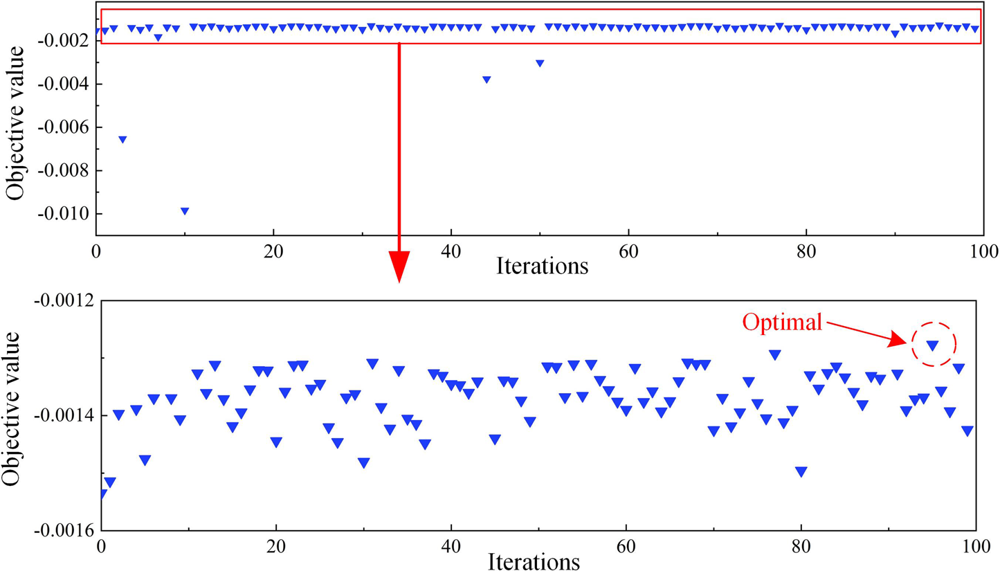
Optimizing process of the BO-XGBoost model.
TABLE 3
| Optimization method |
Hyperparameter | Search space |
Optimal value |
Number of iterations |
Optimal NMSE |
Time consumption |
|---|---|---|---|---|---|---|
| BO | n_estimators | [5, 500] | 384 | 100 | −0.00128 | 81 s |
| max_depth | [1, 50] | 43 | ||||
| learning_rate | [0.001, 0.3] | 0.1476 | ||||
| subsample | [0.6, 0.9] | 0.7811 | ||||
| GS | n_estimators | [5, 500] | 500 | 5,808 | −0.00181 | 5,196 s |
| max_depth | [1, 50] | 5 | ||||
| learning_rate | [0.001, 0.3] | 0.09 | ||||
| subsample | [0.6, 0.9] | 0.8 |
The optimal hyperparameters of the XGBoost model.
As shown in Table 3, during the optimization of the four hyperparameters of the XGBoost model, the BO algorithm achieved an optimal NMSE of −0.00128 in 81 s. In contrast, the GS algorithm required 5,196 s to achieve an optimal NMSE of −0.00181. Within the same search space, the BO algorithm demonstrated superior optimization performance, with a time consumption that was only 1.6% of that of the GS algorithm. This underscores the high efficiency of the BO algorithm.
4.2 Result analysis
The BO-XGBoost model, constructed with the optimal hyperparameter combination obtained through BO, is presented in Figure 6, illustrating its predictive results on both the training and test sets, with corresponding prediction errors shown in Figure 7. The model’s predictive performance is assessed using four metrics: the coefficient of determination R2, root mean square error (RMSE), mean absolute error (MAE), and mean absolute percentage error (MAPE). The method for calculating these metrics are referenced from the literature (Li et al., 2023; Wang et al., 2023; An et al., 2024a). As depicted in Figure 6, the BO-XGBoost model achieves R2 values of 0.99995 and 0.97551 on the training and test sets, respectively, indicative of exceptionally high predictive accuracy across both datasets. The MAE and MAPE of the BO-XGBoost model on the test set are 3.2940% and 4.51%, respectively. These minimal prediction errors suggest that the model is capable of accurately forecasting water inrush volumes in real-world tunnel engineering scenarios, thereby assisting managers in making informed decisions to prevent tunnel water inrush disasters and ensure the safe and efficient progression of tunnel construction.
FIGURE 6

Prediction results of the BO-XGBoost model: (a) training set; (b) test set.
FIGURE 7

Prediction error of the test set of BO-XGBoost model.
4.3 Model explanation
ML models are capable of accurately capturing the complex nonlinear relationships of input features; however, their “black-box” nature can undermine the persuasiveness of their predictive outcomes. To address this, the current study employs the SHAP method to interpret the BO-XGBoost model, thereby enhancing the credibility of its predictive results. Figure 8a illustrates the impact of each data sample involved in the interpretation on the model’s output, with red points indicating samples with low feature values and blue points representing samples with high feature values. It is evident from Figure 8a that h (groundwater level) and W (water-producing characteristics of the aquifer) exert a significant influence on the model’s output. Specifically, for groundwater level and the water-producing characteristics of the aquifer, samples with low feature values exhibit negative SHAP values. This suggests that a lower groundwater level and weaker water-producing characteristics of the aquifer are associated with a reduced volume of water inflow in the tunnel. Figure 8b presents the average SHAP values of each input feature across all sample data; the larger the average SHAP value, the more critical the feature is to the model. The average SHAP values for h, W, H, and RQD are 0.06, 0.05, 0.02, and 0.02, respectively. Consequently, the feature importance ranking for the BO-XGBoost model constructed in this study is h > W > H > RQD.
FIGURE 8

BO-XGBoost model explanation: (a) SHAP values of the input features; (b) importance of the input features.
The groundwater level (h) is the most critical feature, as it directly influences the magnitude of inflow during tunnel construction. Higher groundwater levels imply greater hydraulic pressure and potentially larger inflows, making h the most important factor in the model. Water-producing characteristics (W) is the second most significant, as they directly determine the replenishment of groundwater, which in turn affects tunnel inflow. Tunnel burial depth (H) is relatively less significant, yet still substantial. Tunnel depth influences the geological conditions and hydraulic pressure at the tunnel site. Although its direct impact is smaller compared to groundwater level and aquifer characteristics, it remains an important factor that must be comprehensively considered in practical engineering applications. Rock mass quality index (RQD) is the least significant factor. While RQD reflects the integrity and stability of the rock mass and has a critical impact on tunnel structural safety, its influence on predicting inflow is relatively minor.
The utilization of the SHAP method to interpret the BO-XGBoost model not only enhances the credibility of its predictive results but also provides a valuable reference for management and decision-makers in formulating appropriate strategies for the prevention and control of tunnel water inflow.
5 Discussion
5.1 Comparison analysis of different models’ performance
To demonstrate the superiority of the BO-XGBoost model proposed in this study in predicting the tunnel water inrush dataset, a comparative analysis of its predictive performance is conducted against three widely used ML models: Support Vector Regression, Decision Tree, and Random Forest. The training processes for the SVR, DT, and RF models follows the data preprocessing and hyperparameter optimization methods described earlier. To be more specific, BO is adopted to tune the hyperparameters of the baseline models to ensure a fair comparison. The optimal hyperparameters of these baseline models are displayed in Tables 4–6. The predictive performance of the four models on the test set is summarized in Table 7 and illustrated in Figure 9.
TABLE 4
| Parameter | Range | Value or type | Iterations | NMSE | Time consumption (s) |
|---|---|---|---|---|---|
| Kernel function | — | “rbf” | 100 | −0.003383 | 45 |
| c | [0.001, 1,000] | 542.25 | |||
| γ | [0.001, 1,000] | 12.91 |
Optimization parameters and results of Bayesian optimized SVR (BO-SVR) model.
TABLE 5
| Parameter | Range | Value or type | Iterations | NMSE | Time consumption (s) |
|---|---|---|---|---|---|
| max_depth | [1, 50] | 41 | 100 | −0.0026 | 34 |
| max_leaf_nodes | [1, 200] | 138 | |||
| min_samples_split | [2, 20] | 11 | |||
| min_samples_leaf | [1, 20] | 1 |
Optimization parameters and results of Bayesian optimized DT (BO-DT) model.
TABLE 6
| Parameter | Range | Value or type | Iterations | NMSE | Time consumption (s) |
|---|---|---|---|---|---|
| n_estimators | [10, 1,000] | 164 | 100 | −0.0026 | 538 |
| max_depth | [1, 50] | 39 | |||
| max_samples_split | [2, 20] | 3 | |||
| min_samples_split | [1,20] | 1 |
Optimization parameters and results of Bayesian optimized RF (BO-RF) model.
TABLE 7
| Models | RMSE | MAE | MAPE | R2 |
|---|---|---|---|---|
| BO-XGBoost | 7.5603 | 3.2940 | 0.0451 | 0.9755 |
| BO-SVR | 22.6936 | 18.8917 | 0.3495 | 0.7794 |
| BO-DT | 17.3770 | 9.3210 | 0.1181 | 0.8706 |
| BO-RF | 11.0818 | 6.4310 | 0.0746 | 0.9474 |
Predicting performance of the four candidate models.
Note: The bold values represent the best performance metrics.
FIGURE 9

Predicting results on the test set: (a) BO-XGBoost model; (b) BO-SVR model; (c) BO-DT model; (d) BO-RF model.
In Table 7, the optimal values for the four predictive performance metrics are emphasized in boldface. Among the 4 ML models optimized via BO, the BO-XGBoost model achieves the smallest prediction error and the highest coefficient of determination on the test set. As depicted in Figure 8, the prediction results of all 4 ML models closely align with the line on the test set, with the BO-XGBoost model demonstrating the highest degree of conformity to the line. Figure 10 illustrates the Taylor diagram of the prediction performance of the four candidate ML models. It can be observed that BO-XGBoost model is the closest to the reference point, indicating that BO-XGBoost model holds the best prediction performance. Further, Figure 11 illustrates the probability distribution of prediction errors for the 4 ML models on the test set. It is evident from Figure 11 that the prediction error distribution curve of the BO-XGBoost model is the tallest and narrowest among the four models, indicating that its error distribution is the most concentrated, with error values being relatively smaller than those of the other three models. Based on the fitting of the predicted values and the distribution of prediction errors on the test set, the predictive performance of the models can be ranked as follows: BO-XGBoost > BO-RF > BO-DT > BO-SVR.
FIGURE 10

Taylor diagram of the four candidate models.
FIGURE 11

Predicting error of the four candidate models.
5.2 Ablation experiment of input features
This study identified the input features for the WI prediction model based on existing studies and engineering experience, and employed the SHAP method to analyze the importance of these input features. To further analyze the importance of each input feature on model prediction performance, ablation experiments on input features were conducted. To be more specific, each input feature was individually removed, and the model was trained using the remaining three input features. For each feature, the ablation experiment was repeated 100 times, with a different “random_state” used each time to control the division of the training and test sets, thereby eliminating the influence of random factors during dataset splitting on the experimental results. The results of the ablation experiments are shown in Figure 12.
FIGURE 12

Prediction results of ablation experiment: (a) RMSE; (b) MAE; (c) MAPE; (d) R2.
As shown in Figure 12, without removing any features, the average RMSE, MAE, and MAPE values from the 100 experimental runs were smaller than those obtained when one feature was removed. This indicates that deleting an input feature increases the model’s prediction error and reduces its prediction accuracy. When the input feature h was deleted, the model’s RMSE, MAE, and MAPE average values were the largest, indicating that deleting “h” had the greatest impact on the model’s prediction performance. When the RQD was deleted, the RMSE, MAE, and MAPE average values were the smallest, indicating that deleting RQD hold the least impact on the model’s prediction performance.
Therefore, based on the increase in model error, the importance of input features in terms of their impact on model prediction performance can be ranked as: h > W > H > RQD. This conclusion is consistent with the results derived from SHAP analysis.
5.3 Enhancement of SMOGN on model performance
The predictive accuracy of ML models is significantly influenced by the size and quality of the dataset. To enhance the accuracy of the tunnel water inrush prediction model, this study employs SMOGN for data augmentation. To verify the effectiveness of SMOGN data augmentation in improving the predictive accuracy of the BO-XGBoost model, a series of comparative experiments are designed. The BO-XGBoost model is trained using datasets obtained from various parameter combinations, and the predictive accuracy on the test set is evaluated using MAE as the metric, as illustrated in Figure 13.
FIGURE 13

Predicting errors of the BO-XGBoost model on different datasets.
The candidate datasets are categorized into five groups, with each group’s base data defined as follows: Group A consists of the complete part of the original dataset; Group B is generated by interpolating the original data using the 5-Nearest Neighbor Imputation (5NNI) method (interpolated using KNNI with K = 5); Group C uses the 10NNI method; Group D utilizes the 15NNI method; and Group E is generated by interpolating the original dataset using the MI method. Each group contained four datasets: (1) not processed with the SMOGN method, (2) processed with the SMOGN method with K = 5 neighbors, (3) processed with the SMOGN method with K = 10 neighbors, and (4) processed with the SMOGN method with K = 15 neighbors.
From Figure 13, it is evident that the BO-XGBoost models trained on the base datasets of the five groups exhibit the highest MAE on the test set within each group. In contrast, the BO-XGBoost models trained on the datasets processed with the SMOGN technique in each group shows a significant reduction in MAE on the test set compared to the base datasets. This outcome indicates that the SMOGN data augmentation technique effectively reduces the prediction error of the BO-XGBoost model on the test set, thereby enhancing its predictive accuracy. Among the five base datasets, the BO-XGBoost models trained on the base datasets obtained by KNNI interpolation in Groups B, C, and D have slightly lower MAE on the test set compared to Group A (without interpolation) and Group E (interpolated with the MI method). KNNI interpolation of missing data can marginally improve the predictive accuracy of the BO-XGBoost model, whereas the MI interpolation technique diminishes the predictive accuracy of the BO-XGBoost model. This result suggests that for the tunnel water inrush missing dataset utilized in this study, KNNI is more suitable than the MI method for imputing missing values to enhance the model’s predictive accuracy. Furthermore, among the 20 datasets involved in this experiment, the model trained using dataset 15NNI with SMOGN [15NNI-SMOGN (K = 5)] had the lowest MAE on the test set, indicating the highest predictive accuracy. Consequently, this study selected this dataset for training the BO-XGBoost model.
5.4 Comparative analysis with related works
The performance of different models in predicting water inflow in tunnels from the previous study is summarized in Table 8. The R2 is taken as the accuracy metric for comparison. The BO-XGBoost model established in this study shows high prediction accuracy compared to most of the ML models in the related studies, indicating that the proposed BO-XGBoost model is as reliable as the models in the previous studies. However, models like LSTM, DNN, and GEP show better performance than the proposed BO-XGBoost model, suggesting that the efforts are still needed to improve the prediction accuracy of the BO-XGBoost model in further study.
TABLE 8
| Literature | Model | Input | R2 | Database size |
|---|---|---|---|---|
| Samadi et al. (2025) | AO-BPNN | H, h, RQD, W | 0.8817 | 600 |
| AdaD-RNN | 0.9007 | |||
| AdaG-LSTM | 0.9410 | |||
| AdaG-GRU | 0.9514 | |||
| Stacking-ensemble | 0.9730 | |||
| ALFS-IC | 0.9507 | |||
| Zhou et al. (2023a) | RF | H, h, RQD, W | 0.8726 | 600 |
| Bagging | 0.8693 | |||
| AdaBoost | 0.8683 | |||
| HGBoosting | 0.8147 | |||
| GBRT | 0.8673 | |||
| Voting | 0.8634 | |||
| Stacking | 0.8712 | |||
| GWO-RF | 0.9290 | |||
| Mahmoodzadeh et al. (2023) | GEP | H, h, RQD, W | 0.9804 | 600 |
| Mahmoodzadeh et al. (2021b) | LSTM | H, h, RQD, W | 0.9866 | 600 |
| DNN | 0.9815 | |||
| KNN | 0.7665 | |||
| GPR | 0.9714 | |||
| SVR | 0.8554 | |||
| DT | 0.7210 | |||
| Li et al. (2017) | GPR | FC, WT, SD, W, PYP, H | 0.9397 | 24 |
| SVM | 0.9134 | |||
| ANN | 0.8331 | |||
| This study | BO-XGBoost | H, h, RQD, W | 0.9755 | 1,347 |
| BO-SVR | 0.7794 | |||
| BO-DT | 0.8797 | |||
| BO-RF | 0.9474 |
Summary of tunnel squeezing prediction performance of related studies.
Notes: FC, fracture condition; WT, water transmission; SD, spacing distance; PYP, pore water pressure.
It is worth noting that the BO-XGBoost model proposed in this study is a black-box model. On the other hand, GEP method (Mahmoodzadeh et al., 2023) can generate mathematical formulas for prediction, thereby offering a more transparent solution. However, in terms of handling complex nonlinear relationships, GEP may exhibit lower predictive accuracy compared to BO-XGBoost. Additionally, GEP requires manual adjustment of parameters, such as population size and the number of generations, and the generated formulas may become overly complex, resulting in higher computational costs, especially when dealing with large-scale datasets. In contrast, the BO-XGBoost method can automatically tune hyperparameters and demonstrates strong capabilities in handling large-scale data.
5.5 Implementing of the ML model in real-world tunnels
The proposed BO-XGBoost model demonstrates satisfactory predictive performance in the task of tunnel WI prediction. Furthermore, the constructed BO-XGBoost model can fully leverage its predictive potential when applied to real tunnel projects for water inflow prediction. Specifically, the tunnel water inflow prediction workflow consists of three critical steps, as illustrated in
Figure 14.
Step 1: Data collection. Conducting engineering geological investigations and groundwater condition assessments for the tunnel under consideration, and collecting relevant tunnel design and construction data to obtain the values of model input parameters.
Step 2: Data preprocessing. Interpolating missing values in the input parameters and performing data scaling to normalize the dataset.
Step 3: WI prediction: Inputting the scaled data into the well-trained BO-XGBoost model to predict the WI and subsequently reversing the scaling of the predicted results.
FIGURE 14

Workflow of WI prediction in real-world tunnels.
Both the data preprocessing and WI prediction steps can be implemented in Python language. Anaconda is one of the ideal platforms for coding and running. Referencing the predicted WI values, informed decisions regarding tunnel construction planning and safety measures can be made. The ML models utilized in this study have relatively low computational requirements, as a computer equipped with an i5 processor and 16 GB of RAM is sufficient to deploy the XGBoost model developed in this research. Given that the number of input parameters for the model is only four, the XGBoost model can yield the predicted WI results within 1 s. This rapid prediction speed is fully capable of meeting the practical needs of tunnel engineering projects and providing a fast and reliable reference for the development of WI disaster prevention plans.
5.6 Limitations
The proposed approach achieves precise WI prediction based on the partially miss dataset by data imputation and augmentation. Moreover, The SHAP method is adopted to reveal the contribution of input features, which is not considered in existing WI prediction research. However, there’re still some limitations to be further explored. Firstly, KNNI and MI are used to achieve data imputation. However, KNNI is sensitive to outliers, as imputations heavily depend on distance-based neighbor selection, while MI tends to be more complex compared to single imputation approaches. Therefore, a more robust and efficient imputation method is required. Secondly, the dataset after imputation and SMOGN are still imbalanced with a few high WI samples. The SMOGN adopted in this paper achieve data augmentation, but data balance still needs further effort. Moreover, divergence analysis is not considered after data augmentation. Thirdly, although the BO-XGBoost model can precisely predict the WI, a WI interval will provide more information and reference for the engineers, which needs further exploration. Fourthly, the feature selection in this study referred to relevant studies and engineering experience. However, advanced feature selection methods, such as SFS, with XGBoost and RF with an explainable ensemble model and subset regression is not considered (Nandi et al., 2024; Mondal et al., 2025; Nandi and Das, 2025).
6 Conclusion
Tunnel water inflow disasters present substantial challenges to the safe and efficient construction of tunnels, and the ability to predict water inflow prior to tunnel excavation is critical for ensuring the safety of both machinery and personnel. However, the prediction of tunnel WI is fraught with challenges due to the influence of multiple factors. In this study, the XGBoost model is utilized for predicting WI, with BO employed to fine-tune the hyperparameters of the XGBoost model, thereby enhancing its predictive capabilities. To maximize the utility of tunnel data, 654 sets of missing data are imputed and augmented using the KNNI and SMOGN technique, respectively, and the resultant comprehensive dataset is divided in an 8:2 ratio for training and test purposes. The following conclusions are drawn from this study.
(1) The constructed BO-XGBoost model exhibited exceptionally high predictive accuracy on both the training and test sets, with an RMSE of 7.5603, MAE of 3.2940, MAPE of 4.51%, and R2 of 0.9755 on the test set.
(2) Compared to the predictive performance of SVR, DT, and RF models, the BO-XGBoost model demonstrates the highest R2 values and the smallest prediction errors, with the most concentrated error distribution. Consequently, the performance ranking of the 4 ML models in predicting WI is BO-XGBoost > BO-RF > BO-DT > BO-SVR.
(3) Different imputation methods and SMOGN parameters resulted in varied datasets, which in turn led to differing predictive accuracies of the trained models. Among the 20 datasets examined in this study, the BO-XGBoost model trained with 15NNI-SMOGN (K = 5) achieved the lowest MAE on the test set, indicating the highest predictive accuracy.
(4) The BO-XGBoost model was interpreted using the SHAP method, yielding a feature importance ranking of h > W > H > RQD.
The proposed WI prediction method can be applied in practical tunnelling projects following a process of data collecting, data preprocessing and WI prediction. Future research can focus on two aspects: (1) Integrate the ML model with real-time monitoring systems to facilitate real-time prediction of WI into tunnels; (2) Collect more tunnel data from diverse geological settings, and applicate the ML model to tunnels of different geological settings to enhance the generalization performance of the ML model.
Statements
Data availability statement
The raw data supporting the conclusions of this article will be made available by the authors, without undue reservation.
Author contributions
SJ: Conceptualization, Data curation, Formal Analysis, Investigation, Methodology, Validation, Visualization, Writing – original draft. GO: Conceptualization, Funding acquisition, Methodology, Project administration, Supervision, Writing – review and editing. TP: Data curation, Formal Analysis, Investigation, Resources, Software, Validation, Writing – original draft. YW: Data curation, Formal Analysis, Methodology, Validation, Visualization, Writing – review and editing. QS: Data curation, Investigation, Software, Visualization, Writing – original draft. PG: Conceptualization, Methodology, Project administration, Resources, Validation, Writing – review and editing.
Funding
The author(s) declare that financial support was received for the research and/or publication of this article. This study was financially supported by Education Department of Hunan Province of China (24B0915).
Conflict of interest
Author TP was employed by Sinohydro Engineering BUREAU 15 Co., LTD. Author QS was employed by Sinohydro Engineering BUREAU 4 Co., LTD.
The remaining author(s) declare that the research was conducted in the absence of any commercial or financial relationships that could be construed as a potential conflict of interest.
Generative AI statement
The author(s) declare that no Generative AI was used in the creation of this manuscript.
Publisher’s note
All claims expressed in this article are solely those of the authors and do not necessarily represent those of their affiliated organizations, or those of the publisher, the editors and the reviewers. Any product that may be evaluated in this article, or claim that may be made by its manufacturer, is not guaranteed or endorsed by the publisher.
Supplementary material
The Supplementary Material for this article can be found online at: https://www.frontiersin.org/articles/10.3389/feart.2025.1590203/full#supplementary-material
References
1
An X. Luo H. Zheng F. Jiao Y. Qi J. Zhang Y. (2024a). Explainable deep learning-based dynamic prediction of surface settlement considering temporal characteristics during deep excavation. Appl. Soft Comput.167, 112273. 10.1016/j.asoc.2024.112273
2
An X. Zheng F. Jiao Y. Li Z. Zhang Y. He L. (2024b). Optimized machine learning models for predicting crown convergence of plateau mountain tunnels. Transp. Geotech.46, 101254. 10.1016/j.trgeo.2024.101254
3
Bergstra J. Bardenet R. Bengio Y. Kégl B. (2011). “Algorithms for hyper-parameter optimization,” in Advances in neural information processing systems (Curran Associates, Inc.).
4
Berkowitz B. (2002). Characterizing flow and transport in fractured geological media: a review. Adv. Water Resour.25, 861–884. 10.1016/S0309-1708(02)00042-8
5
Bo Y. Huang X. Pan Y. Feng Y. Deng P. Gao F. et al (2023). Robust model for tunnel squeezing using Bayesian optimized classifiers with partially missing database. Undergr. Space10, 91–117. 10.1016/j.undsp.2022.11.001
6
Chawla N. V. Bowyer K. W. Hall L. O. Kegelmeyer W. P. (2002). SMOTE: synthetic minority over-sampling technique. J. Artif. Intell. Res.16, 321–357. 10.1613/jair.953
7
Chen T. Guestrin C. (2016). “XGBoost: a scalable tree boosting system,” in Proceedings of the 22nd ACM SIGKDD international conference on knowledge discovery and data mining (New York, NY: Association for Computing Machinery), 785–794. 10.1145/2939672.2939785
8
Dablain D. Krawczyk B. Chawla N. V. (2023). DeepSMOTE: fusing deep learning and SMOTE for imbalanced data. IEEE T. Neur. Net. Lear.34, 6390–6404. 10.1109/TNNLS.2021.3136503
9
Deng Z. Zhu X. Cheng D. Zong M. Zhang S. (2016). Efficient KNN classification algorithm for big data. Neurocomputing195, 143–148. 10.1016/j.neucom.2015.08.112
10
Du L. Gao R. Suganthan P. N. Wang D. Z. W. (2022). Bayesian optimization based dynamic ensemble for time series forecasting. Inf. Sci.591, 155–175. 10.1016/j.ins.2022.01.010
11
Farhadian H. Katibeh H. (2017). New empirical model to evaluate groundwater flow into circular tunnel using multiple regression analysis. Int. J. Min. Sci. Techno.27, 415–421. 10.1016/j.ijmst.2017.03.005
12
Farhadian H. Nikvar-Hassani A. (2019). Water flow into tunnels in discontinuous rock: a short critical review of the analytical solution of the art. B. Eng. Geol. Environ.78, 3833–3849. 10.1007/s10064-018-1348-9
13
Feng P. Li C. Zhang S. Meng J. Long J. (2024). Integrating shipborne images with multichannel deep learning for landslide detection. J. Earth Sci.-China35, 296–300. 10.1007/s12583-023-1957-5
14
Feurer M. Hutter F. (2019). “Hyperparameter optimization,” in Automated machine learning: methods, systems, challenges. Editors HutterF.KotthoffL.VanschorenJ. (Cham. Switzerland: Springer International Publishing), 3–33. 10.1007/978-3-030-05318-5_1
15
Geng X. Wu S. Zhang Y. Sun J. Cheng H. Zhang Z. et al (2023). Developing hybrid XGBoost model integrated with entropy weight and Bayesian optimization for predicting tunnel squeezing intensity. Nat. Hazards.119, 751–771. 10.1007/s11069-023-06137-0
16
Golian M. Teshnizi E. S. Nakhaei M. (2018). Prediction of water inflow to mechanized tunnels during tunnel-boring-machine advance using numerical simulation. Hydrogeol. J.26, 2827–2851. 10.1007/s10040-018-1835-x
17
Guan P. Ou G. Liang F. Luo W. Wang Q. Pei C. et al (2025). Tunnel squeezing prediction based on partially missing dataset and optimized machine learning models. Front. Earth Sci.13. 10.3389/feart.2025.1511413
18
Guo D. Li J. Li X. Li Z. Li P. Chen Z. (2022). Advance prediction of collapse for TBM tunneling using deep learning method. Eng. Geol.299, 106556. 10.1016/j.enggeo.2022.106556
19
He P. Xu F. Sun S. (2020). Nonlinear deformation prediction of tunnel surrounding rock with computational intelligence approaches. Geomat. Nat. Haz. Risk11, 414–427. 10.1080/19475705.2020.1729254
20
Holmøy K. H. Nilsen B. (2014). Significance of geological parameters for predicting water inflow in hard rock tunnels. Rock Mech. Rock Eng.47, 853–868. 10.1007/s00603-013-0384-9
21
Hou S. Liu Y. (2022). Early warning of tunnel collapse based on Adam-optimised long short-term memory network and TBM operation parameters. Eng. Appl. Artif. Intel.112, 104842. 10.1016/j.engappai.2022.104842
22
Huang X. Yin X. Liu B. Ding Z. Zhang C. Jing B. et al (2022). A gray Wolf optimization-based improved probabilistic neural network algorithm for surrounding rock squeezing classification in tunnel engineering. Front. Earth Sc-switz10. 10.3389/feart.2022.857463
23
Hutter F. Hoos H. H. Leyton-Brown K. (2011). “Sequential model-based optimization for general algorithm configuration,” in Learning and intelligent optimization. Editor CoelloC. A. C. (Berlin, Germany: Springer), 507–523. 10.1007/978-3-642-25566-3_40
24
Hwang J.-H. Lu C.-C. (2007). A semi-analytical method for analyzing the tunnel water inflow. Tunn. Undergr. Space. Technol.22, 39–46. 10.1016/j.tust.2006.03.003
25
Janković R. Mihajlović I. Štrbac N. Amelio A. (2021). Machine learning models for ecological footprint prediction based on energy parameters. Neural comput. Appl.33, 7073–7087. 10.1007/s00521-020-05476-4
26
Jin X. Li Y. Luo Y. Liu H. (2016). Prediction of city tunnel water inflow and its influence on overlain lakes in karst valley. Environ. Earth Sci.75, 1162. 10.1007/s12665-016-5949-y
27
Jong S. C. Ong D. E. L. Oh E. (2021). State-of-the-art review of geotechnical-driven artificial intelligence techniques in underground soil-structure interaction. Tunn. Undergr. Space. Technol.113, 103946. 10.1016/j.tust.2021.103946
28
Kim D. Pham K. Oh J.-Y. Lee S.-J. Choi H. (2022a). Classification of surface settlement levels induced by TBM driving in urban areas using random forest with data-driven feature selection. Autom. Constr.135, 104109. 10.1016/j.autcon.2021.104109
29
Kim J. Kim C. Kim G. Kim I. Abbas Q. Lee J. (2022b). Probabilistic tunnel collapse risk evaluation model using analytical hierarchy process (AHP) and Delphi survey technique. Tunn. Undergr. Space Technol.120, 104262. 10.1016/j.tust.2021.104262
30
Li S. He P. Li L. Shi S. Zhang Q. Zhang J. et al (2017). Gaussian process model of water inflow prediction in tunnel construction and its engineering applications. Tunn. Undergr. Space Technol.69, 155–161. 10.1016/j.tust.2017.06.018
31
Li S. C. Wu J. (2019). A multi-factor comprehensive risk assessment method of karst tunnels and its engineering application. B. Eng. Geol. Environ.78, 1761–1776. 10.1007/s10064-017-1214-1
32
Li X. Pan Y. Zhang L. Chen J. (2023). Dynamic and explainable deep learning-based risk prediction on adjacent building induced by deep excavation. Tunn. Undergr. Space Technol.140, 105243. 10.1016/j.tust.2023.105243
33
Liu D.-G. Yang Y. Mao C.-J. Wu J.-F. Wu J.-C. (2022). A comparative study on hydrodynamics and hydrochemistry coupled simulations of drainage pipe crystallization blockage in karst tunnels. J. Earth Sci.-China33, 1179–1189. 10.1007/s12583-022-1720-3
34
Mahmoodzadeh A. Ghafourian H. Hussein Mohammed A. Rezaei N. Hashim Ibrahim H. Rashidi S. (2023). Predicting tunnel water inflow using a machine learning-based solution to improve tunnel construction safety. Transp. Geotech.40, 100978. 10.1016/j.trgeo.2023.100978
35
Mahmoodzadeh A. Mohammadi M. Daraei A. Ali H. F. H. Abdullah A. I. Al-Salihi N. K. (2021a). Forecasting tunnel geology, construction time and costs using machine learning methods. Neural comput. Appl.33, 321–348. 10.1007/s00521-020-05006-2
36
Mahmoodzadeh A. Mohammadi M. Noori K. M. G. Khishe M. Ibrahim H. H. Ali H. F. H. et al (2021b). Presenting the best prediction model of water inflow into drill and blast tunnels among several machine learning techniques. Autom. Constr.127, 103719. 10.1016/j.autcon.2021.103719
37
Mirjalili S. Mirjalili S. M. Lewis A. (2014). Grey Wolf optimizer. Adv. Eng. Softw.69, 46–61. 10.1016/j.advengsoft.2013.12.007
38
Mondal S. Nandi B. Das S. (2025). Identifying optimal technique of reducing dimensionality of scour influencing hydraulic parameters applying SWOT analysis. Expert Syst. Appl.272, 126829. 10.1016/j.eswa.2025.126829
39
Nandi B. Das S. (2025). Predicting max scour depths near two-pier groups using ensemble machine-learning models and visualizing feature importance with partial dependence plots and SHAP. J. Comput. Civ. Eng.39, 04025007. 10.1061/JCCEE5.CPENG-6150
40
Nandi B. Patel G. Das S. (2024). Prediction of maximum scour depth at clear water conditions: multivariate and robust comparative analysis between empirical equations and machine learning approaches using extensive reference metadata. J. Environ. Manage.354, 120349. 10.1016/j.jenvman.2024.120349
41
Qi X. Wang H. Pan X. Chu J. Chiam K. (2021). Prediction of interfaces of geological formations using the multivariate adaptive regression spline method. Undergr. Space6, 252–266. 10.1016/j.undsp.2020.02.006
42
Samadi H. Mahmoodzadeh A. Elhag A. B. Alanazi A. Alqahtani A. Alsubai S. (2025). Application of hybrid-optimized and stacking-ensemble labeled neural networks to predict water inflow in drill-and-blast tunnels. Tunn. Undergr. Space Technol.156, 106273. 10.1016/j.tust.2024.106273
43
Shahriari B. Swersky K. Wang Z. Adams R. P. De Freitas N. (2016). Taking the human out of the loop: a review of bayesian optimization. Proc. IEEE104, 148–175. 10.1109/JPROC.2015.2494218
44
Sheini Dashtgoli D. Sadeghian R. Mahboubi Ardakani A. R. Mohammadnezhad H. Giustiniani M. Busetti M. et al (2024). Predictive modeling of shallow tunnel behavior: leveraging machine learning for maximum convergence displacement estimation. Transp. Geotech.47, 101284. 10.1016/j.trgeo.2024.101284
45
Song X. Y. Dao N. Branco P. (2022). “DistSMOGN: distributed SMOGN for imbalanced regression problems,” in Fourth international workshop on learning with imbalanced domains: theory and applications. Editors MonizN.BrancoP.TorgoL.JapkowiczN.WozniakM.WangS. (San Diego, CA: Jmlr-Journal Machine Learning Research), 183, 38–52.
46
Wang G. Fang Q. Du J. Wang J. Li Q. (2023). Deep learning-based prediction of steady surface settlement due to shield tunnelling. Autom. Constr.154, 105006. 10.1016/j.autcon.2023.105006
47
Wang X. Lai J. Qiu J. Xu W. Wang L. Luo Y. (2020). Geohazards, reflection and challenges in Mountain tunnel construction of China: a data collection from 2002 to 2018. Geomat. Nat. Haz. Risk11, 766–785. 10.1080/19475705.2020.1747554
48
Wen Z. Wang Q. Ma Y. Jacinthe P. A. Liu G. Li S. et al (2024). Remote estimates of suspended particulate matter in global lakes using machine learning models. Int. Soil Water Conserv. Res.12, 200–216. 10.1016/j.iswcr.2023.07.002
49
Xu C. Cao B. T. Yuan Y. Meschke G. (2024). A multi-fidelity deep operator network (DeepONet) for fusing simulation and monitoring data: application to real-time settlement prediction during tunnel construction. Eng. Appl. Artif. Intel.133, 108156. 10.1016/j.engappai.2024.108156
50
Xu Z. Shi H. Lin P. Ma W. (2022). Intelligent on-site lithology identification based on deep learning of rock images and elemental data. IEEE Geosci. Remote Sens. Lett.19, 1–5. 10.1109/LGRS.2022.3179623
51
Yao B. Bai H. Zhang B. (2012). Numerical simulation on the risk of roof water inrush in Wuyang Coal Mine. Int. J. Min. Sci. Techno.22, 273–277. 10.1016/j.ijmst.2012.03.006
52
Zhang J. Li D. Wang Y. (2020a). Predicting tunnel squeezing using a hybrid classifier ensemble with incomplete data. B. Eng. Geol. Environ.79, 3245–3256. 10.1007/s10064-020-01747-5
53
Zhang N. Niu M. Wan F. Lu J. Wang Y. Yan X. et al (2024). Hazard prediction of water inrush in water-rich tunnels based on random forest algorithm. Appl. Sci.-Basel14, 867. 10.3390/app14020867
54
Zhang W. Wu C. Zhong H. Li Y. Wang L. (2021). Prediction of undrained shear strength using extreme gradient boosting and random forest based on Bayesian optimization. Geosci. Front.12, 469–477. 10.1016/j.gsf.2020.03.007
55
Zhang W. Zhang R. Wu C. Goh A. T. C. Lacasse S. Liu Z. et al (2020b). State-of-the-art review of soft computing applications in underground excavations. Geosci. Front.11, 1095–1106. 10.1016/j.gsf.2019.12.003
56
Zhong C. Li G. Meng Z. (2022). Beluga whale optimization: a novel nature-inspired metaheuristic algorithm. Knowl.-Based Syst.251, 109215. 10.1016/j.knosys.2022.109215
57
Zhou J. Zhang Y. Li C. Yong W. Qiu Y. Du K. et al (2023a). Enhancing the performance of tunnel water inflow prediction using Random Forest optimized by Grey Wolf Optimizer. Earth Sci. Inf.16, 2405–2420. 10.1007/s12145-023-01042-3
58
Zhou J. Zhu S. Qiu Y. Armaghani D. J. Zhou A. Yong W. (2022). Predicting tunnel squeezing using support vector machine optimized by whale optimization algorithm. Acta Geotech.17, 1343–1366. 10.1007/s11440-022-01450-7
59
Zhou X. Zhao C. Bian X. (2023b). Prediction of maximum ground surface settlement induced by shield tunneling using XGBoost algorithm with golden-sine seagull optimization. Comput. Geotech.154, 105156. 10.1016/j.compgeo.2022.105156
60
Zhu X. Chu J. Wang K. Wu S. Yan W. Chiam K. (2021). Prediction of rockhead using a hybrid N-XGBoost machine learning framework. J. Rock Mech. Geotech.13, 1231–1245. 10.1016/j.jrmge.2021.06.012
Summary
Keywords
tunnel water inflow, XGBoost, bayesian optimization, data augmentation, model interpretation
Citation
Ju S, Ou G, Peng T, Wang Y, Song Q and Guan P (2025) Tunnel water inflow prediction using explainable machine learning and augmented partially missing dataset. Front. Earth Sci. 13:1590203. doi: 10.3389/feart.2025.1590203
Received
09 March 2025
Accepted
08 April 2025
Published
25 April 2025
Volume
13 - 2025
Edited by
Chong Xu, Ministry of Emergency Management, China
Reviewed by
Guoyang Liu, Shenyang University of Technology, China
Buddhadev Nandi, Jadavpur University, India
Wenkun Yang, Hohai University, China
Dayou Luo, Iowa State University, United States
Asmare Molla Reta, National Taiwan University of Science and Technology, Taiwan
Updates
Copyright
© 2025 Ju, Ou, Peng, Wang, Song and Guan.
This is an open-access article distributed under the terms of the Creative Commons Attribution License (CC BY). The use, distribution or reproduction in other forums is permitted, provided the original author(s) and the copyright owner(s) are credited and that the original publication in this journal is cited, in accordance with accepted academic practice. No use, distribution or reproduction is permitted which does not comply with these terms.
*Correspondence: Guangzhao Ou, ouguangzhao@hufe.edu.cn
Disclaimer
All claims expressed in this article are solely those of the authors and do not necessarily represent those of their affiliated organizations, or those of the publisher, the editors and the reviewers. Any product that may be evaluated in this article or claim that may be made by its manufacturer is not guaranteed or endorsed by the publisher.