Bayesian Hierarchical Models can Infer Interpretable Predictions of Leaf Area Index From Heterogeneous Datasets

Stojanović, Olivera; Siegmann, Bastian; Jarmer, Thomas; Pipa, Gordon; Leugering, Johannes

doi:10.3389/fenvs.2021.780814

METHODS article

Front. Environ. Sci., 11 January 2022

Sec. Environmental Informatics and Remote Sensing

Volume 9 - 2021 | https://doi.org/10.3389/fenvs.2021.780814

Bayesian Hierarchical Models can Infer Interpretable Predictions of Leaf Area Index From Heterogeneous Datasets

¹Neuroinformatics Lab, Institute of Cognitive Science, University of Osnabrück, Osnabrück, Germany
²Institute of Bio- and Geosciences, Plant Sciences (IBG-2), Jülich Research Centre, Jülich, Germany
³Working Group Remote Sensing and Digital Image Analysis, Institute of Computer Science, University of Osnabrück, Osnabrück, Germany

Environmental scientists often face the challenge of predicting a complex phenomenon from a heterogeneous collection of datasets that exhibit systematic differences. Accounting for these differences usually requires including additional parameters in the predictive models, which increases the probability of overfitting, particularly on small datasets. We investigate how Bayesian hierarchical models can help mitigate this problem by allowing the practitioner to incorporate information about the structure of the dataset explicitly. To this end, we look at a typical application in remote sensing: the estimation of leaf area index of white winter wheat, an important indicator for agronomical modeling, using measurements of reflectance spectra collected at different locations and growth stages. Since the insights gained from such a model could be used to inform policy or business decisions, the interpretability of the model is a primary concern. We, therefore, focus on models that capture the association between leaf area index and the spectral reflectance at various wavelengths by spline-based kernel functions, which can be visually inspected and analyzed. We compare models with three different levels of hierarchy: a non-hierarchical baseline model, a model with hierarchical bias parameter, and a model in which bias and kernel parameters are hierarchically structured. We analyze them using Markov Chain Monte Carlo sampling diagnostics and an intervention-based measure of feature importance. The improved robustness and interpretability of this approach show that Bayesian hierarchical models are a versatile tool for the prediction of leaf area index, particularly in scenarios where the available data sources are heterogeneous.

1 Introduction

The leaf area index (LAI) is a unitless measure (m² m⁻²) of the one-sided leaf surface area of a plant relative to the soil surface area (Watson, 1947). It characterizes, among other variables, the photosynthetic performance of plants (Watson, 1947; Chen and Black, 1992; Montheith and Unsworth, 2007), the size and density of the crop’s canopy and thus serves as an important indicator for the plant’s growth stage and stand productivity (Schueller, 1992; Cox, 2002; Bréda, 2003; Mulla, 2013; Yan et al., 2019). It plays a major role in meteorological, ecological, and agronomical modeling (Moran et al., 1995; Broge and Mortensen, 2002; Kergoat et al., 2002; Asner et al., 2003; Yan et al., 2012; Anita et al., 2014), as well as for studying the influence of climate change on crop growth (Gao et al., 2005; Manea and Leishman, 2014).

Various non-destructive methods exist to measure or estimate LAI directly (Jonckheere et al., 2004), but they typically require taking a large number of manual measurements in the field. Since this is a laborious process and it can be difficult to control for confounding variables such as weather, alternative faster approaches to infer LAI from indirect measures, e.g., spectroscopy and (hyper-)spectral imaging, have been investigated (Liu et al., 2016; Din et al., 2017; Yan et al., 2019; He et al., 2020). A common approach makes use of vegetation indices (VIs), which can be computed from distinct wavebands of spectral measurements, to estimate LAI (Huete et al., 2002). These measures, while well understood and easy to calculate, have several limitations. For example, most of them are sensitive to more than one plant parameter (e.g., LAI and chlorophyll content) (Govaerts et al., 1999; Dorigo et al., 2007), and especially for wheat crops, the non-linear relationship between numerous VIs and the LAI can lead to saturation for moderate to high LAI values (LAI $>$ 3) (Serrano et al., 2000; Nguy-Robertson et al., 2014). We instead use a Bayesian, spline-based regression method that utilizes the entire hyperspectral reflectance measurement to predict LAI and provides uncertainty estimates over all model parameters.

However, the relationship between LAI and spectral reflectance is also affected by other factors, such as the crop type, phenology, Sun illumination, local micro-climate, the type of soil, or the amount of precipitation (Kjaer et al., 2016; Din et al., 2017), and it may vary throughout the life cycle of the crop. These effects can be included in spatio-temporal models of LAI (Mustafa et al., 2014; Seyednasrollah et al., 2018; Jin et al., 2019; Qiu et al., 2020; Ji et al., 2021), which can be applied to data from aerial or satellite surveillance. This has the potential to greatly simplify monitoring crop growth across large or remote areas (Sun et al., 2021; Wan et al., 2021; Zhang et al., 2021).

But the annotated training data required for such spatio-temporal models, i.e., matched measurements of reflectance spectra, ground-truth LAI, and potential confounding variables, is not available for every location and crop. For example, the data used in this study consists of distinct datasets of corresponding LAI measurements and reflectance spectra, each set acquired on a single field over a period of one or 2 days. In this situation, the amount of labeled training data that can be acquired is too limited to fit either a full spatio-temporal model or a separate model for each field and/or growth stage. It is possible, in principle, to train a single model that generalizes across these conditions by simply pooling multiple datasets that were acquired under different conditions (see (Siegmann and Jarmer, 2015), for example). However, since the association between each data point and the specific dataset it belongs to (and thus its location and time) is lost in the pooling process, such a model is likely to perform worse than a spatio-temporal model or a field- and growth-stage-specific model, given sufficient training data. Ideally, we would like to find a compromise between these two extremes, i.e., between a single model trained on the pooled data on the one hand and an independent model for each dataset, on the other hand, that allows us to generalize over all the available datasets yet makes specifically adjusted predictions for each dataset. To this end, we propose a hierarchical, parameter-efficient Bayesian model, which implicitly accounts for the influence of location and time by allowing the model parameters to vary across different datasets.

Bayesian hierarchical models similar to the one suggested here are especially appealing for environmental sciences (Britten et al., 2021), where they have seen increasingly widespread use. For example, several recent studies applied Bayesian hierarchical models to time series of multispectral satellite images in order to assess the effects of climate change through land surface phenology (Senf et al., 2017; Seyednasrollah et al., 2018; Qiu et al., 2020; Babcock et al., 2021) or other indicators such as Normalized Difference Vegetation Index (Wilson et al., 2011). A similar remote sensing approach has been used to predict LAI and its spatio-temporal evolution for bamboo (Xing et al., 2019) and other forests (Naithani et al., 2013; Schraik et al., 2019). For agronomical models of the LAI of food crops such as rice (Xu et al., 2019), Brazilian Cowpea (Soratto et al., 2020) or white winter wheat (Qu et al., 2008), local multispectral measurements are often used instead of–or in addition to–satellite images. In most of these studies, Bayesian hierarchical models are used to impose prior domain knowledge, combine multimodal data sources, and integrate data collected at multiple resolutions of space and/or time, all of which ultimately improve prediction performance. By contrast, our primary goal is to show how Bayesian hierarchical models and associated tools can be used to construct and diagnose simple and interpretable models for heterogeneous datasets, which commonly occur in environmental sciences.

Based on these considerations, we develop a Bayesian hierarchical model according to the following steps: 1) we filter the spectral measurements to remove noise, 2) apply basis splines with adaptively placed knots to extract features from the spectra, 3) train a Bayesian hierarchical model to predict LAI from these features on labeled data, 4) select and validate the best performing model, 5) and estimate the importance of the individual features for prediction. Our model learns an easily interpretable general relationship between reflectance spectra and LAI, as well as the dataset-specific deviations from that baseline. By using a variant of Markov Chain Monte Carlo (MCMC) sampling, we can incorporate domain knowledge or regularization through prior distributions of the parameters and provide a full posterior probability distribution over these parameters, which allows the quantification of uncertainty. We compare two variants of this hierarchical approach with a non-hierarchical alternative and find that it indeed offers a favorable trade-off between prediction accuracy and model complexity.

2 Methods

2.1 The Dataset

We evaluate our proposed model on a combination of four datasets, totaling 191 pairs of measured reflectance spectra (see also Supplementary Figure S1 for examples) and corresponding measurements of the LAI on fields covered by white winter wheat (lat. Triticum aestivum).

Each pair of measurements was taken on a different square plot of size 50 cm×50 cm. The LAI values of each plot were measured multiple times in a non-destructive way and averaged to a single value per plot. Five reflectance spectra were acquired and averaged for each plot using a spectroradiometer from a height of 1.4 m above ground with a nadir view and converted to absolute reflectance values using a reflectance standard of known reflectivity (Spectralon, Labsphere Inc., United States). The data were collected on four different fields in different years, corresponding to different stages in the plants’ growth cycle, and there are minor differences in the data collection procedure.

The first two sampling areas, which we call Field A and Field B in the following, are located near Köthen, Germany, which is a part of one of the most important agricultural regions in Germany. The region is distinctly dry, with 430 mm mean annual precipitation due to its location in the Harz mountains. The mean annual temperature varies between 8◦C to 9 ◦C. The study area has an altitude of 70 m above sea level and is characterized by a Loess layer up to 1.2 m deep that covers a slightly undulated tertiary plain. The predominant soil types of the region are Chernozems, in conjunction with Cambisols and Luvisols. At two locations in this region, 57 spectral measurements were recorded on seventh to eighth May 2011 using two ASD FieldSpec III spectroradiometers (ASD Inc., United States) with 25° field of view optics. Another 74 measurements were taken on 24th to May 25, 2012, using one ASD FieldSpec III (ASD Inc., United States) and one SVC HR-1024 spectroradiometer (Spectra Vista Corporation, United States) with 14° field of view. For each location, the corresponding LAI was measured non-destructively with a SunScan device (Delta-T Devices Ltd., United States) in 2011 and an LAI 2000 (LI-COR Inc., United States) in 2012, and, respectively, five and four LAI measurements were averaged per plot. Data from this study area was also used and described in more detail in (Siegmann and Jarmer, 2015).

The other two sampling areas, called Field C and Field D in the following, are located near Demmin, Germany. The region has a mean annual precipitation of 550 mm, and a mean annual temperature of 8◦C. Albeluvisols interspersed by Haplic Luvisols dominate the sand-rich area. The observed area is south of the river Tollense, where the ground elevation drops from 70 m to 7 m due to glacial moraines causing high variability in soil conditions. At two locations in this region, 26 spectral measurements were recorded on, and another 34 on using SVC HR-1024i spectroradiometer (Spectra Vista Corporation, United States) in nadir view 1.4 m above the ground using 14° field of view optics. In this case, six measurements of LAI [taken with LAI 2000 (LI-COR Inc., United States)] were averaged for each plot.

The recorded spectra cover wavelengths in the range from 350 to 2,500 nm, of which we use the range from 400 to 1,350 nm (for details see Table 1). We preprocess these spectra by smoothing with a first-order Gaussian filter with width σ = 10 nm.

TABLE 1

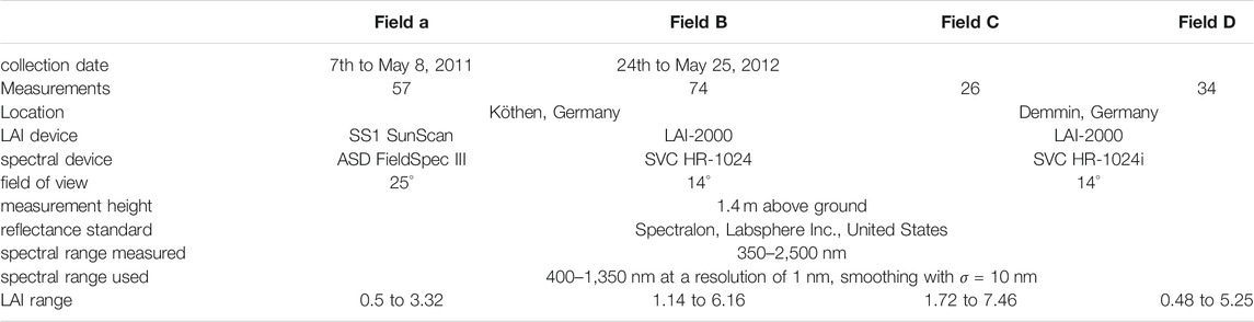
TABLE 1. Parameters of the dataset and the collection procedures.

For a summary of these parameters, see Table 1.

In the following, we reference specific subsets of this data. We introduce the following notation: all spectra-LAI-pairs for field j ∈ {1, …, 4} are numerically indexed by the set J^j, where J¹, J², J³, J⁴ correspond to the measurements from Field A, Field B, Field C, and Field D, respectively. We denote the ith ∈ J^j reflectance spectrum from dataset j by the function $R_{i}^{j} (λ)$ of the wavelength λ ∈ [400 nm, 1,350 nm], and the corresponding measured LAI value by $Y_{i}^{j}$ .

2.2 Feature Extraction From Reflectance Spectra With a Spline Basis

The data collection and preprocessing steps outlined above result in reflectance spectra of wavelengths 400–1,350 nm at a resolution of 1 nm. Since this representation is much too high dimensional for direct use, we extract the most important information into a low dimensional representation by computing the inner product between the preprocessed reflectance spectra and a set of eleven cubic basis splines (B-splines) with adaptively placed knots (see Figure 1).

FIGURE 1

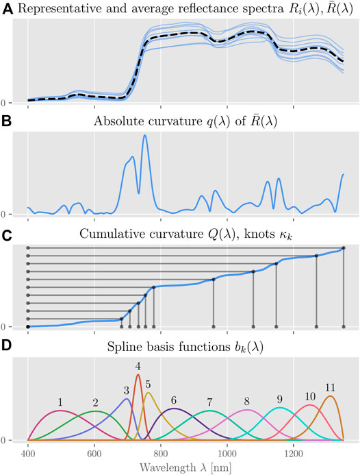
FIGURE 1. Adaptive knot-placement for B-Splines. (A) For the measured reflectance spectra R_i(λ), (B) we calculate the mean absolute curvature q(λ). (C) We then find knot positions such that the integral Q(λ) of this measure between any two successive knots κ_i, κ_i+1 is identical. (D) The result are 11 cubic spline basis functions b_k(λ) with non-uniformly spaced knots.

The positions κ_i, i ∈ {1, …, 11} of the inner knots, which determine the shape of the individual basis splines, are chosen such that the cumulative absolute curvature Q (κ_i+1) − Q (κ_i) of the average reflectance spectrum is equal between any two successive knots i and i + 1. We compute the absolute curvature q(λ) by convolving the average reflectance spectrum $\bar{R}$ with the second derivative of the Gaussian function g, and then compute the absolute value thereof¹. Formally, we can express this as follows:

\begin{array}{l} g (λ) & = \frac{1 n m}{\sqrt{2 π} σ} \exp (- \frac{λ^{2}}{σ^{2}}), & σ = 10 n m \\ \bar{R} (λ) & = \frac{1}{\sum_{j = 1}^{4} | J^{j} |} \sum_{j = 1}^{4} \sum_{i \in J^{j}} R_{i}^{j} (λ) \\ q (λ) & = |(\bar{R} * g^{″}) (λ)| \\ Q (x) & = \int_{400 n m}^{x} q (λ) d λ & \forall x \in [400 n m, 1350 n m] \\ Q_{max} & = Q (1350 n m) \\ κ_{i} & = Q^{- 1} (\frac{i - 1}{10} Q_{max}) & \forall i \in {1, \dots, 11} \end{array}

The eleven basis functions b_k, k ∈ {1, …, 11} are generated from this knot vector κ using the standard Cox-DeBoor algorithm (Boor, 1978), where the multiplicity of the first and last knot is three, i.e., all basis functions go to zero at their respective start and end knots. The last basis function b₁₂, which originates at knot κ₁₀, is not used. This heuristic algorithm results in a proportionally larger number of knots, and thus higher spatial resolution, where the reflectance spectra have the largest absolute curvature and hence “have most structure”; see also (Pipa et al., 2012; Ferrer Arnau et al., 2013; Tjahjowidodo et al., 2015). For each of the data-subsets j ∈ {1, …, 4}, we can then compute our model’s feature or design matrix X^j using these basis functions b_k(λ):

{(X^{j})}_{i, k} = ⟨ R_{i}^{j}, b_{k} ⟩ = \int_{400 n m}^{1350 n m} R_{i}^{j} (λ) b_{k} (λ) d λ, \forall i \in J^{j}, k \in {1, \dots, 11} (1)

2.3 Bayesian Markov Chain Monte Carlo Regression for Predicting LAI

Our primary objective is to construct a simple, interpretable model that can reliably predict the LAI value of a wheat plot directly from a corresponding reflectance spectrum. We are additionally interested in analyzing the model’s confidence, how well it generalizes, and which features it relies on most to make a prediction. Since the total available data is limited and stems from four heterogeneous datasets, prior constraints are required to prevent overfitting.

In order to meet all of these requirements, we design three different (non-)hierarchical Bayesian generalized linear models (GLM) (McCullagh and Nelder, 1989; Gelman et al., 2013) of different complexity. For each of these, we infer a full posterior distribution over model parameters from training data and use this to provide a full posterior predictive distribution over LAI scores on testing data. To generate representative samples from these probability distributions, we use a specific type of Hamiltonian Monte Carlo sampling, namely No-U-Turn-Sampling (Hoffman and Gelman, 2014) (NUTS), as implemented by the probabilistic programming package pyMC3 (Salvatier et al., 2016).

2.3.1 Model 1: A Baseline Model With Pooled Data

As a baseline (see Figure 2), we construct a simple generalized linear model, which we apply to all of the datasets j ∈ {1, …4} together. This model merely pools all available data but does not account for any systematic differences that might exist between the individual datasets. We assume the logarithm of the observed LAI scores to be normally distributed around an affine linear predictor μ^j with deviation σ, which is a model parameter with log-normal prior. The predictor μ^j is computed by the matrix-vector product between the dataset’s feature matrix X^j and the model’s weight vector w = (w₁, …, w₁₁), plus an additional bias parameter b. Including the unknown deviation parameter σ, the model thus has a total of 13 free parameters to be inferred from data. The individual parameters w_k and b have normal priors with standard deviation 1 and 11, respectively, to allow the individual bias term to counteract the effect of all 11 weights, if necessary. The baseline model is described by Eq. 2.

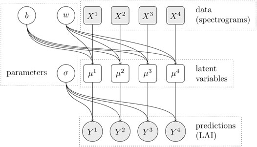
\begin{align} \log (σ) & \sim N o r m a l (0,1) \\ b & \sim N o r m a l (0,11) \\ w_{k} & \sim N o r m a l (0,1) & \forall k \in {1, \dots, 11} \\ μ^{j} & = X^{j} w + b, & \forall j \in {1, \dots, 4} \\ \log (Y_{i}^{j}) & \sim N o r m a l (μ_{i}^{j}, σ), & \forall j \in {1, \dots, 4}, i \in I^{j} \end{align} (2)

FIGURE 2

FIGURE 2. Dependency graph of the baseline model. For each dataset j (encoded in the feature matrix X^j and corresponding labels Y^j), the prediction depends on the same three shared parameters b, w and σ. Circles represent random variables, rectangles represent deterministic variables, filled shapes represent observed variables.

2.3.2 Model 2: A Model With Hierarchical Bias

Our second model (see Figure 3) extends the baseline model by an additional bias parameter b^j for each dataset and thus has a total of 17 free parameters. Due to the logarithmic link function, this additional parameter per dataset allows accounting for the overall variation in scale between the four different datasets. But rather than setting each parameter b^j independently (and thus adding three full degrees of freedom), we constrain them to be clustered around a common bias value b*, which replaces the bias term b in the baseline model. Therefore, the prior for the new variables b^j is a Normal distribution centered at b* with an order of magnitude smaller standard deviation of 11/10 = 1.1. The affine linear predictor μ^j then depends on the dataset-specific bias term b^j. The hierarchical bias model is described by Eq. 3.

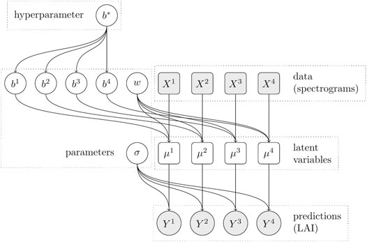
\begin{align} \log (σ) & \sim N o r m a l (0,1) \\ b^{*} & \sim N o r m a l (0,11) \\ b^{j} & \sim N o r m a l (b^{*}, 1.1) & \forall j \in {1, \dots, 4} \\ w_{k} & \sim N o r m a l (0,1) & \forall k \in {1, \dots, 11} \\ μ^{j} & = X^{j} w + b^{j}, & \forall j \in {1, \dots, 4} \\ \log (Y_{i}^{j}) & \sim N o r m a l (μ_{i}^{j}, σ), & \forall j \in {1, \dots, 4}, i \in I^{j} \end{align} (3)

FIGURE 3

FIGURE 3. Dependency graph of the hierarchical model with dataset-specific bias terms. The predictions for each dataset j depend on an individual bias parameter b^j, which in turn depends on the shared mean bias parameter b*.

2.3.3 Model 3: Full Hierarchical Model

Our third model (see Figure 4) extends the second model even further by also allowing the model weight vector w to vary for each dataset. Just like we did for the bias terms, we introduce the new parameter vectors w^j, and we constrain the individual parameters $w_{k}^{j}$ to be clustered around the corresponding common values $w_{k}^{*}$ with standard deviation 0.1. This increases the model’s degrees of freedom by an additional 44 parameters (11 for each dataset), resulting in a total of 61 free parameters. The affine linear predictor μ^j then depends on a dataset-specific weight vector w^j and a dataset-specific bias term b^j. The full hierarchical model is described by Eq. 4.

\begin{align} \log (σ) & \sim N o r m a l (0,1) \\ b^{*} & \sim N o r m a l (0,11) \\ b^{j} & \sim N o r m a l (b^{*}, 1.1) & \forall j \in {1, \dots, 4} \\ w_{k}^{*} & \sim N o r m a l (0,1) & \forall k \in {1, \dots, 11} \\ w_{k}^{j} & \sim N o r m a l (w_{k}^{*}, 0.1) & \forall k \in {1, \dots, 11}, j \in {1, \dots, 4} \\ μ^{j} & = X^{j} w^{j} + b^{j}, & \forall j \in {1, \dots, 4} \\ \log (Y_{i}^{j}) & \sim N o r m a l (μ_{i}^{j}, σ), & \forall j \in {1, \dots, 4}, i \in I^{j} \end{align} (4)

FIGURE 4

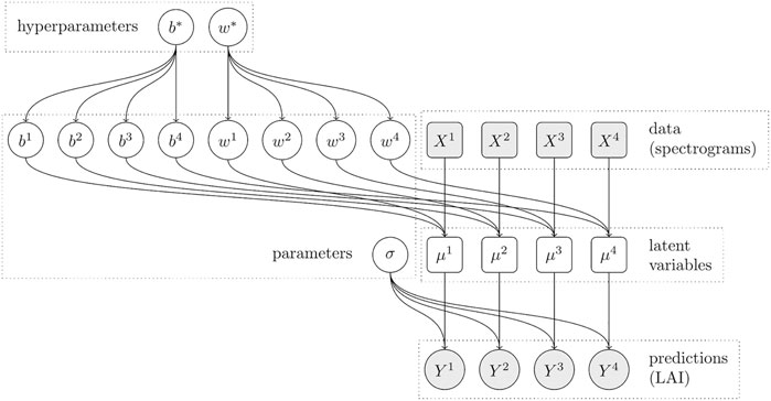
FIGURE 4. Dependency graph of the hierarchical model with dataset-specific bias and weight terms. The predictions for each dataset j now depend on an individual bias parameter b^j and weight vector w^j, which in turn depend on the shared bias parameter b* and the shared weight vector w*, respectively.

2.4 Model Selection Using Pareto-Smoothed Importance Sampling

To get an unbiased estimate of our model’s generalization error from the very limited available data, we would like to perform leave-one-out cross-validation (LOO-CV) and compute the expected log posterior predictive density (ELPD) for new data (Vehtari et al., 2019). Unfortunately, this is a prohibitively expensive computation when combined with MCMC sampling. However, the generated samples and their associated log-likelihood values contain sufficient information to estimate the LOO-CV ELPD by directly weighing the samples. This procedure is called Pareto-smoothed importance sampling (PSIS) (Vehtari et al., 2019). Combining these two methods, PSIS and LOO-CV, yields a validation method called PSIS-LOO-CV (Vehtari et al., 2019), which is beneficial in situations like this, where an MCMC sampling-based model is trained on a small dataset. As a result, we get for each model the ELPD score, which we use to compare the three proposed models, a parameter η, which can be interpreted as the effective number of degrees of freedom in the model, and the so-called Pareto shape parameters k_i, which assess for each data point i in the dataset, how much it affects the ELPD estimation. For data points where k_i exceeds 0.7, the PSIS-LOO-CV estimate becomes unreliable, which can also indicate an under-constrained model or an outlier in the data (Vehtari et al., 2019).

2.5 Evaluation of Feature Importance

To estimate the importance that our model assigns to each feature of the reflectance spectra, we calculate a model-agnostic measure of feature importance (Fisher et al., 2019) called model reliance (MR). Here, the importance of an individual feature is calculated as the relative change in the model’s error when the individual observations of only that feature are shuffled, compared to the error on non-shuffled data. This causal intervention intentionally breaks the dependence between different correlated features. Therefore, MR, unlike correlation analysis, is a causal tool to diagnose the model rather than the data. This is relevant here because the different features of our model are computed by taking the inner product between the reflectance spectra and a set of overlapping not independent basis functions and are hence certainly correlated. We use the same loss function as for the model selection, namely ELPD. Since this measure already estimates the logarithm of a quantity of interest (the posterior density), we use the difference between shuffled and non-shuffled ELPD instead of their ratio to estimate the logarithm of the MR for the posterior density. Because we are only interested in qualitatively ranking features by their importance, we normalize the resulting importance value of each feature by their average. To improve the robustness of this measure, the shuffling is repeated multiple times (here, ten times), and the results are averaged. Repeating this procedure for each feature of a model yields positive scores for ranking all features by their importance.

3 Results

In this section, we evaluate each of the three models presented above, namely the non-hierarchical model, the model with hierarchical bias term, and the full hierarchical model.

3.1 Model Predictions

First, we visualize the models’ accuracy and ability to generalize in a model-agnostic way by directly plotting predictions against the corresponding measured “ground-truth” values. For this purpose, we randomly select 80% of all available data (the training set, shown in blue) to infer model parameters, which we then use to predict the LAI for the remaining 20% of the data (the test set, shown in green). Due to the probabilistic nature of our models, a full posterior predictive distribution is given for each data point, which we summarize in Figure 5 (A),(C), and (E). We can observe that all three models make reasonable predictions, i.e., that the predicted LAI grows in proportion to the measured LAI. Because all our generalized linear models assume that the logarithms of the LAI scores are homoscedastic, the standard deviation of the predictive distribution increases with the measured LAI, as well. 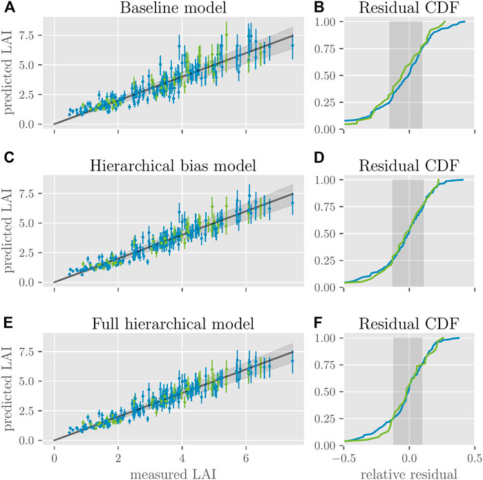Rather than the raw residuals $r_{i}^{j} = {\hat{Y}}_{i}^{j} - Y_{i}^{j}$ , we therefore compute the relative residuals ${\tilde{r}}_{i}^{j} = \frac{r_{i}^{j}}{Y_{i}^{j}}$ , each normalized by the corresponding measured LAI value $Y_{i}^{j}$ , and summarize them in the cumulative histograms shown in Figure 5 (B),(D) and (F). For all three models, the relative residuals are similar between training and test set, which indicates that they generalize well.

FIGURE 5

FIGURE 5. Model predictions of LAI. For the three models, (A), (C) and (E) plot for each data point (training data in blue and testing data in green) the predicted LAI values against the measured LAI values. Error bars indicate the interquartile range of the predictive distributions. Dots represent the expected value. The gray line shows the optimal predictions; the best 50% of model predictions lie within the gray cone around it. (B), (D), and (F) show the cumulative distribution function of the residuals, each normalized by the corresponding measured LAI value for training and testing data (blue and green lines). The gray areas show the same interquartile range as the cones in (A), (C), and (E).

3.2 Model Comparison

To quantify the generalization error of all three models more accurately, we use the PSIS-LOO-CV method on all available data to estimate the ELPD on novel data. This procedure yields several highly informative measures, which are summarized in Table 2. To verify the convergence of the sampling procedure for each model, we compare the marginal posterior distribution of each parameter across multiple chains and find no discrepancies or divergences (see also Supplementary Figures S2–S4). We can see that the highest ELPD (indicating the lowest generalization error) is achieved for the two hierarchical models, with little difference between them (−157.8 and −157.0, respectively, with a standard deviation of $\approx 11.5$ each). Suppose, for the sake of argument, that for a similar dataset, we would select models based purely on the ELPD. In that case, it might be a matter of chance to pick the model with only a hierarchical bias term (as in this case) or the full hierarchical model.

TABLE 2

TABLE 2. Comparison of the three models using PSIS-LOO-CV. The ELPD ± one standard deviation are listed for each model. #params denotes the number of parameters, η denotes the effective number of parameters. For each model, we show the number of data-points for which the Pareto shape parameter k falls into either of four different intervals.

However, due to the limited amount of training data and considering that the number of parameters ranges from 13 for the non-hierarchical baseline model to 17 for the model with hierarchical bias term to 61 for the full hierarchical model, we are also concerned with model complexity and the risk of overfitting. Since LOO-CV estimates generalization error directly, it does not need to explicitly penalize a large number of parameters, which is a significant advantage when comparing Bayesian hierarchical models. Instead, it allows us to estimate the model complexity of the three models by the so-called effective number of parameters η, which provides some intuition about how many degrees of freedom the model has to approximate the available data. As we see in Table 2, η = 13.3 is quite close to the parameter count of the non-hierarchical model on the pooled dataset. This only increases slightly to η = 15.0 for the hierarchical bias model, even though it has four additional parameters. However, adding another 44 parameters for the full hierarchical model increases η substantially to 24.9.

Since PSIS-LOO-CV emulates conventional LOO-CV, it provides additional information that can help us understand how prone each model is to overfitting: For each data point, the procedure yields the shape parameter k of a Pareto distribution, which indicates whether estimating the generalization error for that data point is reliable (k ∈ [ − ∞, 0.7], ideally k ≤ 0.5), potentially unreliable (k ∈ [0.7, 1]) or entirely unreliable (k ∈ [1, ∞])(Vehtari et al., 2019). As Table 2 shows, the full hierarchical model struggles with PSIS-LOO-CV for three data points, which may indicate that the model is more prone to overfitting to these potential “outliers” (see also Supplementary Figure S5).

As these numbers suggest, the model with a hierarchical bias term is the best choice because it is barely more complex than the non-hierarchical model, yet it performs at least as well as the full hierarchical model.

3.3 An Interpretable Kernel Function

As outlined above, all three models derive their predictions of LAI from a weighted linear combination of features, which we compute by taking inner products between the measured reflectance spectra and a set of B-spline basis functions. These linear operations can be equivalently expressed as taking the inner product between each reflectance spectrum and an inferred kernel function κ^j(λ), which provides a different, more interpretable perspective on the model.

To motivate this equivalent perspective, we look at how the reflectance spectra affect the linear predictors $μ_{i}^{j}$ of the respective GLMs in Eqs. 2–4, ignoring the contribution of the inferred bias terms here. For all three models², we can use Eq. 1 to rewrite the contribution of the features extracted from the ith reflectance spectrum $R_{i}^{j}$ of the jth dataset as follows:

\begin{align} μ_{i}^{j} - b^{j} & = \sum_{k} {(X^{j})}_{i, k} w_{k}^{j} \\ = \sum_{k} 〈 R_{i}^{j}, b_{k} 〉 w_{k}^{j} \\ = 〈 R_{i}^{j}, κ^{j} 〉 where κ^{j} (λ) = \sum_{k} w_{k}^{j} b_{k} (λ) \end{align} (5)

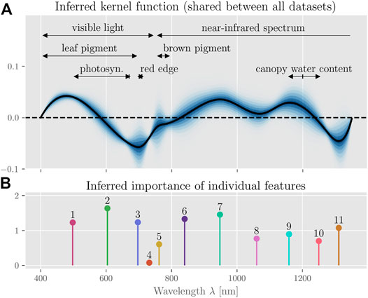
Since the parameters $w_{k}^{j}$ are random variables, the kernel functions κ^j are random variables, samples of which can be generated by combining the (static) basis functions b_k with samples of $w_{k}^{j}$ . Figure 6A shows the distribution of the inferred kernel function for our model of choice, i.e., the hierarchical bias model (for the other two models, see Supplementary Figures S6, S7). By analyzing this kernel function, we can identify regions of the reflectance spectrum that contribute positively or negatively (e.g., around λ ≈ 700 nm and λ ≈ 1,300 nm) to the predicted LAI score, and relate them to physical mechanisms.

FIGURE 6

FIGURE 6. Inferred kernel function and feature importance. (A) shows the posterior distribution of the inferred kernel function. The black line represents the expected kernel. We can relate several ranges of the reflectance spectrum to physical phenomena, namely effects due to green leaf pigment [400–700 nm (Cen and Borman, 1990; Aparicio et al., 2000)] and photosynthetic capacity [495–680 nm, peak at 670 nm (Cen and Borman, 1990; Aparicio et al., 2000; Weber et al., 2012)] and the red edge region [690–720 nm (Zhang et al., 2016)] in the visible light range, as well as the canopy’s water content [1,150 nm–1,260 nm (Sims and Gamon, 2003), peak absorption at around 1,200 nm (Weber et al., 2012; Wang C et al., 2017)] in the near-infrared range. (B) shows a stem-plot of the relative importance of each feature (enumerated; normalized by the average feature importance) as well as the resulting estimated importance of each wavelength.

3.4 Feature Importance

In addition to the sign and magnitude of each feature’s contribution (which are determined by the inferred weights; c. f. Supplementary Figures S2–S4), we are also interested in how important each individual feature is for the model’s prediction. We quantify this via MR as described above. Figure 6B shows that, except feature four, all features are indeed important for the prediction accuracy of the model. The low importance of feature four centered around 730 nm is likely due to the narrow domain of basis function b₄ (see Figure 1D), which indicates that this feature could be removed or an alternative knot-placement procedure could be chosen to reduce model complexity.

4 Discussion

Our results confirm that using a Bayesian hierarchical model not only leads to an improvement in the prediction accuracy over a non-hierarchical approach, but more importantly, it yields several qualitative benefits regarding interpretability, model complexity, and robustness.

One important benefit of the Bayesian hierarchical approach is that an appropriate choice of priors and model structure allows us to integrate additional model parameters without excessively increasing model complexity. For example, the number of spectral features used in our model directly determines the scale of the respective spline basis functions, which determines the resolution of our kernel function. This can create a trade-off between a model with lower spectral resolution and a model with a larger number of parameters. In the Bayesian approach, we can choose the model with more parameters without the risk of overfitting if we formalize our uncertainty and prior assumptions about the parameters appropriately. This is particularly important for hierarchical models, where we might want to add a large number of parameters to account for the specific variations in each subset of the data. Compare, for example, our full hierarchical model with its 61 parameters to the non-hierarchical baseline model with 13 parameters. Here, the addition of 48 new parameters only increases the effective degrees of freedom of the model by 11 and appears to increase the risk of overfitting only moderately. In our hierarchical bias model, we directly incorporate the fact that each of the four data subsets was recorded at a different growth stage of the plants, which affects the expected LAI, and hence requires a separate bias parameter. However, by simultaneously inferring the shared prior distribution over these separate parameters, we can ensure that the prediction on any one subset of the data benefits from the information contained in all the others. Of course, a non-hierarchical model can also benefit from heterogeneous data (see e.g. (Siegmann and Jarmer, 2015)), but it may fail in subtle ways if systematic differences between the data subsets obscure the relevant associations within each dataset³. In general, Bayesian hierarchical models allow us to conveniently include additional information about the dataset, domain knowledge, and regularizing priors, all of which can help to reduce the model’s effective degrees of freedom. For the often small and heterogeneous datasets used in environmental sciences (Britten et al., 2021), this can be a major advantage over alternative machine learning approaches such as Random Forest Regression (Houborg and McCabe, 2018; Srinet et al., 2019) or Deep Learning (Wang T et al., 2017; Apolo-Apolo et al., 2020; Yamaguchi et al., 2021), which may require prohibitive amounts of training data due to their typically large number of parameters.

We employ MCMC sampling to generate unbiased samples of the full posterior distributions over parameters and predictions, which allow us to use additional diagnostic tools and error measures. For example, we can directly estimate posterior densities, credible intervals, and even generalization errors via sample-based methods such as PSIS-LOO-CV, which are more broadly applicable than information criteria such as the Akaike Information Criterion (AIC), the Widely Applicable Information Criterion (WAIC), or the Bayesian Information Criterion (BIC) (Vehtari et al., 2017). In particular, we saw that a hierarchical model might have a considerably larger number of parameters with a comparatively minor increase in model complexity, making any form of regularization based directly on the number of parameters difficult. Besides better diagnostics, sample-based measures can also provide insights about the data itself, e.g., indicating which data points are potential “outliers” that the model is susceptible to (see Supplementary Figure S5).

In addition to descriptive statistics, we also estimate feature importance using an intervention-based model-agnostic method that artificially breaks the dependence between naturally correlated features. Thus, we can infer exactly which features the model relies on for its prediction–independently from the magnitude of the respective parameters. Such information can help domain experts identify potential problems, e.g,. if supposedly relevant features are ignored, or irrelevant features are relied on. This simple example shows how methods from causal analysis (Pearl, 2009) can help explain or interpret the model in qualitatively different ways than descriptive statistics alone.

Because we use a generalized linear model, we can additionally analyze and interpret the model’s linear predictor directly in the measurement space. Since the individual features are extracted from the spectra using B-spline basis functions, this linear predictor is just an inner product between a reflectance spectrum and a kernel function plus an additive bias term. Due to the logarithmic link function, the bias term ultimately has a scaling effect on the LAI predictions. The kernel function directly shows which wavelengths are associated with higher LAI, e.g., short wavelengths of the visible spectrum and much of the near-infrared spectrum, or lower LAI, e.g., around 600–750 nm. These results can be directly linked to physical phenomena and examined with domain knowledge. For example, the positive association for short wavelengths in the range 400–550 nm may be attributable to the effect of green leaf pigment, which reflects light in the range 400–700 nm (Cen and Borman, 1990; Aparicio et al., 2000). Similarly, the pronounced drop around the red edge (690–720 nm (Zhang et al., 2016)), which is related to the plants’ chlorophyll content (Richardson et al., 2002; Liu et al., 2004), total nitrogen (Cheng et al., 2005; Clevers and Kooistra, 2009) and yield (Huang et al., 2004; Rasooli Sharabiani et al., 2014), may be attributed to the plants’ photosynthetic capacity (495–680 nm (Cen and Borman, 1990; Aparicio et al., 2000; Weber et al., 2012)) that peaks at around 670 nm.

Finally, we opted for a simplistic, interpretable model of LAI as a function of spectral power, but the hierarchical Bayesian modeling approach makes it easy to extend the proposed model further. For a larger dataset, the model complexity could be increased, either by choosing broader priors or by increasing the number of parameters to improve its accuracy, or the additional measurements could be used to reduce the uncertainty over the model’s parameters. The data used in this study consists of measurements taken at four distinct locations and points in time. By allowing the specific parameters for each of these datasets to vary independently around a shared set of global parameters, we thus indirectly account for the combined effect of location and time. If a much larger number of datasets is used, their spatio-temporal distribution could also be taken into account explicitly, for example, by forcing the specific parameters of the datasets to be correlated, depending on their proximity in time and space, through an appropriate choice of a joint prior distribution. This approach leads to a full spatio-temporal model, which could also predict LAI on crop sites for which no training data is available. One could also include additional levels of hierarchy (e.g., to extend the model to other related plant species or different geographical regions), or other factors such as soil moisture content (Rad et al., 2011), the influence of climate change and CO2 concentration on crop growth (Gao et al., 2005; Manea and Leishman, 2014), the effects of warming asymmetry due to climate change (Cox et al., 2020), effects of microclimate (Hardwick et al., 2015), the influence of the amount of soil conditioner on the crops (Su et al., 2015), and ammonium level in the soil.

Data Availability Statement

The datasets generated for this study and the corresponding source code can be found online at: https://github.com/ostojanovic/bayesian_lai.

Author Contributions

OS and JL—Conceptualization, Methodology, Project administration, Software, Visualization, Writing—original draft; GP—Supervision, Resources, Conceptualization, Validation, Writing—review and editing; BS and TJ—Data curation, Conceptualization, Validation, Writing—review and editing.

Conflict of Interest

The authors declare that the research was conducted in the absence of any commercial or financial relationships that could be construed as a potential conflict of interest.

Publisher’s Note

All claims expressed in this article are solely those of the authors and do not necessarily represent those of their affiliated organizations, or those of the publisher, the editors and the reviewers. Any product that may be evaluated in this article, or claim that may be made by its manufacturer, is not guaranteed or endorsed by the publisher.

Acknowledgments

We would like to thank our reviewers for their detailed and constructive feedback, which helped to improve this manuscript.

Supplementary Material

The Supplementary Material for this article can be found online at: https://www.frontiersin.org/articles/10.3389/fenvs.2021.780814/full#supplementary-material

Footnotes

¹This is equivalent to computing the absolute curvature of the smoothed average reflectance spectrum $g * \bar{R}$ .

²To simplify notation, we write w^j and b^j for the (possibly) dataset-specific weight and bias terms, and set w^j = w or b^j = b for models that don’t make these dataset-specific distinctions

³In Supplementary Figure S6, we show that this is indeed the case here, as wavelength around 1,200 nm lead to a pronounced dip in the kernel function when data from multiple datasets is pooled, but this association disappears if the model is instead fit to any individual dataset. Looking at the pooled dataset, we would therefore be led to conclude that lower spectral power around 1,200 nm is a strong predictor of higher LAI. While this is correct on the artificially pooled dataset, it appears to be incorrect on any individual datasets. This may be an instance of Simpson’s paradox (Pearl, 2014), which suggests that a hierarchical model is more appropriate here

References

Anita, S. M., Richard, F., and Wang, S. (2014). Assessing the Impact of Leaf Area index on Evapotranspiration and Groundwater Recharge across a Shallow Water Region for Diverse Land Cover and Soil Properties. J. Water Res. Hydraulic Eng. 3, 60–73.

Google Scholar

Aparicio, N., Villegas, D., Casadesus, J., Araus, J. L., and Royo, C. (2000). Spectral Vegetation Indices as Nondestructive Tools for Determining Durum Wheat Yield. Agron. J. 92, 83–91. doi:10.2134/agronj2000.92183x