Experimental Observation of Dissolution Finger Growth in Radial Geometry

Reaction-infiltration instability refers to the morphological instability of a reactive fluid front flowing in a soluble porous medium. This process is important for many naturally occurring phenomena, such as the weathering and diagenesis of rocks, dissolution in salt deposits and melt extraction from the mantle. This paper is focused on experiments on dissolution finger growth in radial geometries in an analog fracture. In the experiments, pure water dissolves a plaster sample forming one of the fracture walls in a Hele-Shaw cell with controlled injection rate and aperture. The flow is directed inwards to the center, and we observe the reaction-infiltration instability developing along the relatively long perimeter of the plaster. Our experimental results show a number of features consistent with the theoretical and numerical predictions on the finger growth dynamics such as screening and selection between the fingers. Statistical properties of the dissolved part evolution with time are also investigated.

1. Introduction

In geological systems, dissolution plays an important role in the weathering and diagenesis of Earth's rocks [1, 2], chemical erosion of salt deposits [3, 4], and melt extraction from the mantle [5]. It is also of fundamental importance in many engineering applications, including dam stability [6] and CO₂ sequestration [7]. The important applications in the oil industry include acidization of petroleum reservoirs [8] in order to enhance oil and gas production by increasing the permeability of the rock [9, 10].

Because the reaction-infiltration instability plays an important role in a variety of fields, it stimulates dissolution-related research projects, both theoretical and numerical. Linear stability analysis can be applied to characterize the initial instability in porous media dissolution [11–14], but after fingering develops, we enter a nonlinear regime, where very few theoretical tools can be applied and one needs to resort to numerical simulations [3, 8, 15–21]. Compared to the theoretical and numerical works on the subject, there are relatively few experimental studies, especially on the observation of dissolution in quasi-2D radial geometry, which is the focus of this article.

In the lab experiments, two different setups are usually used: rock core acidization in Hassler cell and quasi-2D systems in Hele-Shaw cell which are aimed to study the dissolution in quasi-2D porous media and fractures. The number of core-flooding experiments reported in the literature is significantly larger than Hele-Shaw cell studies. There are two reasons for that: First, the core-flooding is closer to the real conditions encountered in the wellbore acidization in petroleum industry. Second, in core flooding it is easier to inject the flow into a porous matrix with negligible boundary effect. Many variables are systematically controlled in core-flooding experiments, including: injection rate [22], sample material [23], system scale [24], pH and temperature [25].

In this work, we have decided to use a 2D Hele-Shaw cell, as quasi-2D systems are easier to visualize and due to a large number of numerical work performed on these systems [18, 21, 26, 27]. On the experimental side, Daccord et al. [28, 29] investigated the water/plaster system in radial Hele-Shaw cell with central injection, and Golfier et al. [16] used a water/salt system in rectangular Hele-Shaw cells. The intention of both works was to study flow in a porous matrix, however, because of the difficulty in avoiding wall effects at boundaries, the injected water in most cases was found to flow along the difficult-to-detect aperture between the medium and the confining cell plate. This problem can be turned into advantage, if we promote it in a controlled manner instead of avoiding the wall flow. Such a controlled-aperture system can then be considered as an analog of a fracture, and the study is then directed at the investigation of how the fracture aperture evolves in time as a result of dissolution. Within this frame, Detwiler et al. [30] undertook a well-controlled dissolution study of the water/KDP system in rectangular Hele-Shaw cell and systematically measured the evolution of aperture at different flow rates. Osselin et al. [31] have performed experiments on the onset of reactive-infiltration instabilities in a fracture with a microfluidic setup using a rectangular water/plaster system. However, in many cases the relevant geometry is radial rather than rectangular, for instance, in the oil industry where the acid fluids are injected from a well, and in groundwater protection where pollutants expand with or without dissolution radially from the pollution source. Xu et al. [32] have recently studied dispersion in fractures in radial geometry with a dissolution pattern around the inlet.

The aim of this project is to study the dissolution finger growth in a fracture aperture of radial geometry. In section 2, we describe our experimental setup. In section 3, we present our experimental results discussing the screening effect and the statistical properties of the dissolved part evolution. The conclusions are drawn in section 4.

2. Description of Experiments

The experimental scheme is illustrated in Figure 1. A Hele-Shaw cell is formed by two circular glass plates which are separated by 1 mm aluminum spacers and held together by clamps. The bottom glass plate (diameter d₁ = 36.0 cm) is larger than the upper one (diameter d₂ = 25.0 cm) and has an external rim to hold the water surface at a fixed altitude level. There is an outlet at the center of the lower glass plate. A lightbox with a homogeneous intensity of light illuminates the system from below. A digital camera (Nikon D7100) records the sample images from the top every 5 min, and the whole dissolution process is thus recorded from the beginning of fluid withdrawing up to the dissolution channel breakthrough at the central outlet.

FIGURE 1

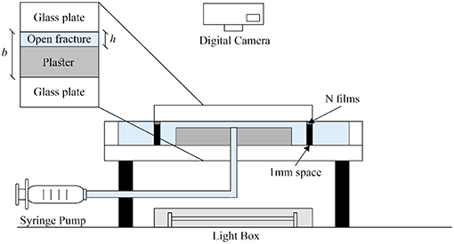
Figure 1. Schematic diagram of the experimental setup. A circular Hele-Shaw cell (spacing 1 mm) contains a plaster plate with a small gap h above the plaster upper surface. The aperture is created artificially by the spacers and kept clamped. Water is withdrawn by a syringe pump from the center of the bottom glass plate (the outlet), where it flows radially inwards. The plaster plate is surrounded by freshwater. The model is illuminated from below by a light box.

The circular plaster sample between the two plates was prepared as follows: A gypsum saturated water solution was first injected into the Hele-Shaw cell. We made a plaster paste by mixing water and plaster powder with the ratio 2:3 by weight. This paste was then injected from the center of the Hele-Shaw cell. The paste displaced the plaster saturated water and formed a circular plate of radius R₀ = 8.0cm. The hydration of this circular plaster paste requires approximately one hour to complete. During the plaster hydration process, the plaster paste was kept in the cell surrounded by saturated water. Over time, a form of segregation called bleeding takes place, where some of the water in the plaster tends to rise to the top surface of the plaster plate [33]. This process creates a small gap h₀ = 50μm above the upper surface of the plaster. After the completion of the hydration process, we removed the top glass plate, put several plastic films (each film thickness h₁ = 100μm) on the aluminum spacers and put back the top glass plate. The artificial aperture in our experiment h is defined as the distance between the upper glass plate and the surface of the plaster sample. The aperture created in this way is thus h = h₀ + n·h₁ where n is the number of plastic films. In the experiments reported here, we used n = 2 films which gave h = 250μm. When the sample preparation was completed, we started the dissolution experiments.

Because the radial dissolution by injection from the center gives a very short dissolution front around a point-like inlet, it becomes difficult to analyze the evolution of the fingers and the periodic wavelength from the experimental images in such a setup. Therefore, we chose instead to withdraw the water by a syringe pump from the outlet located at the center of the bottom glass plate. In this way, the freshwater flows from the rim toward the center and dissolves the plaster sample from the outer boundary. The instability can then be observed along the external perimeter of the sample. The withdrawing flow rate Q is set as Q = 0.18ml/min and the initial aperture of the artificial fracture is h = 250μm. The permeability of the porous plaster matrix is ${\kappa }_p=6.0·10^{-14}{m}^2$ [34] but the permeability of the fracture calculated as κ = h²/12 is around 5.2·10⁻⁹m², thus 5 magnitudes larger than the permeability of the porous matrix of our plaster sample. Therefore almost all the freshwater flows through the fracture instead of the porous matrix. The freshwater pumped through the system is distilled water at room temperature T = 22°C with pH = 7.17. The molecular diffusion coefficient of plaster (gypsum) in water is $D_m=1.0·10^{-9}{m}^2/s$ [35]. One experiment lasts around 10 days. The camera records the entire dynamic evolution process from initial instabilities to fingering formation, then to dissolution finger growth, and finally to the breakthrough of the longest fingers at the outlet.

2.1. Characteristic Timescales

The initial aperture h is an important characteristic length scale in our system. A characteristic timescale for diffusion across the aperture is $t_D=h^2/Dm=62.5s$ and the characteristic timescale for the reaction on the same length scale is t_R = h/k = 54.3s, where k is the chemical reaction kinetic constant (k = 4.6·10⁻⁶m/s) [36]. A relevant time scale for convection is the time it takes to flush the system, i.e., $t_C=\pi R_0^{2}h/Q=1,670s$. As we see, t_C ≫ t_D ≈ t_R. It means that reaction and diffusion across the aperture happen almost immediately compared with the time it takes for a fluid particle to flow through the system and we therefore expect that the calcium concentration of the water will reach the saturation concentration at the outlet. We performed density measurements to determine the concentration of the effluent solution. The concentration at the outlet is C_outlet = 2.5g/L which is consistent with the value of the saturation concentration reported in the literature C_sat = 2.53g/L [37].

3. Experimental Results and Discussion

3.1. Dissolution Finger Growth With Screening Effect

As the freshwater flows from the edge of the plaster sample to the center, the plaster begins to dissolve. In this process, the water becomes saturated, thus the dissolution concentrates at the perimeter. After several days, a visible dissolution front appears and it slowly develops into many dissolution fingers as a result of the reactive-infiltration instability. The further growth of these fingers becomes nonlinear, with scarce theoretical results concerning their shapes or growth rates [38, 39]. On the other hand, numerical models give a number of predictions for the fingering which can be qualitatively compared with experiments [17, 18, 21]. In particular, one can study the screening between the fingers, with the longer ones suppressing the growth of their shorter neighbors. As a results, approximately half of the active fingers continue to grow while the other half cease to grow. The process then repeats itself, leading to the scale-free distribution of finger lengths [40, 41].

Such a hierarchical growth of the fingers is clearly observed in the experimental images. Four experimental photos are chosen to show the process of the finger growth in Figure 2 (see also Figure S1 and Videos S1, S2).

FIGURE 2

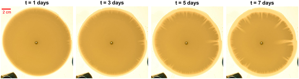
Figure 2. Experimental photos of the developing fingering pattern at different moments of time. The time interval between the photos is 2 days. In the circular plaster sample, the dark yellow disk is the undissolved part of plaster and the light yellow part represents the dissolved or partially dissolved part.

A dissolution front is extracted from the experimental images by using thresholding. A front position D is calculated as the distance between the point at the dissolution front and the outlet center. The front position varies with the polar angle θ and time t and we define the dissolution length as l(θ, t) = D(θ, t = 0)−D(θ, t), where D(θ, t = 0) is the initial front line. The initial front position D(θ, t = 0) has a small variation with the radius of the plaster sample R because in the experiments, the initial plaster sample is not perfectly circular. The dissolution length evolution with time l(θ, t) is shown in Figure 3. We should notice that the dissolution length function l(θ, t) is not a unique function because one polar angle θ could correspond to more than one dissolution front point, at different radial positions. This is because fingers develop along the radial direction and can also grow wider, with an orthoradial growth component.

FIGURE 3

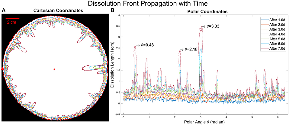
Figure 3. (A) Dissolution front propagation with time in Cartesian coordinates. The outermost red circle is the initial boundary, the red star marks the origin, where the outlet is located. The red arrow shows the point where θ = 0 and the direction in which the polar angle increases. Different colors of the curves show the dissolution front in different times with the time interval of 1 day between two neighboring curves. (B) The evolution of the dissolution length with time is shown in polar coordinates, obtained by calculating l(θ, t) = D(θ, t = 0)−D(θ, t) from binary experimental images. Different colors represent different times corresponding to the colors in (A). The longest finger located at θ = 3.03 radians and the two second longest fingers located at θ = 0.48 radians and θ = 2.18 radians are indicated in the plot.

In Figure 3, the competitive growth of the fingers is observed, due to the screening effect. The time interval we choose is fixed (1.0 day between neighboring curves), but the growth rate for different fingers varies significantly. One part of the fingering pattern (with θ in between 4 and 5 radians) grows more slowly than the rest over the entire time which means that the fluid flux through this part must have been significantly smaller. Such a flow inhomogeneity could be accidental, because the geometry of the system is not perfectly uniform. It leads to an initial circular symmetry breaking, where one side becomes a freshwater preferential flow path, screening off dissolution at other sides. Due to a positive feedback loop, eventually, some fingers will dominate so that most freshwater concentrates in these dissolution fingers. These long fingers then continue to grow while the short fingers grow very slowly (see Figure 3B). For the dissolution front propagation with time in a repeated experiment (see Figure S2). The longest fingers grow almost exponentially with time judging from Figure 4A, where we fit the finger length vs. time with an exponential function l = a·e^βt. The exponential growth rate β is shown in the legend of Figure 4A. Interestingly, the values of exponential growth rates are the same for all the three different fingers β = 0.32day⁻¹, which shows that the longest fingers grow largely independent of each other. From Figure 3A, the distance between these longest fingers is comparable to the length of their lengths. This is in agreement with the observation [41, 42] that the long finger screens the area of a lateral extent approximately equal to its length. For the analysis of the growth rates of other fingers (see Figure S3A).

FIGURE 4

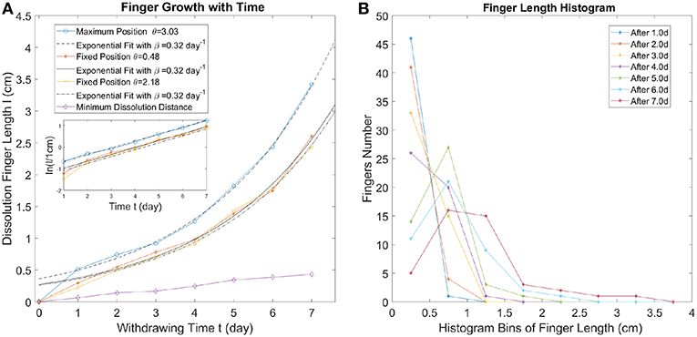
Figure 4. (A) The finger length evolution with time. The longest finger and two second longest fingers growth with time are displayed. Fingers located at different angular positions (see Figure 3B) are represented by different colors. The finger growth with time at these positions (fixed θ) have been fitted with an exponential function l = a·e^βt, displayed by three different black curves (solid or dashed). Minimum dissolution distance (corresponding to the point on the perimeter with the slowest dissolution speed) is shown by the purple curve. The inset shows the exponential fits for the finger length vs. time. (B) Dissolution finger length histograms obtained by counting the peaks in the dissolution length profiles (see Figure 3B). Different colors represent different times. The histogram bins cover the range 0–4.0 cm with bin size 0.5 cm.

In order to perform the statistical analysis of the dissolution finger growth, we find the local maxima of the curves in Figure 3B and define the dissolution finger length as the dissolution length corresponding to these maxima. The dissolution finger length histogram is shown in Figure 4B. The bins are chosen from 0 to 4.0 cm with a bin size of 0.5 cm, which divides the fingers into several types (orders). At an early stage, a lot of small fingers appear, with the length below 0.5 cm; these are the first order fingers. After 3 days, 2nd order fingers become clearly visible and the distribution gets wider as time progresses. With time, the number of small fingers (finger length below 1 cm in Figure 4B) decreases significantly since they are absorbed by the moving dissolution front while the longest fingers (finger length above 2.5 cm in Figure 4B) continue to grow. For the dissolution finger length histogram of other fingers (see Figure S3B).

3.2. Statistical Properties of the Dissolution Patterns

We observe from Figure 2 that the interface between the dissolved and the undissolved part is diffuse as the thickness of plaster sample at the dissolution front gradually transitions from the dissolved part to the undissolved part. Therefore, thresholding of the image, although useful for analyzing the dissolution patterns, leads inevitably to the information loss, as partially dissolved region are either interpreted as fully dissolved or as undissolved. In order to measure the aperture variation in the experimental images, a calibration between the thickness profile of the plaster sample and the intensity profile of the photos is performed by an X-ray Thickness Gauging REX-CELL 4X from Flow Capture [43–45].

The X-ray measurement for the thickness of dissolved plaster sample is displayed in Figure 5. The data records the photon counts at different positions of the sample by the X-ray measurement. Then the thickness profile is obtained from the intensity data by

$d=d_s·\frac{ln(I/I_0)}{ln(I_s/I_0)},$

where d_s is the initial thickness of the undissolved plaster sample, I is the intensity at a given pixel, I₀ is the average intensity value of the background and I_s is the average intensity value of the undissolved part. This formula is derived based on the Beer-Lambert law, $I=I_0{e}^{-\zeta d}$ [46] where ζ = 0.43mm⁻¹ normalized by a reference intensity $I_s=I_0{e}^{-\zeta d_s}$ corresponding to the undissolved sample.

FIGURE 5

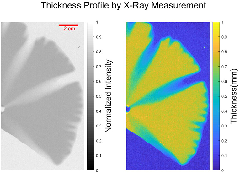
Figure 5. (Left) X-ray image of dissolved plaster sample captured by X-ray thickness gauge REX-CELL 4X from Flow Capture. The gray-scaled picture shown in the left panel is the normalized intensity of the X-ray measurement together with the color bar. (Right) Thickness profile of the dissolved plaster sample is displayed with the gradient-color picture together with the color bar.

The X-ray measurement and the calibration with the images illuminated by white light are shown in Figure 6. We compared the image illuminated by X-ray and the image illuminated by lightbox, we found a linear regression for the scatter plot of two images with y = 0.94·x−0.02. The Pearson correlation coefficient [47] between the two images is 0.95, which confirms that we can calculate the thickness of the plaster based on the lightbox measurements.

FIGURE 6

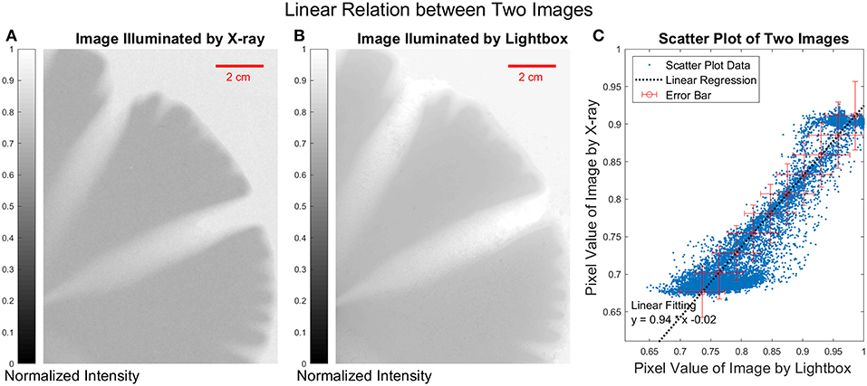
Figure 6. (A) X-ray image of the plaster sample. (B) Image illuminated by light box of the white light. (C) The scatter plot, each point in the scatter plot represents a pixel at the same position in both images illuminated by X-ray and the white light. The error bars are of the order of 5% on each of the axes. The pixel value below 0.7 represents the undissolved part and the pixel value above 0.9 represents the empty area outside of the plaster sample.

This allows us to quantify the local volume of dissolved gypsum in the sample. First, we define the aperture growth at a given point as as δh_t(r, θ) = h_t(r, θ) − h where h_t(r, θ) is the aperture at radial position r and polar angle θ and h is the initial aperture. Next, we calculate the dissolved volume per unit angle as $V_{\theta }(\theta ,t)={\int }_0^{R_0}\delta h_t(r)·rdr$. Note that the total dissolved volume is an integral of V_θ(θ, t) over the polar angle, $V_{diss}(t)={\int }_0^{2\pi }{V}_{\theta }(\theta ,t)d\theta$. Subsequently, we find it more convenient to use the arc length along the perimeter, p = R₀θ, instead of θ itself, to parameterize the experimental data. Then we define a local dissolved part as $S_D(p,t)={\int }_0^{R_0}\delta h_t(r)\frac{r}{R_0}dr=V_{\theta }(\theta ,t)/R_0$. The calculation method is illustrated in Figure 7.

FIGURE 7

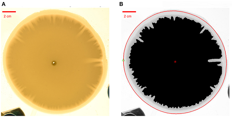
Figure 7. Estimation of the local dissolved part. (A) An experimental photo to be processed. (B) The red circular line acts as the reference curve, which represents the boundary of the initial plaster sample. The black part represents the undissolved part of the plaster sample. The red star marks the center of the plaster sample. We integrate the aperture variation values along a radial line from a point on the perimeter of the red circular line to the center.

The local dissolved part S_D(p, t) evolves in time as the dissolution front propagates, as illustrated in Figure 8A. In order to analyze this function quantitatively, a fast Fourier transform with a Blackman window [48] is applied at different times to obtain power spectrum S(k, t) where k is the spatial frequency or wavenumber (k = 1/λ where λ is the wavelength).

FIGURE 8

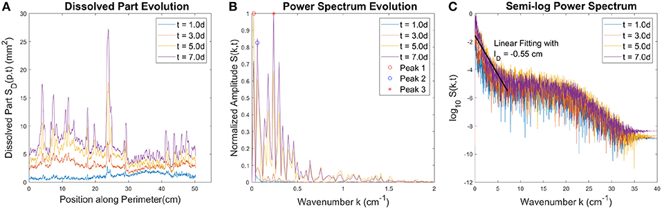
Figure 8. (A) The local dissolved part S_D(p, t) at different time moments. (B) The power spectrum of S_D(p, t) profiles presented in (A). Three main peaks are indicated in the plot. The first two (marked by red and blue circles) are related to the initial geometry of the plaster sample. On the other hand, the peak at 0.24 cm⁻¹ with wavelength ~4.2cm (marked by the red star) is related to the characteristic wavelength of the fingering pattern. (C) Semi-log plot of the power spectrum, which allows to observe power amplitude trends in a larger scope. The amplitude decays almost exponentially with wavenumber at low wavenumber (high wavelength), followed by a flat plateau at higher wavenumbers. The solid black line in (C) is the linear fit, the slope of which gives the characteristic decay length, l_D = 0.55cm.

The data in Figure 6A shows another manifestation of the screening of the shorter fingers by the longer ones. The power spectrum in Figure 8B has two main peaks before wavenumber k = 0.1cm⁻¹. The first peak (Peak 1 indicated by the red circle) at 0.02 cm⁻¹ with wavelength ~50cm comes from the perimeter of the plaster sample and the second peak (Peak 2 indicated by the blue circle) at 0.06 cm⁻¹ with a wavelength ~17cm is connected with the deviation of the initial gypsum disk from the circular shape (see Figures S6, S7 in Supplementary Data). We will ignore these two peaks because they come from the geometric properties of the initial plaster sample and not from the dissolution process. Beyond these two peaks, the maximum of the power spectrum is observed at 0.24cm⁻¹ with wavelength ~4.2cm, indicated by the red star in Figure 8B. This wavelength is related to the characteristic distance between the longest fingers, which is the main contribution to the power spectrum after finger formation. From the semi-log representation in Figure 8C, we see that the amplitude decays almost exponentially with wavenumber at low wavenumbers (high wavelengths), followed by a flat plateau at higher wavenumber. The decay is exponential, $S(k,t)\propto S(0,t)·e^{-l_D·k}$ with the characteristic decay length l_D = 0.55cm as shown in Figure 8C. The Fourier transform of a Lorentzian gives an exponential function [49]. The width of the Lorentzian gives the characteristic decay length of this exponential function. Since the largest fingers are of a similar shape, we expect the decay length l_D = 0.55cm to correspond to their characteristic width, which is indeed the case. The amplitude of the power spectrum decays gradually after a crossover at wavenumber k = 20cm⁻¹ corresponding to the wavelength λ = 0.5mm. The part of the spectrum with the wavenumber larger than k = 20cm⁻¹ are considered as noise from the roughness of the dissolution front.

The local dissolved part increases in time, as illustrated in Figure 9. The uncertainty of the measurement of the thickness variation is about 5% according to Figure 6. In Figure 9, we present the evolution of S_D(p, t) with error bars at several different points along the perimeter of the sample, the positions of which are marked by circles with the corresponding color in Figure 9A. Figure 9B further confirms the crucial role played in the dynamics by the competition between the fingers—the longer fingers speed up at the expense of the shorter ones.

FIGURE 9

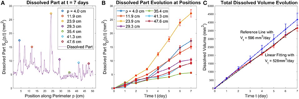
Figure 9. The left panel (A) shows the local dissolved part along the perimeter, S_D(p, t) at t = 7 days. The positions corresponding to the individual fingers, at p = [4.0, 11.9, 23.9, 29.3, 35.4, 41.3, 47.6] cm are marked with color circles. The center panel (B) displays the growth of S_D(p_i, t) at these positions with error bars. The right panel (C) shows the total dissolved volume as a function of time (red line) together with a linear fit (black line) and the theoretical estimate (blue line) with the corresponding error bars. The overlap between error bars show the experimental measurement fits well with the theoretical estimate.

To validate the calibration between the aperture profile and intensity profile, we have also calculated the growth of the total dissolved volume in time. The results, presented in Figure 9C, show that V_D increases linearly in time with the slope of 528mm³ per day. This is close to the theoretical estimate of the growth of the dissolved volume based on the mass balance of the reactant

$\begin{array}{ll}{V}_D=\frac{Q·c_{sat}}{{\rho }_b}t,& (1)\end{array}$

where Q is the injection rate, c_sat is the solubility of gypsum in pure water at 20°C and ρ_b is the bulk density of experimental plaster sample. For Q = 0.180ml/min, c_sat = 2.53g/l [37] and ρ_b = 1.1g/ml we get the rate of growth of the dissolved volume of 596mm³/day with an uncertainty of 9.1%, a reference line of this slope with error bars is shown in Figure 9C. The possible factors influencing the difference between the theoretical slope and the one measured experimentally come from inaccuracy in theH measurement of the bulk density ρ_b, measurement of the thickness variation δh and the linear fitting for V_D(t) based on the image analysis. Importantly, the second run of this experiment results in similar statistical properties of the dissolved pattern (see the Supplemental Data in Figures S4, S5).

We now introduce a calculation method by Vinningland et al. [50] who characterized the mean wavenumber of a growing interface. We again ignore the low frequencies since they are related to the initial geometric properties of the sample and only consider the wavelength λ < 10cm i.e., k > 0.1cm⁻¹. An average wavenumber < k > from the power spectrum S(k) for k > 0.1cm⁻¹ is defined as:

$\begin{array}{ll}<k>=\frac{\Sigma k·S(k)}{\Sigma S(k)},& (2)\end{array}$

where the sum Σ is over all k > 0.1cm⁻¹. The standard deviation σ_f is defined as:

$\begin{array}{ll}{\sigma }_k=\sqrt{\frac{\Sigma k^2·S(k)}{\Sigma S(k)}-<k{>}^2}.& (3)\end{array}$

We calculate the temporal evolution of < k > and σ_k, shown in Figure 10. As observed, the average wavenumber decreases with time, i.e. the average wavelength increases. This is another manifestation of the competition between the fingers: longer fingers develop and screen off nearby shorter fingers, which leads to a larger wavelength. The average wavenumber ranges from 0.4 to 1.8 cm⁻¹, thus the average wavelength ranges from 0.6 to 2.5 cm which fits the observation of characteristic wavelength from the experimental images.

FIGURE 10

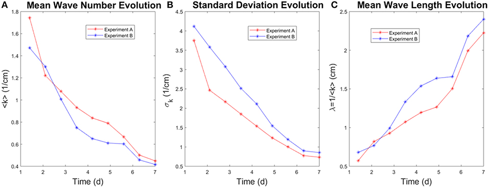
Figure 10. The figure shows the mean wavenumber (for k > 0.1cm⁻¹), its standard deviation and the mean wavelength (λ = 1/k) evolution with time for two experiments with the same aperture h = 250μm and the withdrawing rate Q = 0.18ml/min. (A) The average wavenumber decreases with time. (B) The standard deviation decreases with time. (C) The average fingering wavelength increases with time.

4. Conclusions

Understanding of the dissolution of fractures is important both for basic science (e.g., for studies of speleogenesis) as well as for technological applications, particularly in petroleum industry. However, the dissolution experiments in quasi-2d, radial geometry are relatively seldom performed. We dissolve a plaster disk in a Hele-Shaw cell by withdrawing water from the center, thus creating the inward flow pattern, and for the first time to our knowledge, we report the reactive-infiltration instability and finger growth along the perimeter of the circular plaster sample. The perimeter is 50.3 cm long which is sufficient to perform a statistical study of the reactive-infiltration instability and the dissolution fingers growth with time.

We observe strong competition between the growing fingers with the longest fingers growing exponentially with time in our experiments. We measure the thickness variation of the plaster sample by X-ray gauge and quantify the evolution in time of the dissolved volume. We then analyze it using statistical methods. The characteristic wavelength of the perturbations of the front is measured by a fast Fourier transform of the local dissolved volume. The power spectrum shows exponential decay with a characteristic decay length l_D = 0.55cm. On the other hand, the average wavelength increases linearly with time.

Our experimental setup allows us to adjust both the aperture thickness and flow rate. In the future, we will systematically control these two parameters to study a dissolution phase diagram in a radial geometry.

Data Availability

The raw data supporting the conclusions of this manuscript will be made available by the authors, without undue reservation, to any qualified researcher.

Author Contributions

LX and KM designed the experiment. LX performed the experiments, analyzed the data, and authored the paper. PS, RT, EF, and KM assisted with the interpretation and data analysis, and editing of the manuscript.

Funding

This project has received funding from the European Union's Seventh Framework Programme for research, technological development and demonstration under grant agreement no 316889. We acknowledge the support of the University of Oslo and the support by the Research Council of Norway through its Centres of Excellence funding scheme, project number 262644, the INSU ALEAS program, the French-Norwegian LIA D-FFRACT, and the support by the National Science Centre (Poland) under Research Grant 2012/07/E/ST3/01734.

Conflict of Interest Statement

The authors declare that the research was conducted in the absence of any commercial or financial relationships that could be construed as a potential conflict of interest.

Acknowledgments

We thank Atle Jensen, Bin Hu for technical support of X-ray measurement and Marcel Moura, Fredrik K. Eriksen, Mihailo Jankov, Monem Ayaz, Guillaume Dumazer, and Florian Osselin for useful discussions.

Supplementary Material

The Supplementary Material for this article can be found online at: https://www.frontiersin.org/articles/10.3389/fphy.2019.00096/full#supplementary-material

Video S1. The video of the experiment described in the main text shows the sequence of the experimental photos of the developing fingering pattern at different moments of time.

Video S2. The video of the experiment described in the Supplementary Material shows the sequence of the experimental photos of the developing fingering pattern at different moments of time.

References

1. Iyer K, Jamtveit B, Mathiesen J, Malthe-Sørenssen A, Feder J. Reaction-assisted hierarchical fracturing during serpentinization. Earth Planet Sc Lett. (2008) 267:503–16. doi: 10.1016/j.epsl.2007.11.060

CrossRef Full Text | Google Scholar

2. Ortoleva P, Chadam J, Merino E, Sen A. Geochemical self-organization II: the reactive-infiltration instability. Am J Sci. (1987) 287:1008–40. doi: 10.2475/ajs.287.10.1008

CrossRef Full Text | Google Scholar

3. Bekri S, Thovert J, Adler P. Dissolution of porous media. Chem Eng Sci. (1995) 50:2765–91. doi: 10.1016/0009-2509(95)00121-K

CrossRef Full Text | Google Scholar

4. Steefel CI, Lasaga AC. A coupled model for transport of multiple chemical species and kinetic precipitation/dissolution reactions with application to reactive flow in single phase hydrothermal systems. Am J Sci. (1994) 294:529–92. doi: 10.2475/ajs.294.5.529

CrossRef Full Text | Google Scholar

5. Aharonov E, Spiegelman M, Kelemen P. Three-dimensional flow and reaction in porous media: Implications for the Earth's mantle and sedimentary basins. J Geophys Res. (1997) 102:14821–14. doi: 10.1029/97JB00996

CrossRef Full Text | Google Scholar

6. Romanov D, Gabrovšek F, Dreybrodt W. Dam sites in soluble rocks: a model of increasing leakage by dissolutional widening of fractures beneath a dam. Eng Geol. (2003) 70:17–35. doi: 10.1016/S0013-7952(03)00073-5

CrossRef Full Text | Google Scholar

7. Michael K, Golab A, Shulakova V, Ennis-King J, Allinson G, Sharma S, et al. Geological storage of CO2 in saline aquifers review of the experience from existing storage operations. Int J Greenh Gas Con. (2010) 4:659–67. doi: 10.1016/j.ijggc.2009.12.011

CrossRef Full Text | Google Scholar

8. Fredd CN, Fogler HS. Influence of transport and reaction on wormhole formation in porous media. AIChE J. (1998) 44:1933–49. doi: 10.1002/aic.690440902

CrossRef Full Text | Google Scholar

9. Lake LW, Liang X, Edgar TF, Al-Yousef A, Sayarpour M, Weber D, et al. Optimization of oil production based on a capacitance model of production and injection rates. In: Hydrocarbon Economics and Evaluation Symposium. Dallas, TX: Society of Petroleum Engineers (2007).

Google Scholar

10. Sudaryanto B, Yortsos YC. Optimization of displacements in porous media using rate control. In: SPE Annual Technical Conference and Exhibition. New Orleans, LA: Society of Petroleum Engineers (2001).

Google Scholar

11. Chadam J, Hoff D, Merino E, Ortoleva P, Sen A. Reactive infiltration instabilities. IMA J Appl Math. (1986) 36:207–21. doi: 10.1093/imamat/36.3.207

CrossRef Full Text | Google Scholar

12. Szymczak P, Ladd AJ. Instabilities in the dissolution of a porous matrix. Geophys Res Lett. (2011) 38:L07403. doi: 10.1029/2011GL046720

CrossRef Full Text | Google Scholar

13. Szymczak P, Ladd AJ. Reactive-infiltration instabilities in rocks. Part 2. Dissolution of a porous matrix. J Fluid Mech. (2014) 738:591–630. doi: 10.1017/jfm.2013.586

CrossRef Full Text | Google Scholar

14. Szymczak P, Ladd AJ. Reactive-infiltration instabilities in rocks. Fracture dissolution. J Fluid Mech. (2012) 702:239–64. doi: 10.1017/jfm.2012.174

CrossRef Full Text | Google Scholar

15. Budek A, Szymczak P. Network models of dissolution of porous media. Phys Rev E. (2012) 86:056318. doi: 10.1103/PhysRevE.86.056318

PubMed Abstract | CrossRef Full Text | Google Scholar

16. Golfier F, Zarcone C, Bazin B, Lenormand R, Lasseux D, Quintard M. On the ability of a Darcy-scale model to capture wormhole formation during the dissolution of a porous medium. J Fluid Mech. (2002) 457:213–54. doi: 10.1017/S0022112002007735

CrossRef Full Text | Google Scholar

17. Kalia N, Balakotaiah V. Modeling and analysis of wormhole formation in reactive dissolution of carbonate rocks. Chem Eng Sci. (2007) 62:919–28. doi: 10.1016/j.ces.2006.10.021

CrossRef Full Text | Google Scholar

18. Panga MK, Ziauddin M, Balakotaiah V. Two-scale continuum model for simulation of wormholes in carbonate acidization. AIChE J. (2005) 51:3231–48. doi: 10.1002/aic.10574

CrossRef Full Text | Google Scholar

19. Zhang C, Kang Q, Wang X, Zilles JL, Muller RH, Werth CJ. Effects of pore-scale heterogeneity and transverse mixing on bacterial growth in porous media. Environ Sci Technol. (2010) 44:3085–92. doi: 10.1021/es903396h

PubMed Abstract | CrossRef Full Text | Google Scholar

20. Zhang X, Deeks LK, Glyn Bengough A, Crawford JW, Young IM. Determination of soil hydraulic conductivity with the lattice Boltzmann method and soil thin-section technique. J Hydrol. (2005) 306:59–70. doi: 10.1016/j.jhydrol.2004.08.039

CrossRef Full Text | Google Scholar

21. Szymczak P, Ladd A. Wormhole formation in dissolving fractures. J Geophys Res. (2009) 114:B06203. doi: 10.1029/2008JB006122

CrossRef Full Text | Google Scholar

22. Daccord G, Lenormand R. Fractal patterns from chemical dissolution. Nature. (1987) 325:41–3. doi: 10.1038/325041a0

CrossRef Full Text | Google Scholar

23. Hoefner M, Fogler HS. Pore evolution and channel formation during flow and reaction in porous media. AIChE J. (1988) 34:45–54. doi: 10.1002/aic.690340107

CrossRef Full Text | Google Scholar

24. McDuff D, Shuchart CE, Jackson S, Postl D, Brown JS. Understanding wormholes in carbonates: unprecedented experimental scale and 3-D visualization. In: SPE Annual Technical Conference and Exhibition. Florence: Society of Petroleum Engineers (2010).

Google Scholar

25. Wang Y, Hill A, Schechter R. The optimum injection rate for matrix acidizing of carbonate formations. In: SPE Annual Technical Conference and Exhibition. Houston, TX: Society of Petroleum Engineers (1993).

Google Scholar

26. Szymczak P, Ladd A. Microscopic simulations of fracture dissolution. Geophys Res Lett. (2004) 31:L23606. doi: 10.1029/2004GL021297

CrossRef Full Text | Google Scholar

27. Cohen C, Ding D, Quintard M, Bazin B. From pore scale to wellbore scale: impact of geometry on wormhole growth in carbonate acidization. Chem Eng Sci. (2008) 63:3088–99. doi: 10.1016/j.ces.2008.03.021

CrossRef Full Text | Google Scholar

28. Daccord G, Touboul E, Lenormand R. Chemical dissolution of a porous medium: limits of the fractal behaviour. Geoderma. (1989) 44:159–65. doi: 10.1016/0016-7061(89)90025-6

CrossRef Full Text | Google Scholar

29. Daccord G. Chemical dissolution of a porous medium by a reactive fluid. Phys Rev Lett. (1987) 58:479. doi: 10.1103/PhysRevLett.58.479

PubMed Abstract | CrossRef Full Text | Google Scholar

30. Detwiler RL, Glass RJ, Bourcier WL. Experimental observations of fracture dissolution: the role of Peclet number on evolving aperture variability. Geophys Res Lett. (2003) 30:1648. doi: 10.1029/2003GL017396

CrossRef Full Text | Google Scholar

31. Osselin F, Kondratiuk P, Budek A, Cybulski O, Garstecki P, Szymczak P. Microfluidic observation of the onset of reactive-infitration instability in an analog fracture. Geophys Res Lett. (2016) 43:6907–15. doi: 10.1002/2016GL069261

CrossRef Full Text | Google Scholar

32. Xu L, Marks B, Toussaint R, Flekkøy EG, Måløy KJ. Dispersion in fractures with ramified dissolution patterns. Front Phys. (2018) 6:29. doi: 10.3389/fphy.2018.00029

CrossRef Full Text | Google Scholar

33. Powers TC. The Properties of Fresh Concrete. New York, NY: John Wiley and Sons (1968).

Google Scholar

34. Ewers OR. Cavern Development in the Dimensions of Length and Breadth (Open access dissertations and thesis). McMaster University, Hamilton, ON, Canada (1982).

Google Scholar

35. Colombani J, Bert J. Holographic interferometry study of the dissolution and diffusion of gypsum in water. Geochim Cosmochim Acta. (2007) 71:1913–20. doi: 10.1016/j.gca.2007.01.012

CrossRef Full Text | Google Scholar

36. Colombani J. Measurement of the pure dissolution rate constant of a mineral in water. Geochim Cosmochim Acta. (2008) 72:5634–40. doi: 10.1016/j.gca.2008.09.007

CrossRef Full Text | Google Scholar

37. Klimchouk A. The dissolution and conversion of gypsum and anhydrite. Int J Speleol. (1996) 25:2. doi: 10.5038/1827-806X.25.3.2

CrossRef Full Text | Google Scholar

38. Nilson RH, Griffiths SK. Wormhole growth in soluble porous materials. Phys Rev Lett. (1990) 65:1583–6. doi: 10.1103/PhysRevLett.65.1583

PubMed Abstract | CrossRef Full Text | Google Scholar

39. Kondratiuk P, Szymczak P. Steadily translating parabolic dissolution fingers. SIAM J Appl Math. (2015) 75:2193–213. doi: 10.1137/151003751

CrossRef Full Text | Google Scholar

40. Huang Y, Ouillon G, Saleur H, Sornette D. Spontaneous generation of discrete scale invariance in growth models. Phys Rev E. (1997) 55:6433. doi: 10.1103/PhysRevE.55.6433

CrossRef Full Text | Google Scholar

41. Budek A, Garstecki P, Samborski A, Szymczak P. Thin-finger growth and droplet pinch-off in miscible and immiscible displacements in a periodic network of microfluidic channels. Phys Fluids. (2015) 27:112109. doi: 10.1063/1.4935225

CrossRef Full Text | Google Scholar

42. Upadhyay VK, Szymczak P, Ladd AJ. Initial conditions or emergence: what determines dissolution patterns in rough fractures? J Geophys Res. (2015) 120:6102–21. doi: 10.1002/2015JB012233

CrossRef Full Text | Google Scholar

43. Gouze P, Noiriel C, Bruderer C, Loggia D, Leprovost R. X-ray tomography characterization of fracture surfaces during dissolution. Geophys Res Lett. (2003) 30:1267. doi: 10.1029/2002GL016755

CrossRef Full Text | Google Scholar

44. Hu B, Stewart C, Hale CP, Lawrence CJ, Hall AR, Zwiens H, et al. Development of an X-ray computed tomography (CT) system with sparse sources: application to three-phase pipe flow visualization. Exp Fluids. (2005) 39:667–78. doi: 10.1007/s00348-005-1008-2

CrossRef Full Text | Google Scholar

45. Smith L, Kolaas J, Jensen A, Sveen K. Investigation of surface structures in two phase wavy pipe flow by utilizing X-ray tomography. Int J Multiphas Flow. (2018) 107:246–55. doi: 10.1016/j.ijmultiphaseflow.2018.06.004

CrossRef Full Text | Google Scholar

46. Curry TS, Dowdey JE, Murry RC. Christensen's Physics of Diagnostic Radiology. Lippincott Williams & Wilkins (1990).

Google Scholar

47. Lee Rodgers J, Nicewander WA. Thirteen ways to look at the correlation coefficient. Am Stat. (1988) 42:59–66.

Google Scholar

48. Harris FJ. On the use of windows for harmonic analysis with the discrete Fourier transform. Proc IEEE. (1978) 66:51–83.

Google Scholar

49. Bracewell RN, Bracewell RN. The Fourier Transform and Its Applications. Vol. 31999. New York, NY: McGraw-Hill (1986).

Google Scholar

50. Vinningland JL, Johnsen Ø, Flekkøy EG, Toussaint R, Måløy KJ. Granular rayleigh-taylor instability: experiments and simulations. Phys Rev Lett. (2007) 99:048001. doi: 10.1103/PhysRevLett.99.048001

PubMed Abstract | CrossRef Full Text | Google Scholar