Deep Learning Over Reduced Intrinsic Domains for Efficient Mechanics of the Left Ventricle

Cardiac mechanics tools can be used to enhance medical diagnosis and treatment, and assessment of risk of cardiovascular diseases. Still, the computational cost to solve cardiac models restricts their use for online applications and routine clinical practice. This work presents a surrogate model obtained by training a set of Siamese networks over a physiological representation of the left ventricle. Our model allows us to modify the geometry, loading conditions, and material properties without needing of retraining. Additionally, we propose the novel concept of intrinsic domain that improves the accuracy of the network predictions by one order of magnitude. The neural networks were trained and tested with numerical predictions from a previously published finite element model of the left ventricle. Different loading conditions, material properties and geometrical definitions of the domain were simulated by the model leading to a dataset of 5, 670 cases. In terms of accuracy and performance, the surrogate model approximates the displacement field of the finite element model with an error of 4.4 ± 2.9% (with respect to the L₂-norm of the true displacement field) across all cases while performing computations 62 times faster. Hence, the trained model is capable of computing a passive cardiac filling of the chamber at 10 different time points in just ~0.7 s. These outcomes prove usability of training surrogate models for efficient simulations to facilitate the use of complex mechanical models in clinical practice for therapeutic planning and online diagnosis.

1. Introduction

During the last decades, increasingly complex multi-scale computational models of cardiac structure and mechanical function have been developed for improving our understanding of cardiac physiology [1]. These advances coupled with precision medicine have shown great potential for improving diagnosis, guiding therapies, and predicting prognosis in a number of clinical applications [2, 3]. However, clinical translation of these models is often hampered by the high computational expense involved in solving the multi-physics PDEs necessary for simulating cardiac mechanical function [4–6]. These models often require high performance computing (HPC) infrastructure to generate outputs in a tractable time. For example, personalizing models to patient-specific data, and assessing confidence in model predictions requires large numbers of simulations to be performed. The requirement for Verification, Validation and Uncertainty Quantification (VVUQ) in the modeling process imposes additional computational demands [7, 8]. For example, assessing the uncertainties associated with constructing anatomical models from medical images, prescribing loading and boundary conditions, and incorporating microstructural features into the models can make the assessment of even relatively simpler models computationally intractable.

The use of surrogate models or efficient techniques for solving PDEs are promising approaches to reducing the computational burden in solving mathematical models. Numerical methods based on neural networks approximants, particularly multilayer perceptron (MLP), have been proposed by for PDE solving [9–11]. Many approaches based on the Galerkin method were proposed where an MLP is employed to combine [10–12] or replace classic basis functions [9, 13, 14]. The later methods provide a meshfree alternative which is especially appealing for high-dimensionality problems and complex geometrical descriptions of the domain of interest. Recently, Raissi et al. [15] introduced a simpler methodology to solve PDEs, in which a neural network is optimized by minimizing the residuals of the equilibrium equations (PDEs) inside the domain (unsupervised learning) and specified initial and boundary values (supervised learning). Further more, Raissi et al. [16] and Raissi [17] explored the discovery of linear and non-linear differential equations, using an MLP to generate data-driven models without any knowledge from the underlying PDEs.

All previous approaches were trained to solve a specific mechanical setup, i.e., a fixed geometry of the domain, material properties, loading and boundary conditions. For any variation in the mechanical setup, the network must be retrained which is time consuming. Recently, Liang et al. [18] proposed a surrogate model to predict the stress distribution of the aorta for patient-specific geometries. This was achieved by encoding the geometry of the domain as a set of parameters using a principal component analysis. Also, Swischuk et al. [19] introduced surrogate models that allow variations of the material parameters by reducing the dimensionality of the output fields using proper orthogonal decomposition (POD) and, then, creates a mapping between inputs and POD coefficient by means of an MLP.

In this work, we present an MLP-based surrogate model of the left ventricle (LV) trained only from a FEM model of the LV, capable of performing predictions for different domain geometries, loading conditions, and material parameters without retraining the network. Also, we proposed the construction of a domain representation—refereed as intrinsic domain—better suited for training the surrogate model, yielding 10 times more accurate results than using the spatial representation of the LV for a given training dataset.

The manuscript is structured as follows. Section 2 presents the mechanical model used to generate the training dataset and the network architectures used to assimilate mechanical models in an efficient manner. Section 3.1 describes the mechanical model setup and training datasets used to evaluate the methods performance. Section 3.3 compares the performance of the proposed architecture when using the traditional domain and the intrinsic domain descriptions. Section 3.5 quantifies the computational burden of the FEM mechanical model and the surrogate model. Section 4 discusses the findings and limitations of the proposed methodology. Finally, Section 5 outlines the conclusions of this manuscript.

2. Methods

2.1. Heart Modeling

Kinematics of the LV are simulated using a patient-specific FE model [3]. This involves solving the finite elasticity equilibrium equations during the diastolic phase of the cardiac cycle under an endocardial pressure boundary condition to simulate passive filling of the ventricle. Patient-specific geometrical models of the LV are constructed at the diastasis frame of the cardiac cycle for a range of individuals, which are assumed to be in a load-free configuration. Cubic Lagrange basis functions are used for constructing the FE mesh of the geometry. A typical mammalian description of the myocyte orientation through the LV wall [20] is incorporated into the geometry through a material fiber field. The LV myocardium is modeled as an ideally-incompressible transversely isotropic material by means of the Guccione constitutive model [21] with the following strain energy density function

$\begin{array}{ll}\begin{array}{l}\text{Ψ}=c_1(e^Q-1)\\ Q=c_2{E}_{ff}^2+c_3(E_{cc}^2+E_{rr}^2+E_{cr}^2)+2c_4(E_{fc}^2+E_{fr}^2)\end{array}& (1)\end{array}$

where the c₁ parameter scales the overall stiffness of the myocardium, and c₂, c₃, and c₄ control the material anisotropy in the fiber (f), cross-fiber (c), and radial (r) directions, respectively. Incompressibility of the myocardium is enforced through a mixed formulation that uses linear Lagrange basis functions for describing the hydrostatic pressure [22]. Homogeneous Dirichlet boundary conditions are applied on nodes of the FE mesh at the epicardial perimeter of the basal surface of the model. All simulations were performed using the OpenCMISS open-source computational modeling software package [23].

2.2. Reference Domain and Dimensionality Reduction

We decompose the load-free LV geometries of a set of individuals using PCA, allowing for a compact description of the LV. Observations x_i, i = 1, …, n, described by m geometric FE mesh parameters, are mean-centered and concatenated into an m × n data matrix

$\begin{array}{ll}\text{X}=\left[\begin{array}{ccc}{x}_{11}-{\bar{x}}_1& \cdots & x_{1n}-{\bar{x}}_m\\ ⋮& \ddots & ⋮\\ x_{m1}-{\bar{x}}_1& \cdots & x_{mn}-{\bar{x}}_m\end{array}\right]& (2)\end{array}$

where

$\begin{array}{ll}\bar{\text{x}}=\frac{1}{n}{\displaystyle \sum _{i=1}^n}{\text{x}}_i.& (3)\end{array}$

A covariance matrix is then constructed from the mean-centered data matrix and an eigendecomposition is applied as

$\begin{array}{ll}\begin{array}{l}{\text{C}}_X=\frac{1}{\sqrt{n-1}}\text{X}{\text{X}}^{\text{T}}\\ =\text{E}\text{D}{\text{E}}^{\text{T}}.\end{array}& (4)\end{array}$

The normalized eigenvectors b₁..b_n in E are the principal components and the eigenvalues, λ₁ > λ₂ > … > λ_n, in the diagonal matrix D are the variances (σ²) along each principal component. In practice, the covariance matrix is rank deficient, as m > n. The rank of the covariance matrix is further reduced by one because the data matrix is mean-centered. Therefore, there can only be as many non-zero eigenvalues, and meaningful principal components, as the number of shape observations minus one (n − 1).

In this analysis, the principal components are efficiently identified using singular value decomposition (SVD) [24]. This is achieved by normalizing the data matrix as

$\begin{array}{ll}\text{Y}=\frac{1}{\sqrt{n-1}}\text{X},& (5)\end{array}$

such that ${\text{Y}}^{\text{T}}\text{Y}={\text{C}}_{\text{X}}$. By performing SVD on Y, we factorize

$\begin{array}{ll}\text{Y}=\text{U}\Sigma \text{V}& (6)\end{array}$

yielding a PCA space with orthonormal principal components, b₁..b_n, in the columns of V, and the square root of their variances, σ₁..σ_n, ranked in descending order, in the diagonals of Σ.

The weights, g, of the i-th individuals load-free LV geometry evaluated on their corresponding principal components in PCA space are calculated as

$\begin{array}{ll}{\text{g}}_i=({\text{x}}_i-\bar{\text{x}})·\left(\begin{array}{ccc}⋮& ⋮& ⋮\\ {\text{b}}_1& \dots & {\text{b}}_n\\ ⋮& ⋮& ⋮\end{array}\right).& (7)\end{array}$

A reduced space for these geometries can be constructed by dropping the less meaningful components, i.e., the components associated with lower eigenvalues. Thus, we can approximate the i-th load-free LV geometry with k components as

$\begin{array}{ll}\tilde{\text{x}}=\bar{\text{x}}+{\displaystyle \sum _{j=1}^k}{\text{b}}_j{g}_j.& (8)\end{array}$

where weights g_j are computed from Equation [(7)]. For ease of interpretation, the j-th weight value is normalized using the square root of the variance of its corresponding principal component, i.e.,

$\begin{array}{ll}\widehat{g_j}=\frac{g_j}{{\sigma }_j}.& (9)\end{array}$

The cumulative variance in shape explained with increasing number of principal components can be evaluated as

$\begin{array}{ll}{\widehat{\sigma }}_k^2=\frac{{\displaystyle {\sum }_{j=1}^k}{\lambda }_j}{{\displaystyle {\sum }_{l=1}^{n-1}}{\lambda }_l}.& (10)\end{array}$

Note that $\bar{\text{x}}$ can be used as a reference domain where you can recover the load-free LV geometries $\tilde{\text{x}}$ by means of the PCA-weights g_j using the mapping described by Equation (8) (see Figure 3). We can then fix the geometrical representation of the mean LV shape as $\bar{\text{x}}$ and encode the geometrical variations as the set of parameters g_j, j = 1, …, k, for a given approximation space of k principal components. For the remainder of the manuscript, we denote the reference domain as Ω_PCA, which encapsulates the LV shape through a vector of PCA-weights, g.

2.3. Surrogate Network

We define a surrogate model for the FE model defined in section 2.1 by using Siamese neural networks. Specifically, two networks are defined: (i) a boundary network (BN) that learns Dirichlet boundary conditions; and (ii) a domain network (DN) that learns the mechanics of the inner-domain and non-Dirichlet boundary conditions. Both networks share the same parameters (weights and biases) and architecture. The only difference is that each may optimize different terms of the loss function using a different set of inputs. The Siamese network defines a point-wise operator that estimates a field for a given point on the domain. As denoted by their names, BN computes a chosen field for points at the Dirichlet boundary and DN computes the field in the remaining loci of the domain.

For our particular application, the Siamese network predicts the displacement field of the LV. Each component of the displacement field is estimated by an independent network, leading to an architecture with 3 Siamese networks. The inputs and outputs of the networks are detailed in Figure 1. Note that each set of inputs fully characterizes the mechanical problem: g = (g₁, …, g_k) defines the geometry of the domain, p defines the loading conditions, c₁ defines the material properties and x = (x_d, y_d, z_d) is the material point where the displacement is estimated.

FIGURE 1

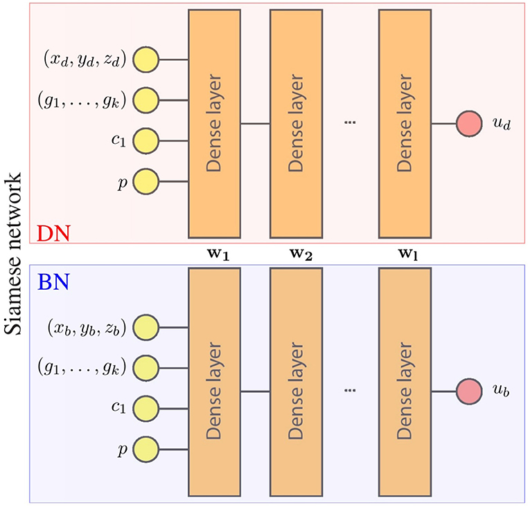
Figure 1. Surrogate network architecture for one component of the displacement field. w_i represents parameters of the i-th layer that are the shared by the boundary network (BN) and the domain network (DN). During training, both networks optimize these shared parameters with different data, leading to a single network with parameters {w₁, …, w_l} that meet the conditions of both networks (boundary and domain constrains).

We choose a loss functions that combines the L₂-norm error of BN and DN networks by means of a mixture parameter as follows

$\begin{array}{ll}l({B})={\displaystyle \sum _{{\text{u}}_d\in {{B}}_d}}\parallel {\text{u}}_d-{\tilde{\text{u}}}_d{\parallel }_{L_2}+\alpha {\displaystyle \sum _{{\text{u}}_b\in {{B}}_b}}\parallel {\text{u}}_b-{\tilde{\text{u}}}_b{\parallel }_{L_2}& (11)\end{array}$

where ${{B}}_b$ and ${{B}}_d$ are sets of points (training batches) on the boundary and inside the domain, respectively, u_i and ${\tilde{\text{u}}}_i$ are the displacements predicted with the neural network and the FE model, respectively, α is the penalty for the Dirichlet boundary conditions, and ${B}={{B}}_b+{{B}}_d$ is a given training batch. During training, two batches of the same size are fed in parallel to BN and DN, one with points over the boundary and one with points inside the domain. Then, the loss values from BN and DN are added and a back-propagation process updates the network weights.

2.4. Intrinsic Learning Domain

Training networks over a domain that is sparse (see Figure 3, Ω_PCA is only defined sparsely through x, y, z in the Cartessian coordinates) can be challenging due to the large degree of uncertainty in the non-sampled (or non-defined) regions. Moreover, as the coordinates are defined in a global Cartesian reference frame, the kinematic description can be too complex and higher-order approximants (or higher-capacity networks) would be required to approximate it. In turn, higher-order approximants will require larger datasets to properly define the unknown parameters through optimization.

To tackle such issues, we ideally want a reference domain in which the solution field is continuous, can be described by lower-order approximants, and where the dataset samples are evenly and contiguously spaced. To obtain that space, while preserving the topology of the geometry, we morph the reference domain to an intrinsic learning domain by means of a diffeomorphic mapping.

In this case, we map the reference domain Ω_PCA into a cylindrical representation of the LV Ω_learn (see Figure 2). The mapping is performed by stretching the ventricle base to be the outer radius of a cylinder, and fixing the central axis of the cylinder to be the apex of the heart. In this description, the axial direction is the intramural direction. Figure 2 shows the relationship between image, reference, and learning domains and their mappings. Note that by constructing these mapping functions, we can obtain the description of the fields in any domain.

FIGURE 2

Figure 2. Morphing procedure between reference Ω_PCA and learning Ω_learn. The top and bottom surface of the Ω_learn correspond to the endocardial surface and epicardial surface of the myocardium, respectively. The outer-radial surface corresponds to the base of the heart (beige surface). The gold spheres represent material points sampled from the geometry to help visualize the morphing process.

FIGURE 3

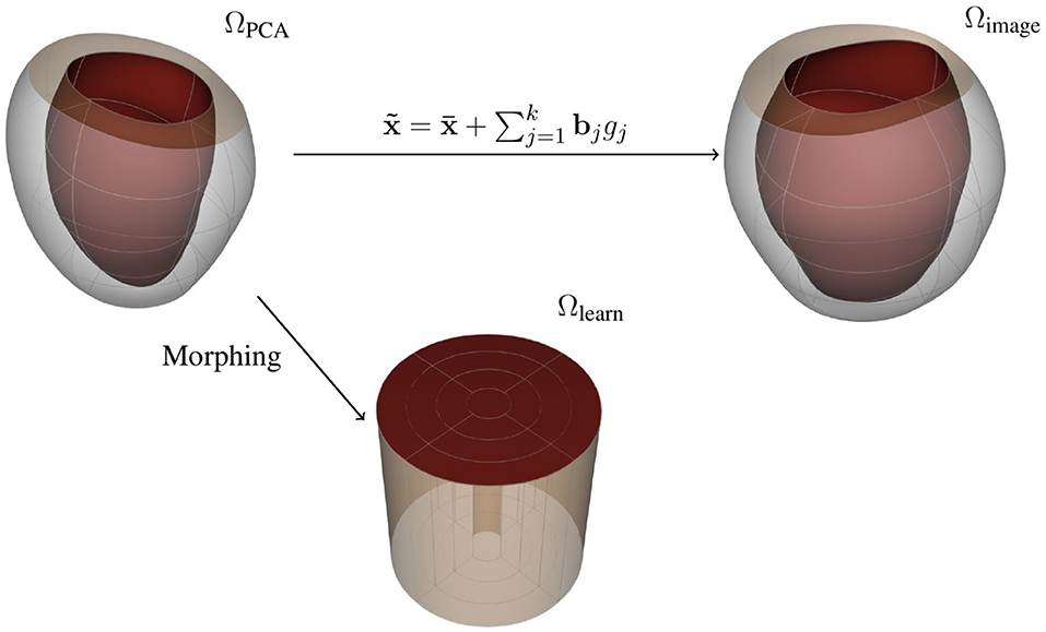
Figure 3. Representations for the free-load LV: (top left) reference domain, (top right) image domain, and (bottom) learning domain.

3. Results

3.1. Training Data

To construct the LV representation, we performed PCA over reconstructions of 28 in-vivo MRI sequences discretized by 1200 FE nodal points. We performed a statistical shape analysis on these reconstructions, as detailed in section 2.2. We assessed the accuracy of the PCA approximation space by means of the cumulative variance ${\widehat{\sigma }}_k^2$ introduced in Equation (10) to determine the necessary number of components to generate an acceptable representation of the LV. Figure 4 illustrates the improvement of the representation as more principal components are included into the space. We selected to use the approximation space of 2 principal components, accounting for 78.51% of the variability observed across the geometries. A qualitative interpretation of these two selected components is depicted in Figure 5, where g₁ has an important scaling contribution while g₂ increases the axial curvature and basal tilt of the chamber.

FIGURE 4

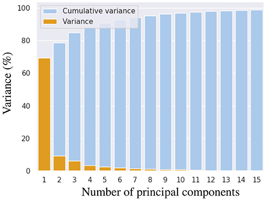
Figure 4. Cumulative variance in shape that is explained when increasing number of principal components are used for representing left ventricular geometry.

FIGURE 5

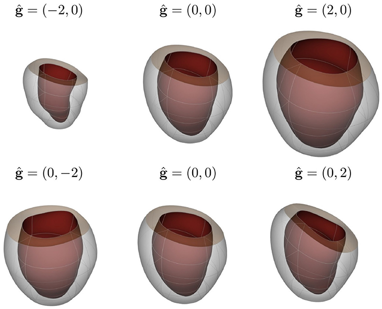
Figure 5. Visualization of LV shape related to the first two principal components of shape variation seen across the population of individuals considered in this study (first and second rows correspond to g₁ and g₂, respectively). The mean shape is shown in the central column, while the weights corresponding to −2 and 2 standard deviations (ĝ_j = ±2, j = 1, 2) are shown together with the mean shape for each principal component in the left and right columns, respectively.

To construct our training and testing datasets, we sampled geometries over the PCA-space and then predicted the displacement field for different loading conditions and material properties by means of our FE model. In this analysis, we considered a reduced PCA space with k = 2 principal components for reconstructing approximate LV geometries using Equation (8). Therefore, only weights w = {w₁, w₂} were specified to generate an LV geometry. We extracted equidistant samples of these weights using a step of Δs = 0.5 within the range [−2, 2] over each component of w, leading to 81 geometries. For each of those geometries, we performed FEM predictions for 10 different endocardial surface pressure loading conditions (generated from an in vivo trace with 10 time-points) with 7 different samples of the c₁ material parameter in the Guccione constitutive relation ($c_1^i=2+i0.5,i=0,1,\dots ,6$ within physiological ranges). Typical mammalian values were used for the remaining parameters of the Guccione relation (where c₂ = 8.61, c₃ = 3.67, c₄ = 25.77) to ensure physiologically plausible anisotropic mechanical responses for the myocardium [25]. This yielded 70 mechanical problems per geometry. Additionally, each geometry was sampled at 1108 domain points, which were equally spaced inside each mesh element. Thus, a total of ~ 6M samples were obtained from the FE models (see Table 1).

TABLE 1

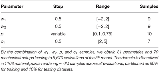
Table 1. Sampling of the geometrical and mechanical parameters used to generate training and testing dataset.

We partitioned the samples as 90% for training and 10% for testing datasets, using the former dataset to train DN. To impose an homogeneous Dirichlet boundary condition at BN, we dynamically generated batches of random points along the boundary, prescribing $\tilde{d}=0$ in the BN loss function. These dynamically generated points yielded better results than assimilation of the values at the mesh boundary nodes.

The networks were trained using the ADAM algorithm [26] with the parameters α = 0.01, β₁ = 0.9, and β₂ = 0.999 and a batch size of 5, 000 samples during 500 epochs. During testing, we computed the loss function among all cases in the testing dataset to assess the performance of the network. After finishing all training epochs, we assigned the network weights as those associated with the lowest loss value among all testing epochs.

3.2. Evaluation Metrics

The error of the network prediction was assessed in terms of absolute and relative L₂-norm errors. For a single case—i.e., a mechanical problem with a single set of boundary, material, and loading conditions—, the errors in the displacements over the entire mesh are computed as follows

$\begin{array}{ll}{\epsilon }_{\text{abs}}=\parallel {\text{u}}_{\text{FEM}}-{\text{u}}_{\text{DL}}{\parallel }_{L_2}& (12)\end{array}$

$\begin{array}{ll}{\epsilon }_{\text{rel}}=\frac{\parallel {\text{u}}_{\text{FEM}}-{\text{u}}_{\text{DL}}{\parallel }_{L_2}}{\parallel {\text{u}}_{\text{FEM}}{\parallel }_{L_2}}& (13)\end{array}$

where u_FEM are the ground truth displacements from the FE model and u_DL are the displacements predicted by the network. The adimensionalized quantity ε_rel allows a statistical comparison of errors among different loading conditions without biasing toward contributions from the cases with larger displacements.

3.3. Training in Reference and Learning Domains

The surrogate network was trained in the reference and learning domains using the same dataset (described in section 3.1) to compare the performance of our method when different representation spaces were employed during training. The sensitivity of the method's accuracy with respect to the network architecture was also analyzed for different numbers of layers and neurons. This involved training networks with 2, 3, and 4 identical layers, each of which consisted of three different cases with 32, 64, and 128 neurons per layer, yielding a total of nine different architectures. The accuracy was quantified in terms of the relative error ε_rel. This allowed us to quantify the overall error ratio in predicting the displacement field.

The relative error was computed through all cases in the testing dataset (mean and standard deviation of ε_rel are reported in Table 2). The mean relative error across all architectures was 10.78 times lower when using the learning domain compared with the reference domain, showing a clear improvement in the learning capabilities by modifying the training domain. Of particular note, the best-ranked model (the one with the lowest μ_εrel) presented an error of 4.4 ± 2.9%. Interestingly, the relative error has higher sensitivity when displacements are smaller, i.e., lower pressures and larger elasticity values (see Figure 6). In terms of absolute displacement error, the μ_εabs is directly proportional to the displacement, but not through a linear relationship as indicated by ε_rel. Hence, the surrogate model favors cases with larger displacements in terms of accuracy. Note that such behavior is a consequence of the selected loss function (11), which penalizes the absolute displacement error during training.

TABLE 2

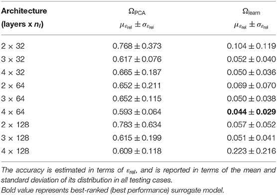
Table 2. Prediction error for the surrogate model trained in the reference domain Ω_PCA and learning domain Ω_learn.

FIGURE 6

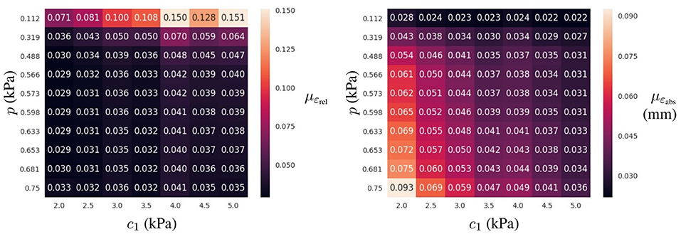
Figure 6. Prediction error for the best-ranked surrogate model (4 layers of 64 neurons trained in Ω_learn) for the testing dataset: mean ε value (Left) and mean absolute displacement error (Right) for a given loading condition (p in the vertical axis) and material property (c₁ in the horizontal axis) across all geometries in the testing dataset.

3.4. Analysis of the Surrogate Model Error

To further characterize the surrogate model error, we analyzed influences of the geometry, pressure loading, and material properties on the error distribution. In the previous section, we found that the relative errors were higher for mechanical problems with the smaller loads or the stiffer material properties. To understand the distribution of such errors across the PCA-space, we computed ε_rel for the 81 geometries described in section 3.1 and analyzed its distribution for three different materials (with c₁ values for a softer, an intermediate and a stiffer model of myocardium) under the range of physiological pressures during the filling of the LV chamber (see Figure 7). We observed that lower pressures not only increased the mean relative error, but also resulted in a wider spread in its distribution (higher ε_rel values were associated with higher g₁ values), indicating that some parts of the PCA-space are more affected by the error than others. A similar effect was observed when increasing the stiffness of the LV. Increasing c₁ led to a wider error distribution with a larger effect in the low pressure regime (as can be observed by comparing relative stretching of the violins for p < 0.4 vs. p > 0.4).

FIGURE 7

Figure 7. Distribution of ε_rel for the best-ranked surrogate model across all 81 geometries generated (training and testing datasets combined) leading to 81 samples per violin. From left to right, the error is presented for three different material properties c₁ = 2, 3.5, and 5 kPa, and each model was loaded with 10 different pressures.

Regarding the spatial distribution of the error, no specific pattern was found, although the errors tend to localize toward the base of the LV (see Figures 8, 9). As mentioned previously, an increase in pressure and decrease in stiffness results in an increment of ε_abs but does not change its spatial distribution. Conversely, geometrical variations result in changes in error distribution as expected (see Figure 9). Furthermore, an increment of error and overall displacements is observed as ĝ₁ increases which is related to the fact that this principal component scales with the LV size.

FIGURE 8

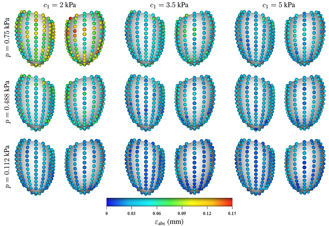
Figure 8. Mean intramural spatial distribution of ε_abs for a fixed set of geometrical parameters ĝ₁ = 0 and ĝ₂ = 0 in the anterior and posterior views of the LV: (horizontal axis) variations in the material properties (c₁ = 2, 3.5, and 5 kPa); and (vertical axis) variations in the loading conditions (p = 0.112, 0.488, and 0.75 kPa). For each pair of images, the posterior surface of the heart is shown on the left and the anterior surface is shown on the right.

FIGURE 9

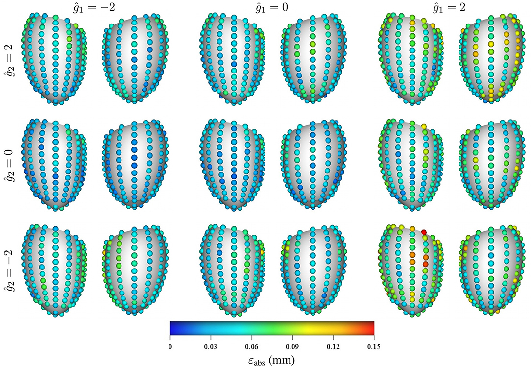
Figure 9. Mean intramural spatial distribution of ε_abs for a fixed set of mechanical properties p = 0.488 kPa and c₁ = 3.5 kPa: (left to right) variations in the geometric parameter ĝ₁ = −2, 0, and 2; and (bottom to top) variations in the geometric parameter ĝ₂ = −2, 0, and 2. For each pair of images, the posterior surface of the heart is shown on the left and the anterior surface is shown on the right.

3.5. Performance Assessment

To highlight the increase in performance, we recorded the wall clock time for the FEM and surrogate models to simulate the LV filling process at 10 different time points. Each simulation (of 10 time points) was repeated 10 times to evaluate the mean performance and its standard deviation. The FEM model was implementation in OpenCMISS (refer to section 2.1 and references within for further details) and executed in an Intel Xeon Gold 6136 CPU at 3.00GHz for a duration of 44.515 ± 0.484 seconds per simulation. The surrogate model was implemented in TensorFlow v1.12 and executed in a TitanXP GPU with a duration of 0.704 ± 0.056 seconds per simulation. The proposed model presented a mean acceleration of 62.23 times with respect to a traditional FEM simulation.

4. Discussion

This work presents a surrogate model capable of reproducing FEM predictions of a load-free LV mechanical model 62.23 times faster with an overall error of 4.4%. Deeper networks would render even more accurate results but would result in longer training times, more memory consumption and larger computational times for predictions. This particular trade-off should be studied for each specific application and its clinical demands. The error in the surrogate model is the difference between the surrogate model predictions and the trainer model predictions (in this case, the FE model predictions) and is expected to be trainer-model-dependent. If a more complex training model is used, the surrogate network may require a deeper and wider architecture to maintain the same order of accuracy. Also, the methodology deals with geometric variations of the domain by encoding them in a finite set of parameters by means of principal component analysis. A similar approach has been adopted in Liang et al. [18] for the assessment of wall shear stress in the aorta. Our strategy presents an important step toward translation of computational models to clinical practice. In this particular case, our surrogate model assimilated the mechanical behavior from a FEM model although the methodology is independent of the computational strategy (e.g., FEM, finite volume method, mesh-free methods, or finite difference approximations). The strategy is interestingly appealing in scenarios where large number of simulations are required, such as inverse problems for mechanical or geometrical parameter identification, or applications that require fast response times such as real-time simulations for risk assessment during therapeutic treatments or for teaching purposes.

The intrinsic learning domain introduced in this work produced a significant increase in the surrogate model performance, gaining one order of magnitude in accuracy with respect to using the Cartesian description of the LV. Traditional approaches for improving the surrogate model accuracy would have required increasing the size of the dataset that would result in a larger training process and refinements to the FEM model to compute such new data (which in some cases can lead to intractable computational cost). This issue is even more prohibitive for complex multi-physics models where only small datasets can be generated in a reasonable execution time. The proposed domain relaxes such requirements, easing the data generation and training process, and is therefore more beneficial for training HPC and multi-physics models than using traditional Cartesian description. Generalizing this methodology to other mechanics problems, or more complex domains such as bi-ventricular or whole-heart models, could be achieved by automating the morphing task for obtaining the intrinsic learning domain. Flattening-based strategies [27] may provide such a solution for 2D domains meanwhile 3D domains may exploit the 2D solution to project its surfaces and map the internal points by means of an optimization problem. Overall, we showed that the choice of the representation domain upon which the training is performed, is of utmost importance for the performance and training of the network.

Here, we addressed the estimation of three scalar fields by predicting each field in a decoupled manner by means of a different neural network. This approach can be extended straightforwardly to compute as many fields as needed. Nevertheless, multi-physics problems can benefit through the use of networks that predict more than one field at the time, allowing the network to learn the correlation among the fields. In our particular problem, the prediction of the three fields by a single neural network yielded lower accuracy than its decoupled counterpart.

The FEM model, employed in this work, was a simple phenomenological model that approximates the left ventricle inflation phenomenon. Contractile, multi-scale or multi-physics cardiac models present more complex behavior involving higher-order and non-linear responses. This will impact the network architecture required to approximate the physical fields of interest, where deeper and wider layers of neurons in the surrogate model may be better suited to reproduce such models. It is noteworthy that only the target physical field to be learnt would change, thus the presented methodology and learning space is still valid for such cases.

Another interesting aspect is the independence from the dataset generator. We chose to employ a computational model because of the availability and control over the model. However, a similar study could be conducted using experimental data, as long as all relevant mechanical parameters are identifiable, turning the surrogate model into a mechanical model per se. An advantage of this approach is that it provides the capabilities of neural networks to model non-linear contributions by construction (most activation functions are non-linear) and offers a universal approximator for continuous functions [28] in contrast to traditional computational models.

While great strides have been made for modeling LV mechanics, a number of issues remain before reliable and accurate LV models can be incorporated in medical practice. During construction of the PCA spaces, it is difficult to establish point-to-point correspondence between reconstructions of different subjects due to the difficulty to find multiple anatomical landmarks throughout the myocardium. Also, the lack of myocardial texture in the MR images hinders the estimation of displacements inside the muscle, encumbering the definition of appropriate boundary conditions for the displacement at the base of the LV. Also, a non-invasive and reliable methodology to determine the inner ventricular pressure would be beneficial to determine the stiffness of the LV by means of this model in a clinical setup.

5. Conclusions

In this work, we presented a surrogate model of the load-free left ventricle that was capable of predicting the heart's displacement field during passive inflation under physiological loading conditions and material properties. To the best of our knowledge, our model is the first to account for physiologically realistic geometric variations of the myocardium for training machine learning based mechanical models. Additionally, we introduce a novel representation domain to increase the accuracy of the model and ease the training task. The surrogate model trained with 28 in vivo geometries produced an error of just 4.4% compared with FEM simulations while increasing its performance by more than 62 times, delivering simulations in 0.7 s. The analysis of the model error showed a higher relative accuracy for larger displacements given by larger loading conditions or less stiffer material properties. The model developed in this study is suitable for a number of applications including the characterization of the myocardial material properties and quantifying uncertainties associated with cardiac mechanics modeling.

Data Availability Statement

The datasets generated for this study are available on request to the corresponding author.

Author Contributions

GM designed the study, implemented, trained, and validated the machine learning networks, and prepared the manuscript. TB developed the biomechanical modeling framework, performed the PCA, and contributed to the design of the study and the manuscript text. MS contributed to the design of the study. MN contributed to the design of the study, the development of the biomechanical modeling framework, and edited the manuscript.

Funding

GM was funded by the Li Ka Shing Foundation. This work was supported by research funding grants 13/317 and 17/608 from the Health Research Council of New Zealand.

Conflict of Interest

GM was supported by research funding grant 9077/31/8402 from the Li Ka Shing Foundation and received an NVIDIA GPU Grant from NVIDIA Corporation. This work was supported by research funding grants 13/317 and 17/608 from the Health Research Council of New Zealand. The NVIDIA Corporation was not involved in the study design, collection, analysis, interpretation of data, the writing of this article or the decision to submit it for publication.

The remaining authors declare that the research was conducted in the absence of any commercial or financial relationships that could be construed as a potential conflict of interest.

Acknowledgments

We gratefully acknowledge the support of NVIDIA Corporation with the donation of the Titan Xp GPU used for this research.

References

1. Niederer SA, Lumens J, Trayanova NA. Computational models in cardiology. Nat Rev Cardiol. (2019) 16:100–11. doi: 10.1038/s41569-018-0104-y

PubMed Abstract | CrossRef Full Text | Google Scholar

2. Niederer SA, Smith NP. Using physiologically based models for clinical translation: predictive modelling, data interpretation or something in-between? J Physiol. (2016) 594:6849–63. doi: 10.1113/JP272003

PubMed Abstract | CrossRef Full Text | Google Scholar

3. Wang ZJ, Wang VY, Bradley CP, Nash MP, Young AA, Cao JJ. Left ventricular diastolic myocardial stiffness and end-diastolic myofibre stress in human heart failure using personalised biomechanical analysis. J Cardiovasc Transl Res. (2018) 11:346–56. doi: 10.1007/s12265-018-9816-y

PubMed Abstract | CrossRef Full Text | Google Scholar

4. Wang VY, Nielsen PMF, Nash MP. Image-based predictive modeling of heart mechanics. Annu Rev Biomed Eng. (2015) 17:351–83. doi: 10.1146/annurev-bioeng-071114-040609

PubMed Abstract | CrossRef Full Text | Google Scholar

5. Chabiniok R, Wang VY, Hadjicharalambous M, Asner L, Lee J, Sermesant M, et al. Multiphysics and multiscale modelling, data–model fusion and integration of organ physiology in the clinic: ventricular cardiac mechanics. Interface Focus. (2016) 6:20150083. doi: 10.1098/rsfs.2015.0083

PubMed Abstract | CrossRef Full Text | Google Scholar

6. Morris PD, Narracott A, Tengg-Kobligk Hv, Soto DAS, Hsiao S, Lungu A, et al. Computational fluid dynamics modelling in cardiovascular medicine. Heart. (2016) 102:18–28. doi: 10.1136/heartjnl-2015-308044

PubMed Abstract | CrossRef Full Text | Google Scholar

7. Oberkampf WL, Roy CJ. Verification and Validation in Scientific Computing. Cambridge, UK: Cambridge University Press (2010).

Google Scholar

8. Pathmanathan P, Cordeiro JM, Gray RA. Comprehensive uncertainty quantification and sensitivity analysis for cardiac action potential models. Front Physiol. (2019) 10:721. doi: 10.3389/fphys.2019.00721

PubMed Abstract | CrossRef Full Text | Google Scholar

9. Sirignano J, Spiliopoulos K. DGM: A deep learning algorithm for solving partial differential equations. J Comput Phys. (2018) 375:1339–64. doi: 10.1016/j.jcp.2018.08.029

CrossRef Full Text | Google Scholar

10. Rudd K, Ferrari S. A constrained integration (CINT) approach to solving partial differential equations using artificial neural networks. Neurocomputing (2015) 155:277–85. doi: 10.1016/j.neucom.2014.11.058

CrossRef Full Text | Google Scholar

11. Lagaris IE, Likas A, Fotiadis DI. Artificial neural networks for solving ordinary and partial differential equations. IEEE Trans Neural Netw. (1998) 9:987–1000. doi: 10.1109/72.712178

PubMed Abstract | CrossRef Full Text | Google Scholar

12. Lagaris IE, Likas AC, Papageorgiou DG. Neural-network methods for boundary value problems with irregular boundaries. IEEE Trans Neural Netw. (2000) 11:1041–9. doi: 10.1109/72.870037

PubMed Abstract | CrossRef Full Text | Google Scholar

13. McFall KS, Mahan JR. Artificial neural network method for solution of boundary value problems with exact satisfaction of arbitrary boundary conditions. IEEE Trans Neural Netw. (2009) 20:1221–33. doi: 10.1109/TNN.2009.2020735

PubMed Abstract | CrossRef Full Text | Google Scholar

14. Berg J, Nyström K. A unified deep artificial neural network approach to partial differential equations in complex geometries. Neurocomputing (2018) 317:28–41. doi: 10.1016/j.neucom.2018.06.056

CrossRef Full Text | Google Scholar

15. Raissi M, Perdikaris P, Karniadakis GE. Physics-informed neural networks: a deep learning framework for solving forward and inverse problems involving nonlinear partial differential equations. J Comput Phys. (2019) 378:686–707. doi: 10.1016/j.jcp.2018.10.045

CrossRef Full Text | Google Scholar

16. Raissi M, Perdikaris P, Karniadakis GE. Machine learning of linear differential equations using Gaussian processes. J Comput Phys. (2017) 348:683–93. doi: 10.1016/j.jcp.2017.07.050

CrossRef Full Text | Google Scholar

17. Raissi M. Deep hidden physics models: deep learning of nonlinear partial differential equations. J Mach Learn Res. (2018) 19:932–55. Available online at: http://jmlr.org/papers/v19/18-046.html

Google Scholar

18. Liang L, Liu M, Martin C, Sun W. A deep learning approach to estimate stress distribution: a fast and accurate surrogate of finite-element analysis. J R Soc Interface. (2018) 15:20170844. doi: 10.1098/rsif.2017.0844

PubMed Abstract | CrossRef Full Text | Google Scholar

19. Swischuk R, Mainini L, Peherstorfer B, Willcox K. Projection-based model reduction: formulations for physics-based machine learning. Comput Fluids. (2019) 179:704–17. doi: 10.1016/j.compfluid.2018.07.021

CrossRef Full Text | Google Scholar

20. Nielsen PM, Le Grice IJ, Smaill BH, Hunter PJ. Mathematical model of geometry and fibrous structure of the heart. Am J Physiol Heart Circul Physiol. (1991) 260:H1365–78. doi: 10.1152/ajpheart.1991.260.4.H1365

PubMed Abstract | CrossRef Full Text | Google Scholar

21. Guccione JM, McCulloch AD, Waldman LK. Passive material properties of intact ventricular myocardium determined from a cylindrical model. J Biomech Eng. (1991) 113:42–55. doi: 10.1115/1.2894084

PubMed Abstract | CrossRef Full Text | Google Scholar

22. Nash MP, Hunter PJ. Computational mechanics of the heart. J Elast Phys Sci Solids. (2000) 61:113–41. doi: 10.1007/0-306-48389-0_4

CrossRef Full Text | Google Scholar

23. Bradley C, Bowery A, Britten R, Budelmann V, Camara O, Christie R, et al. OpenCMISS: a multi-physics & multi-scale computational infrastructure for the VPH/Physiome project. Prog Biophys Mol Biol. (2011) 107:32–47. doi: 10.1016/j.pbiomolbio.2011.06.015

PubMed Abstract | CrossRef Full Text | Google Scholar

24. Golub GH, Reinsch C. Singular value decomposition and least squares solutions. Numer Math. (1970) 14:403–20. doi: 10.1007/BF02163027

CrossRef Full Text | Google Scholar

25. Wang VY, Lam HI, Ennis DB, Cowan BR, Young AA, Nash MP. Modelling passive diastolic mechanics with quantitative MRI of cardiac structure and function. Med Image Anal. (2009) 13:773–84. doi: 10.1016/j.media.2009.07.006

PubMed Abstract | CrossRef Full Text | Google Scholar

26. Kingma DP, Ba J. Adam: a method for stochastic optimization. arXiv preprint arXiv:14126980 (2014). Available online at: https://arxiv.org/pdf/1412.6980

Google Scholar

27. Kreiser J, Meuschke M, Mistelbauer G, Preim B, Ropinski TA. Survey of flatteningbased medical visualization techniques. Graph Forum. (2018) 37:597–624.

Google Scholar

28. Lu Z, Pu H, Wang F, Hu Z, Wang L. The expressive power of neural networks: a view from the width. In: Advances in Neural Information Processing Systems. Long Beach, CA (2017). p. 6231–9.

Google Scholar