Large Time Behavior on the Linear Self-Interacting Diffusion Driven by Sub-Fractional Brownian Motion With Hurst Index Large Than 0.5 I: Self-Repelling Case

Let S^H be a sub-fractional Brownian motion with index $\frac{1}{2}<H<1$. In this paper, we consider the linear self-interacting diffusion driven by S^H, which is the solution to the equation

$d{X}_t^H=d{S}_t^H-\theta \left({\int }_0^t\left(X_t^H-X_s^H\right)ds\right)dt+\nu dt,X_0^H=0,$

where θ < 0 and $\nu \in \mathbb{R}$ are two parameters. Such process X^H is called self-repelling and it is an analogue of the linear self-attracting diffusion [Cranston and Le Jan, Math. Ann. 303 (1995), 87–93]. Our main aim is to study the large time behaviors. We show the solution X^H diverges to infinity, as t tends to infinity, and obtain the speed at which the process X^H diverges to infinity as t tends to infinity.

1 Introduction

In 1995, Cranston and Le Jan [1] introduced a linear self-attracting diffusion

$X_t=B_t-\theta {\int }_0^t{\int }_0^s\left(X_s-X_u\right)duds+\nu t,t\ge 0$(1.1)

with θ > 0 and X₀ = 0, where B is a 1-dimensional standard Brownian motion. They showed that the process X_t converges in L² and almost surely, as t tends infinity. This is a special case of path dependent stochastic differential equations. Such path dependent stochastic differential equation was first developed by Durrett and Rogers [2] introduced in 1992 as a model for the shape of a growing polymer (Brownian polymer) as follows

$X_t=X_0+B_t+{\int }_0^t{\int }_0^{s}f\left(X_s-X_u\right)duds,$(1.2)

where B is a d-dimensional standard Brownian motion and f is Lipschitz continuous. X_t corresponds to the location of the end of the polymer at time t. Under some conditions, they established asymptotic behavior of the solution of stochastic differential equation and gave some conjectures and questions. The model is a continuous analogue of the notion of edge (resp. vertex) self-interacting random walk. If f(x) = g(x)x/‖x‖ and g(x) ≥ 0, X_t is a continuous analogue of a process introduced by Diaconis and studied by Pemantle [3]. Let ${\mathcal{L}}^X(t,x)$ be the local time of the solution process X. Then, we have

$X_t=X_0+B_t+{\int }_0^{t}ds{\int }_{\mathbb{R}}f\left(-x\right){\mathcal{L}}^X\left(s,X_s+x\right)dx$

for all t ≥ 0. This formulation makes it clear how the process X interacts with its own occupation density. We may call this solution a Brownian motion interacting with its own passed trajectory, i.e., a self-interacting motion. In general, the Eq. 1.2 defines a self-interacting diffusion without any assumption on f. If

$x\cdot f\left(x\right)\ge 0\left(x\cdot f\left(x\right)\le 0\right)$

for all $x\in {\mathbb{R}}^d$, we call it self-repelling (resp. self-attracting). In 2002, Benaïm et al [4] also introduced a self-interacting diffusion with dependence on the (convolved) empirical measure. A great difference between these diffusions and Brownian polymers is that the drift term is divided by t. It is noteworthy that the interaction potential is attractive enough to compare the diffusion (a bit modified) to an Ornstein-Uhlenbeck process, in many case of f, which points out an access to its asymptotic behavior. More works can be found in Benaïm et al. [5], Cranston and Mountford [6], Gauthier [7], Herrmann and Roynette [8], Herrmann and Scheutzow [9], Mountford and Tarr [10], Shen et al [11], Sun and Yan [12] and the references therein.

On the other hand, starting from the application of fractional Brownian motion in polymer modeling, Yan et al [13] considered an analogue of the linear self-interacting diffusion:

$X_t^H=B_t^H-\theta {\int }_0^t{\int }_0^s\left(X_s^H-X_u^H\right)duds+\nu t,t\ge 0$(1.3)

with θ ≠ 0 and $X_0^H=0$, where B^H is a fractional Brownian motion (fBm, in short) with Hurst parameter $\frac{1}{2}\le H<1$. The solution of (1.3) is a Gaussian process. When θ > 0, Yan et al [13] showed that the solution X^H of (1.3) converges in L² and almost surely, to the random variable

$X_{\infty }^H={\int }_0^{\infty }{h}_{\theta }\left(s\right)d{B}_s^H+\nu {\int }_0^{\infty }{h}_{\theta }\left(s\right)ds$

where the function is defined ar follows

$h_{\theta }\left(s\right)=1-\theta s{e}^{\frac{1}{2}\theta s^2}{\int }_s^{\infty }{e}^{-\frac{1}{2}\theta u^2}du,s\ge 0$

with θ > 0. Recently, Sun and Yan [14] considered the related parameter estimations with θ > 0 and $\frac{1}{2}\le H<1$, and Gan and Yan [15] considered the parameter estimations with θ < 0 and $\frac{1}{2}\le H<1$.

Motivated by these results, as a natural extension one can consider the following stochastic differential equation:

$X_t=G_t-\theta {\int }_0^t{\int }_0^s\left(X_s-X_u\right)duds+\nu t,t\ge 0$(1.4)

with θ > 0 and X₀ = 0, where G = {G_t, t ≥ 0} is a Gaussian process with some suitable conditions which includes fractional Brownian motion and some related processes. However, for a (general) abstract Gaussian process it is difficult to find some interesting fine estimates associated with the calculations. So, in this paper we consider the linear self-attracting diffusion driven by a sub-fractional Brownian motion (sub-fBm, in short). We choose this kind of Gaussian process because it is only the generalization of Brownian motion rather than the generalization of fractional Brownian motion. It only has some similar properties of fractional Brownian motion, such as long memory and self similarity, but it has no stationary increment. The so-called sub-fBm with index H ∈ (0, 1) is a mean zero Gaussian process $S^H=\{S_t^H,t\ge 0\}$ with $S_0^H=0$ and the covariance

$R_H\left(t,s\right)\equiv E\left[S_t^H{S}_s^H\right]=s^{2H}+t^{2H}-\frac{1}{2}\left[{\left(s+t\right)}^{2H}+|t-s{|}^{2H}\right]$(1.5)

for all s, t ≥ 0. For H = 1/2, S^H coincides with the standard Brownian motion B. S^H is neither a semimartingale nor a Markov process unless H = 1/2, so many of the powerful techniques from stochastic analysis are not available when dealing with S^H. As a Gaussian process, it is possible to construct a stochastic calculus of variations with respect to S^H (see, for example, Alós et al [16]). The sub-fBm has properties analogous to those of fBm and satisfies the following estimates:

$\left[\left(2-2^{2H-1}\right)\wedge 1\right]{\left(t-s\right)}^{2H}\le E\left[{\left(S_t^H-S_s^H\right)}^2\right]\le \left[\left(2-2^{2H-1}\right)\vee 1\right]{\left(t-s\right)}^{2H}.$(1.6)

More works for sub-fBm and related processes can be found in Bojdecki et al. [17–20], Li [21–24], Shen and Yan [25, 26], Sun and Yan [27], Tudor [28–31], Ciprian A. Tudor [32] Yan et al [33–35] and the references therein.

In this present paper, we consider the linear self-interacting diffusion

$X_t^H=S_t^H-\theta {\int }_0^t{\int }_0^s\left(X_s^H-X_u^H\right)duds+\nu t,t\ge 0$(1.7)

with θ < 0 and $X_0^H=0$, where S^H is a sub-fBm with Hurst parameter $\frac{1}{2}\le H<1$. Our main aim is to show that the solution of (1.7) diverges to infinity and obtain the speed diverging to infinity, as t tends to infinity. The object of this paper is to expound and prove the following statements:

(I) For θ < 0 and $\frac{1}{2}<H<1$, the random variable

${\xi }_{\infty }^H={\int }_0^{\infty }s{e}^{\frac{1}{2}\theta s^2}d{S}_s^H$

exists as an element in L².

(II) For θ < 0 and $\frac{1}{2}<H<1$, as t → ∞, we have

$J_0^H\left(t;\theta ,\nu \right)≔t{e}^{\frac{1}{2}\theta t^2}{X}_t^H\to {\xi }_{\infty }^H-\frac{\nu }{\theta }$

in L² and almost surely.

(III) For θ < 0 and $\frac{1}{2}<H<1$, define the processes $J^H(n,\theta ,\nu )=\{J_t^H(n,\theta ,\nu ),t\ge 0\},n\ge 1$ by

$J_n^H\left(t;\theta ,\nu \right)≔\theta t^2\left(J_{n-1}^H\left(t;\theta ,\nu \right)-\left(2n-3\right)‼\left({\xi }_{\infty }^H-\frac{\nu }{\theta }\right)\right),n=\mathrm{1,2},\dots ,$

for all t ≥ 0, where (−1)!! = 1. We then have

$J_n^H\left(t;\theta ,\nu \right)\to \left(2n-1\right)‼\left({\xi }_{\infty }^H-\frac{\nu }{\theta }\right)$

holds in L² and almost surely for every n ≥ 1, as t → ∞.

This paper is organized as follows. In Section 2 we present some preliminaries for sub-fBm and Malliavin calculus. In Section 3, we obtain some lemmas. In Section 4, we prove the main result. In Section 5 we give some numerical results.

FIGURE 1

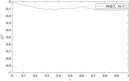
FIGURE 1. A path of X^H with θ = − 1 and H = 0.7.

FIGURE 2

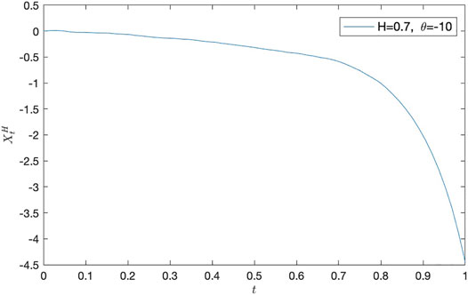
FIGURE 2. A path of X^H with θ = − 10 and H = 0.7.

FIGURE 3

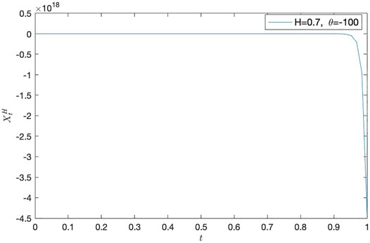
FIGURE 3. A path of X^H with θ = − 100 and H = 0.7.

FIGURE 4

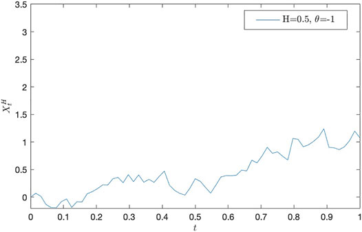
FIGURE 4. A path of X^H with θ = − 1 and H = 0.5.

FIGURE 5

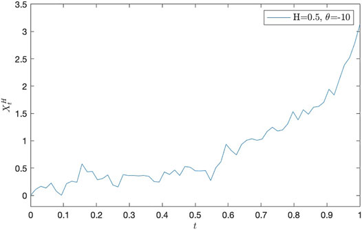
FIGURE 5. A path of X^H with θ = − 10 and H = 0.5.

FIGURE 6

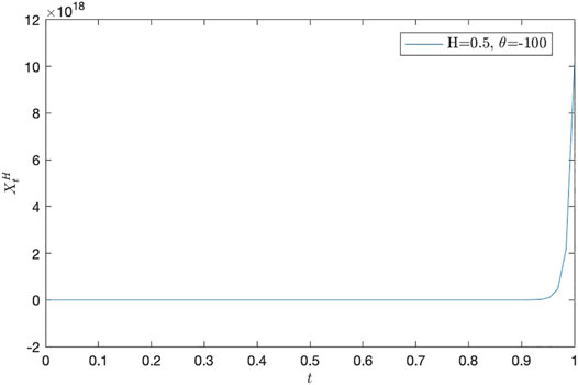
FIGURE 6. A path of X^H with θ = − 100 and H = 0.5.

TABLE 1

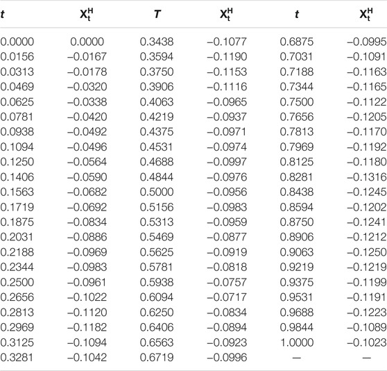
TABLE 1. The data of $X_t^H$ with θ = − 1 and H = 0.7.

TABLE 2

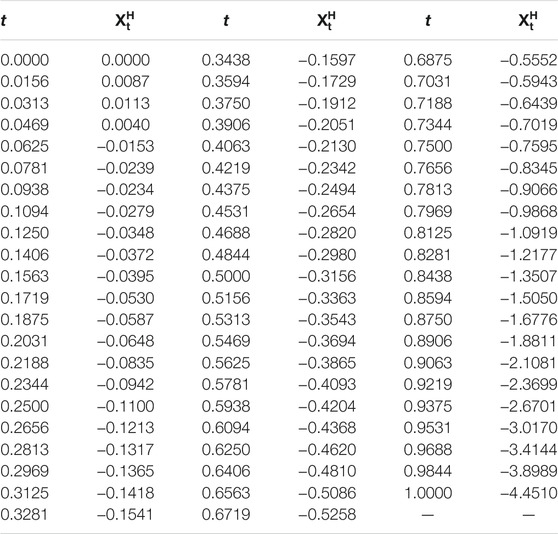
TABLE 2. The data of $X_t^H$ with θ = − 10 and H = 0.7.

TABLE 3

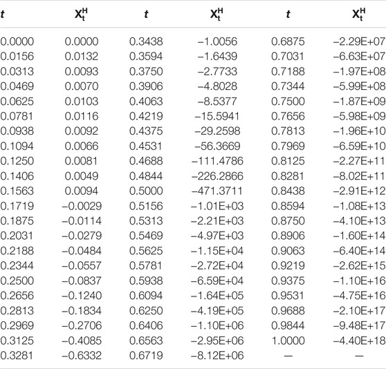
TABLE 3. The data of $X_t^H$ with θ = − 100 and H = 0.7.

TABLE 4

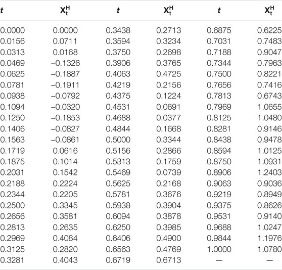
TABLE 4. The data of $X_t^H$ with θ = − 1 and H = 0.5.

TABLE 5

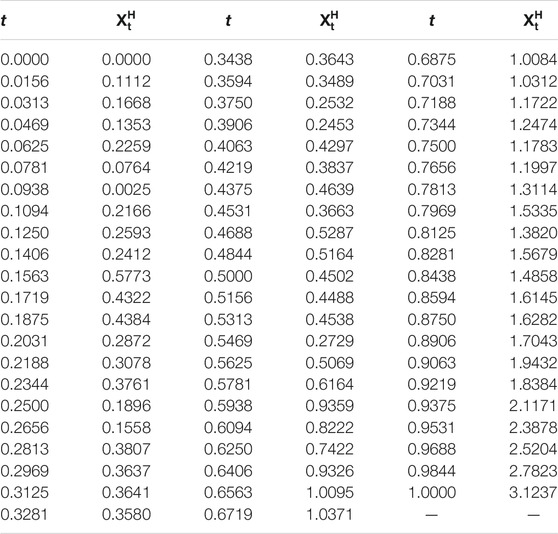
TABLE 5. The data of $X_t^H$ with θ = − 10 and H = 0.5.

TABLE 6

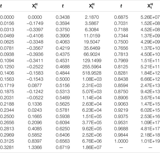
TABLE 6. The data of $X_t^H$ with θ = − 100 and H = 0.5.

2 Preliminaries

In this section, we briefly recall the definition and properties of stochastic integral with respect to sub-fBm. We refer to Alós et al [16], Nualart [36], and Tudor [31] for a complete description of stochastic calculus with respect to Gaussian processes. Throughout this paper we assume that $S^H=\left\{S_t^H,t\ge 0\right\}$ denotes a sub-fBm defined on the probability space $(\mathrm{\Omega },\mathcal{F},P)$ with index H. As we pointed out before, the sub-fBm S^H is a rather special class of self-similar Gaussian processes such that $S_0^H=0$, $E[S_t^H]=0$ and

$R^H\left(t,s\right)≔E\left[S_t^H{S}_s^H\right]=s^{2H}+t^{2H}-\frac{1}{2}\left[{\left(s+t\right)}^{2H}+|t-s{|}^{2H}\right]$(2.1)

for all s, t ≥ 0. For H = 1/2, S^H coincides with the standard Brownian motion B. S^H is neither a semimartingale nor a Markov process unless H = 1/2, so many of the powerful techniques from stochastic analysis are not available when dealing with S^H. As a Gaussian process, it is possible to construct a stochastic calculus of variations with respect to S^H. The sub-fBm appeared in Bojdecki et al [17] in a limit of occupation time fluctuations of a system of independent particles moving in ${\mathbb{R}}^d$ according a symmetric α-stable Lévy process, and it also appears in Bojdecki et al [18] in a high-density limit of occupation time fluctuations of the above mentioned particle system, where the initial Poisson configuration has finite intensity measure.

The estimate (1.6) and normality imply that the sub-fBm $t\mapsto S_t^H$ admits almost surely a bounded $\frac{1}{H-\vartheta }$-variation on any finite interval for any sufficiently small ϑ ∈ (0, H). That is, the paths of $t\mapsto S_t^H$ admits a bounded p_H-variation on any finite interval with $p_H>\frac{1}{H}$. As an immediate result, one can define the Young integral of a process u = {u_t, t ≥ 0} with respect to sub-fBm B^a,b

${\int }_0^t{u}_{s}d{S}_s^H$

as the limit in probability of a Riemann sum. Clearly, the integral is well-defined and

$u_t{S}_t^H={\int }_0^t{u}_{s}d{S}_s^H+{\int }_0^t{S}_s^{H}d{u}_s$

for all t ≥ 0, provided u is of bounded q_H-variation on any finite interval with q_H > 1 and $\frac{1}{p_H}+\frac{1}{q_H}>1$ (see, for examples, Bertoin [37] and FöIllmer [38]).

Let $\mathcal{H}$ be the completion of the linear space $\mathcal{E}$ generated by the indicator functions 1_[0,t], t ∈ [0, T] with respect to the inner product

${⟨1_{\left[0,s\right]},1_{\left[0,t\right]}⟩}_{\mathcal{H}}=R^H\left(t,s\right)$

for s, t ∈ [0, T]. When $\frac{1}{2}<H<1$, we can show that

$\begin{array}{ll}\hfill \Vert \phi {\Vert }_{\mathcal{H}}^2& ={\int }_0^T{\int }_0^T\phi \left(t\right)\phi \left(s\right)\frac{{\partial }^2}{\partial t\partial s}{R}^H\left(t,s\right)dsdt\hfill \\ \hfill & ={\int }_0^T{\int }_0^T\phi \left(t\right)\phi \left(s\right){\psi }_H\left(t,s\right)dsdt,\forall \phi \in \mathcal{H},\hfill \end{array}$

where

${\psi }_H\left(t,s\right)=\frac{{\partial }^2}{\partial t\partial s}{R}^{a,b}\left(t,s\right)=H\left(2H-1\right)\left(|t-s{|}^{2H-2}-|t+s{|}^{2H-2}\right)$

for s, t ∈ [0, T]. Define the linear mapping $\mathcal{E}\ni \phi \mapsto S^H(\phi )$ by

$1_{\left[0,t\right]}\mapsto S^H\left(1_{\left[0,t\right]}\right)={\int }_0^T{1}_{\left[0,t\right]}\left(s\right)d{S}_s^H\equiv S_t^H$

for all t ∈ [0, T] and it can be continuously extended to $\mathcal{H}$ and we call the mapping Φ is called the Wiener integral with respect to S^H, denoted by

$S^H\left(\phi \right)={\int }_0^T\phi \left(s\right)d{S}_s^H$

and

$\Vert \phi {\Vert }_{\mathcal{H}}^2=E{\left({\int }_0^T\phi \left(s\right)d{S}_s^H\right)}^2$(2.2)

for any $\phi \in \mathcal{H}$.

For simplicity, in this paper we assume that $\frac{1}{2}<H<1$. Thus, if for every T > 0, the integral

${\int }_0^T\phi \left(s\right)d{S}_s^H$

exists in L² and

${\int }_0^{\infty }{\int }_0^{\infty }\phi \left(t\right)\phi \left(s\right){\psi }_H\left(t,s\right)dsdt<\infty ,$

we can define the integral

${\int }_0^{\infty }\phi \left(s\right)d{S}_s^H$

and

$E{\left({\int }_0^{\infty }\phi \left(s\right)d{S}_s^H\right)}^2={\int }_0^{\infty }{\int }_0^{\infty }\phi \left(t\right)\phi \left(s\right){\psi }_H\left(t,s\right)dsdt.$

Denote by $\mathcal{S}$ the set of smooth functionals of the form

$F=f\left(S^H\left({\phi }_1\right),S^H\left({\phi }_2\right),\dots ,S^H\left({\phi }_n\right)\right),$

where $f\in C_b^{\infty }({\mathbb{R}}^n)$ and ${\phi }_i\in \mathcal{H}$. The Malliavin derivative D of a functional F as above is given by

$DF=\sum _{j=1}^n\frac{\partial f}{\partial x_j}\left(S^H\left({\phi }_1\right),S^H\left({\phi }_2\right),\dots ,S^H\left({\phi }_n\right)\right){\phi }_j.$

The derivative operator D is then a closable operator from L²(Ω) into $L^2(\mathrm{\Omega };\mathcal{H})$. We denote by ${\mathbb{D}}^{\mathrm{1,2}}$ the closure of $\mathcal{S}$ with respect to the norm

$\Vert F{\Vert }_{\mathrm{1,2}}≔\sqrt{E|F{|}^2+E\Vert DF{\Vert }_{\mathcal{H}}^2}.$

The divergence integral δ is the adjoint of derivative operator D^H. That is, we say that a random variable u in $L^2(\mathrm{\Omega };\mathcal{H})$ belongs to the domain of the divergence operator δ, denoted by Dom(δ^S), if

$E\left|{⟨DF,u⟩}_{\mathcal{H}}\right|\le c\Vert F{\Vert }_{L^2\left(\mathrm{\Omega }\right)}$

for every $F\in {\mathbb{D}}^{\mathrm{1,2}}$, where c is a constant depending only on u. In this case δ(u) is defined by the duality relationship

$E\left[F\delta \left(u\right)\right]=E{⟨DF,u⟩}_{\mathcal{H}}$(2.3)

for any $F\in {\mathbb{D}}^{\mathrm{1,2}}$. We have ${\mathbb{D}}^{\mathrm{1,2}}\subset \mathrm{D}\mathrm{o}\mathrm{m}(\delta )$ and for any $u\in {\mathbb{D}}^{\mathrm{1,2}}$

$\begin{array}{ll}\hfill E\left[\delta {\left(u\right)}^2\right]& =E\Vert u{\Vert }_{\mathcal{H}}^2+E{⟨Du,\left(Du\right)\ast ⟩}_{\mathcal{H}\otimes \mathcal{H}}\hfill \\ \hfill & =E\Vert u{\Vert }_{\mathcal{H}}^2+E{\int }_{{\left[0,T\right]}^4}{D}_{\xi }{u}_r{D}_{\eta }{u}_s{\varphi }_H\left(\eta ,r\right){\varphi }_H\left(\xi ,s\right)dsdrd\xi d\eta ,\hfill \end{array}$

where ${(D^{S}u)}^{\ast }$ is the adjoint of Du in the Hilbert space $\mathcal{H}\otimes \mathcal{H}$. We will denote

$\delta \left(u\right)={\int }_0^T{u}_s\delta S_s^H$

for an adapted process u, and it is called Skorohod integral. Alós et al [16], we can obtain the relationship between the Skorohod and Young integral as follows

${\int }_0^T{u}_{s}d{S}_s^H={\int }_0^T{u}_s\delta S_s^H+{\int }_0^T{\int }_0^T{D}_s{u}_t\psi \left(t,s\right)dsdt,$

provided u has a bounded q-variation with $1\le q<\frac{1}{H}$ and $u\in {\mathbb{D}}^{\mathrm{1,2}}(\mathcal{H})$ such that

${\int }_0^T{\int }_0^T{D}_s{u}_t\psi \left(t,s\right)dsdt<\infty .$

Theorem 2.1 (Alós et al [16]). Let 0 < H < 1 and let $f\in C^2(\mathbb{R})$ such that

$\max \left\{|f\left(x\right)|,|f^{\prime }\left(x\right)|,|f^{″}\left(x\right)|\right\}\le \kappa e^{\beta x^2},$(2.4)

where κ and β are two positive constants with $\beta <\frac{1}{4}{T}^{-2H}$. Then we have

$f\left(S_t^H\right)=f\left(0\right)+{\int }_0^t{f}^{\prime }\left(S_s^H\right)d{S}_s^H+H\left(2-2^{2H-1}\right){\int }_0^t{f}^{″}\left(S_s^H\right)s^{2H-1}ds$

for all t ∈ [0, T].

3 Some Basic Estimates

Throughout this paper we assume that θ < 0 and $\frac{1}{2}<H<1$. Recall that the linear self-interacting diffusion with sub-fBm S^H defined by the stochastic differential equation

$X_t^H=S_t^H-\theta {\int }_0^t{\int }_0^s\left(X_s^H-X_u^H\right)duds+\nu t,t\ge 0$(3.1)

with θ < 0. Define the kernel (t, s)↦h_θ(t, s) as follows

$h_{\theta }\left(t,s\right)=\left\{\begin{array}{cc}1-\theta s{e}^{\frac{1}{2}\theta s^2}{\int }_s^t{e}^{-\frac{1}{2}\theta u^2}du,\hfill & t\ge s,\hfill \\ 0,\hfill & t<s\hfill \end{array}\right.$(3.2)

for s, t ≥ 0. By the variation of constants method (see, Cranston and Le Jan [1]) or Itô’s formula we may introduce the following representation:

$X_t^H={\int }_0^t{h}_{\theta }\left(t,s\right)d{S}_s^H+\nu {\int }_0^t{h}_{\theta }\left(t,s\right)ds$(3.3)

for t ≥ 0.

The kernel function (t, s)↦h_θ(t, s) with θ < 0 admits the following properties (these properties are proved partly in Sun and Yan [12]):

• For all s ≥ 0, the limit

$\underset{t\to \infty }{\lim }\left(t{e}^{\frac{1}{2}\theta t^2}{h}_{\theta }\left(t,s\right)\right)=s{e}^{\frac{1}{2}\theta s^2}$(3.4)

for all s ≥ 0.

• For all t ≥ s ≥ 0, we have

$1\le h_{\theta }\left(t,s\right)\le e^{-\frac{1}{2}\theta \left(t^2-s^2\right)}.$

• For all t ≥ s, r ≥ 0, we have

$h_{\theta }\left(t,0\right)=h_{\theta }\left(t,t\right)=1,{\int }_s^t{h}_{\theta }\left(t,u\right)du=e^{\frac{1}{2}\theta s^2}{\int }_s^t{e}^{-\frac{1}{2}\theta u^2}du.$

Lemma 3.1 Let θ < 0 and define function

$I_{\theta }\left(t\right)=-\theta t{e}^{\frac{1}{2}\theta t^2}{\int }_0^t{e}^{-\frac{1}{2}\theta u^2}du-1.$

We then have $\underset{t\to \infty }{\lim }{t}^2{I}_{\theta }(t)=-\frac{1}{\theta }$ and

$\underset{t\to \infty }{\lim }{t}^2\left(1+\theta t{e}^{-\frac{1}{2}\theta t^2}{\int }_t^{\infty }{e}^{\frac{1}{2}\theta u^2}du\right)=-\frac{1}{\theta }$

Proof This is simple calculus exercise.

Lemma 3.2 (Sun and Yan [12]). Let θ < 0 and define the functions t↦I_θ(t, n), n = 1, 2, … as follows

$I_{\theta }\left(t,1\right)=-\theta t^2{I}_{\theta }\left(t\right),I_{\theta }\left(t,n+1\right)=-\theta t^2\left[I_{\theta }\left(t,n\right)-\left(2n-1\right)‼\right].$

Then we have

$\underset{t\to \infty }{\lim }{I}_{\theta }\left(t,n\right)=\left(2n-1\right)‼.$(3.5)

for every n ≥ 0, where (−1)! = 1.

Lemma 3.3 Let θ < 0. Then the integral

$\mathrm{\Delta }\left(H\right)={\int }_0^{\infty }{\int }_0^{\infty }xy{e}^{\frac{1}{2}\theta \left(x^2+y^2\right)}{\psi }_H\left(x,y\right)dxdy$(3.6)

converges and as t → ∞,

$\underset{t\to \infty }{\lim }{t}^2{e}^{-\theta t^2}E{\left(X_t^H\right)}^2=\mathrm{\Delta }\left(H\right).$

Proof An elementary may show that (3.6) converges for all θ < 0. It follows from L’Hôspital’s rule that

$\begin{array}{ll}\hfill \underset{t\to \infty }{\lim }& t^2{e}^{\theta t^2}E{\left(X_t^H\right)}^2=\underset{t\to \infty }{\lim }{t}^2{e}^{\theta t^2}{\int }_0^t{\int }_0^t{h}_{\theta }\left(t,x\right)h_{\theta }\left(t,y\right){\psi }_H\left(x,y\right)dxdy\hfill \\ \hfill & =\underset{t\to \infty }{\lim }\frac{{\theta }^2}{t^{-2}{e}^{-\theta t^2}}{\int }_0^{t}dx{\int }_0^{t}xy{e}^{\frac{1}{2}\theta \left(x^2+y^2\right)}{\psi }_H\left(x,y\right)dy{\int }_x^{t}du{\int }_y^t{e}^{-\frac{1}{2}\theta \left(u^2+v^2\right)}dv\hfill \\ \hfill & =2\underset{t\to \infty }{\lim }\frac{{\theta }^2}{t^{-2}{e}^{-\theta t^2}}{\int }_0^{t}du{\int }_0^{u}dx{\int }_0^{u}dv{\int }_0^{v}dyxy{e}^{\frac{1}{2}\theta \left(x^2+y^2-u^2-v^2\right)}{\psi }_H\left(x,y\right)\hfill \\ \hfill & =\underset{t\to \infty }{\lim }\frac{-\theta }{t^{-1}{e}^{-\frac{1}{2}\theta t^2}}{\int }_0^{t}dx{\int }_0^t{e}^{-\frac{1}{2}\theta v^2}dv{\int }_0^{v}xy{e}^{\frac{1}{2}\theta \left(x^2+y^2\right)}{\psi }_H\left(x,y\right)dy\hfill \\ \hfill & =\underset{t\to \infty }{\lim }\frac{-\theta }{t^{-1}{e}^{-\frac{1}{2}\theta t^2}}{\int }_0^t{e}^{-\frac{1}{2}\theta v^2}dv{\int }_0^{t}dx{\int }_0^{v}xy{e}^{\frac{1}{2}\theta \left(x^2+y^2\right)}{\psi }_H\left(x,y\right)dy\hfill \\ \hfill & =\underset{t\to \infty }{\lim }\frac{-\theta }{t^{-1}{e}^{-\frac{1}{2}\theta t^2}}{\int }_0^t{e}^{-\frac{1}{2}\theta v^2}dv{\int }_0^{v}dx{\int }_0^{v}xy{e}^{\frac{1}{2}\theta \left(x^2+y^2\right)}{\psi }_H\left(x,y\right)dy\hfill \\ \hfill & ={\int }_0^{\infty }dx{\int }_0^{\infty }xy{e}^{\frac{1}{2}\theta \left(x^2+y^2\right)}{\psi }_H\left(x,y\right)dy,\hfill \end{array}$

where we have used the following fact:

$\begin{array}{ll}\hfill \underset{t\to \infty }{\lim }& \frac{1}{t^{-1}{e}^{-\frac{1}{2}\theta t^2}}{\int }_0^t{e}^{-\frac{1}{2}\theta v^2}dv{\int }_v^{t}dx{\int }_0^{v}xy{e}^{\frac{1}{2}\theta \left(x^2+y^2\right)}{\psi }_H\left(x,y\right)dy\hfill \\ \hfill & =\underset{t\to \infty }{\lim }\frac{1}{t^{-1}{e}^{-\frac{1}{2}\theta t^2}}{\int }_0^{t}dx{\int }_0^x{e}^{-\frac{1}{2}\theta v^2}dv{\int }_0^{v}xy{e}^{\frac{1}{2}\theta \left(x^2+y^2\right)}{\psi }_H\left(x,y\right)dy=0.\hfill \end{array}$

This completes the proof.

Lemma 3.4 Let θ < 0. Then, convergence

$\underset{t\to \infty }{\lim }\frac{1}{t^{2-2H}}{e}^{-\theta t^2}{\int }_t^{\infty }{\int }_s^{\infty }sr{e}^{\frac{1}{2}\theta \left(s^2+r^2\right)}{\psi }_H\left(s,r\right)dsdr=\frac{1}{4}{\left(-\theta \right)}^{-2H}\mathrm{\Gamma }\left(2H+1\right).$(3.7)

holds.

Proof It follows from L’Hôspital’s rule that

$\begin{array}{ll}\hfill \underset{t\to \infty }{\lim }& \frac{1}{t^{2-2H}{e}^{\theta t^2}}{\int }_t^{\infty }u{e}^{\frac{1}{2}\theta u^2}\left({\int }_u^{\infty }v{e}^{\frac{1}{2}\theta v^2}{\psi }_H\left(u,v\right)dv\right)du\hfill \\ \hfill & =-\frac{1}{2\theta }\underset{t\to \infty }{\lim }\frac{1}{t^{2-2H}{e}^{\frac{1}{2}\theta t^2}}{\int }_t^{\infty }v{e}^{\frac{1}{2}\theta v^2}{\psi }_H\left(t,v\right)dv\hfill \\ \hfill & =-\underset{t\to \infty }{\lim }\frac{H\left(2H-1\right)}{2\theta t^{2-2H}}{\int }_t^{\infty }v{e}^{\frac{1}{2}\theta \left(v^2-t^2\right)}\left({\left(v-t\right)}^{2H-2}-{\left(v+t\right)}^{2H-2}\right)dv\hfill \end{array}$

for all θ < 0 and $\frac{1}{2}<H<1$. By making the change of variable $\frac{1}{2}\theta (v^2-t^2)=x$, we see that

$\begin{array}{ll}\hfill \underset{t\to \infty }{\lim }\frac{1}{2\theta t^{2-2H}}& {\int }_t^{\infty }v{e}^{\frac{1}{2}\theta \left(v^2-t^2\right)}\left({\left(v-t\right)}^{2H-2}-{\left(v+t\right)}^{2H-2}\right)dv\hfill \\ \hfill & =\underset{t\to \infty }{\lim }\frac{1}{2{\theta }^2{t}^{2-2H}}{\int }_0^{\infty }{e}^{-x}\left\{{\left(\sqrt{t^2+\frac{2x}{-\theta }}-t\right)}^{2H-2}-{\left(\sqrt{t^2+x}+t\right)}^{2H-2}\right\}dx\hfill \\ \hfill & =\underset{t\to \infty }{\lim }\frac{1}{2{\theta }^2{t}^{2-2H}}{\int }_0^{\infty }{e}^{-x}{\left(\frac{2x}{-\theta }\right)}^{2H-2}{\left(\sqrt{t^2+\frac{2x}{-\theta }}+t\right)}^{2-2H}dx\hfill \\ \hfill & -\underset{t\to \infty }{\lim }\frac{1}{2{\theta }^2{t}^{2-2H}}{\int }_0^{\infty }{e}^{-x}{\left(\sqrt{t^2+x}+t\right)}^{2H-2}dx\hfill \\ \hfill & =\frac{1}{2}{\left(-\theta \right)}^{-2H-1}\mathrm{\Gamma }\left(2H-1\right)\hfill \end{array}$

for all θ < 0 and $\frac{1}{2}<H<1$. This completes the proof.

Lemma 3.5 Let θ < 0 and 0 ≤ s < t ≤ T. We then have

$c{\left(t-s\right)}^{2H}\le E\left[{\left(X_t^H-X_s^H\right)}^2\right]\le C{\left(t-s\right)}^{2H}$(3.8)

Proof Given 0 ≤ s < t ≤ T and denote

${\widehat{X}}_t^H={\int }_0^t{h}_{\theta }\left(t,r\right)d{S}_r^H,t\ge 0.$

It follows that

$\begin{array}{cc}\hfill E\left[{\left({\widehat{X}}_t^H-{\widehat{X}}_s^H\right)}^2\right]& =E{\left({\int }_0^s\left[h_{\theta }\left(t,x\right)-h_{\theta }\left(s,x\right)\right]d{S}_x^H\right)}^2\hfill \\ \hfill & +E{\left({\int }_s^t{h}_{\theta }\left(t,x\right)d{S}_x^H\right)}^2\hfill \\ \hfill & +2E\left({\int }_s^t{h}_{\theta }\left(t,y\right)d{S}_y^H{\int }_0^s\left[h_{\theta }\left(t,x\right)-h_{\theta }\left(s,x\right)\right]d{S}_x^H\right).\hfill \end{array}$(3.9)

Now, we estimate the three terms. For the first term, we have

$\begin{array}{ll}\hfill 0\le E& {\left({\int }_0^s\left[h_{\theta }\left(t,x\right)-h_{\theta }\left(s,x\right)\right]d{S}_x^H\right)}^2\hfill \\ \hfill & ={\int }_0^s{\int }_0^s\left(h_{\theta }\left(t,x\right)-h_{\theta }\left(s,x\right)\right)\left(h_{\theta }\left(t,y\right)-h_{\theta }\left(s,y\right)\right){\psi }_H\left(x,y\right)dxdy\hfill \\ \hfill & ={\theta }^2{\left({\int }_s^t{e}^{-\frac{1}{2}\theta u^2}du\right)}^2{\int }_0^s{\int }_0^{s}xy{e}^{\frac{1}{2}\theta \left(x^2+y^2\right)}{\psi }_H\left(x,y\right)dxdy\hfill \\ \hfill & \le {\theta }^2{s}^2{\left(t-s\right)}^2{e}^{-\theta t^2}{\int }_0^s{\int }_0^s{\psi }_H\left(x,y\right)dxdy\hfill \\ \hfill & ={\theta }^2{s}^2{\left(t-s\right)}^2{e}^{-\theta t^2}E{\left(S_s^H\right)}^2\le C_{H,T}{\left(t-s\right)}^2\hfill \end{array}$

for all θ < 0 and 0 < s < t ≤ T. For the second term, we have

$\begin{array}{ll}\hfill E{\left({\int }_s^t{h}_{\theta }\left(t,x\right)d{S}_x^H\right)}^2& ={\int }_s^t{\int }_s^t{h}_{\theta }\left(t,x\right)h_{\theta }\left(t,y\right){\psi }_H\left(x,y\right)dxdy\hfill \\ \hfill & \le e^{-\theta t^2}{\int }_s^t{\int }_s^{t}xy{e}^{\frac{1}{2}\theta \left(x^2+y^2\right)}{\psi }_H\left(x,y\right)dxdy\hfill \\ \hfill & \le t^2{e}^{-\theta t^2}{\int }_s^t{\int }_s^t{\psi }_H\left(x,y\right)dxdy\hfill \\ \hfill & \le C_{H,T}{\left(t-s\right)}^{2H}.\hfill \end{array}$

for all θ < 0 and 0 < s < t ≤ T. Similarly, for the third term, we also prove

$\begin{array}{ll}\hfill 0\le E& \left({\int }_s^t{h}_{\theta }\left(t,y\right)d{S}_y^H{\int }_0^s\left[h_{\theta }\left(t,x\right)-h_{\theta }\left(s,x\right)\right]d{S}_x^H\right)\hfill \\ \hfill & ={\int }_s^t{\int }_0^s{h}_{\theta }\left(t,y\right)\left[h_{\theta }\left(t,x\right)-h_{\theta }\left(s,x\right)\right]{\psi }_H\left(x,y\right)dxdy\hfill \\ \hfill & \le {\theta }^2{e}^{-\frac{1}{2}\theta t^2}\left({\int }_s^t{e}^{-\frac{1}{2}\theta u^2}du\right){\int }_s^{t}y{e}^{\frac{1}{2}\theta y^2}dy{\int }_0^{s}x{e}^{\frac{1}{2}\theta x^2}{\psi }_H\left(x,y\right)dx\hfill \\ \hfill & \le {\theta }^2{e}^{-\theta t^2}\left(t-s\right){\int }_s^{t}y{e}^{\frac{1}{2}\theta y^2}dy{\int }_0^{s}x{e}^{\frac{1}{2}\theta x^2}{\psi }_H\left(x,y\right)dx\hfill \\ \hfill & \le C_{H,T}{\left(t-s\right)}^2\hfill \end{array}$

for all θ < 0 and 0 < s < t ≤ T. Thus, we have obtained the following estimate:

$E\left[{\left({\widehat{X}}_t^H-{\widehat{X}}_s^H\right)}^2\right]\le C_{H,T}|t-s{|}^{2H}$

for all θ < 0 and 0 < s < t ≤ T.On the other hand, elementary calculations may show that

${\int }_0^s\left[h_{\theta }\left(t,r\right)-h_{\theta }\left(s,r\right)\right]dr=\theta {\int }_s^t{e}^{-\frac{1}{2}\theta u^2}du{\int }_0^{s}r{e}^{\frac{1}{2}\theta r^2}dr\le C_{H,T}\left(t-s\right)$

and

${\int }_s^t{h}_{\theta }\left(t,r\right)dr=e^{-\frac{1}{2}\theta s^2}{\int }_s^t{e}^{\frac{1}{2}\theta r^2}dr\le C_{H,T}\left(t-s\right)$

for all θ < 0 and 0 < s < t ≤ T. It follows that

$\begin{array}{ll}\hfill {\left({\int }_0^t{h}_{\theta }\left(t,r\right)dr-{\int }_0^s{h}_{\theta }\left(s,r\right)dr\right)}^2& ={\left({\int }_0^s\left[h_{\theta }\left(t,r\right)-h_{\theta }\left(s,r\right)\right]dr\right)}^2\hfill \\ \hfill & +{\left({\int }_s^t{h}_{\theta }\left(t,r\right)dr\right)}^2+2{\int }_s^t{h}_{\theta }\left(t,r\right)dr{\int }_0^s\left[h_{\theta }\left(t,r\right)-h_{\theta }\left(s,r\right)\right]dr\hfill \\ \hfill & \le C_{H,T}{\left(t-s\right)}^2\hfill \end{array}$

for all θ < 0 and 0 < s < t ≤ T, which implies that

$\begin{array}{ll}\hfill E\left[{\left(X_t^{a,b}-X_s^{a,b}\right)}^2\right]& =E\left[{\left({\widehat{X}}_t^{a,b}-{\widehat{X}}_s^{a,b}\right)}^2\right]+{\nu }^2{\left({\int }_0^t{h}_{\theta }\left(t,r\right)dr-{\int }_0^s{h}_{\theta }\left(s,r\right)dr\right)}^2\hfill \\ \hfill & \le C_{H,T}{\left(t-s\right)}^{2H}\hfill \end{array}$

for all θ < 0 and 0 < s < t ≤ T. Noting that the above calculations are invertible for all θ < 0 and 0 < s < t ≤ T, one can obtain the left hand side in (3.8) and the lemma follows.

4 Convergence

In this section, we obtain the large time behaviors associated with the solution X^H to Eq. 3.1. From Lemma 3.5 and Guassianness, we find that the self-repelling diffusion $\{X_t^H,t\ge 0\}$ is H-Hölder continuous. So, the integral

${\int }_0^{t}sd{X}_s^H$

exists with t ≥ 0 as a Young integral and

$t{X}_t^H={\int }_0^{t}sd{X}_s^H+{\int }_0^t{X}_s^{H}ds$

for all t ≥ 0. Define the process Y = {Y_t, t ≥ 0} by

$\begin{array}{ll}\hfill Y_t:& ={\int }_0^t\left(X_t^H-X_s^H\right)ds=t{X}_t^H-{\int }_0^t{X}_s^{H}ds={\int }_0^{t}sd{X}_s^H\hfill \\ \hfill & ={\int }_0^{t}sd{S}_s^H-{\int }_0^t\theta s{Y}_{s}ds+\frac{1}{2}\nu t^2.\hfill \end{array}$

By the variation of constants method, one can prove

$Y_t=e^{-\frac{1}{2}\theta t^2}{\int }_0^{t}s{e}^{\frac{1}{2}\theta s^2}d{S}_s^H-\frac{\nu }{\theta }\left(e^{-\frac{1}{2}\theta t^2}-1\right)$

for all t ≥ 0. Define Gaussian process ${\xi }^H=\{{\xi }_t^H,t\ge 0\}$ as follows

${\xi }_t^H≔{\int }_0^{t}s{e}^{\frac{1}{2}\theta s^2}d{S}_s^H,t\ge 0.$

Lemma 4.1 Let θ < 0 and $\frac{1}{2}<H<1$. Then, the random variable

${\xi }_{\infty }^H≔{\int }_0^{\infty }s{e}^{\frac{1}{2}\theta s^2}d{S}_s^H$

exists as an element in L². Moreover, ξ^H is H-Hölder continuous and ${\xi }_t^H\to {\xi }_{\infty }^H$ in L² and almost surely, as t tends to infinity.

Proof This is simple calculus exercise. In fact, we have

$\begin{array}{ll}\hfill E{\left({\int }_0^{\infty }x{e}^{\frac{1}{2}\theta x^2}d{S}_x^H\right)}^2& ={\int }_0^{\infty }{\int }_0^{\infty }xy{e}^{\frac{1}{2}\theta \left(x^2+y^2\right)}{\psi }_H\left(x,y\right)dxdy\hfill \\ \hfill & =2{\int }_0^{\infty }x{e}^{\frac{1}{2}\theta x^2}dx{\int }_0^{x}y{e}^{\frac{1}{2}\theta y^2}{\psi }_H\left(x,y\right)dy\hfill \\ \hfill & =2H\left(2H-1\right){\int }_0^{\infty }x{e}^{\frac{1}{2}\theta x^2}dx{\int }_0^{x}y{e}^{\frac{1}{2}\theta y^2}\left({\left(x-y\right)}^{2H-2}-{\left(x+y\right)}^{2H-2}\right)dy\hfill \\ \hfill & \le 2H\left(2H-1\right){\int }_0^{\infty }x{e}^{\frac{1}{2}\theta x^2}dx{\int }_0^x\left({\left(x-y\right)}^{2H-2}-{\left(x+y\right)}^{2H-2}\right)ydy\hfill \\ \hfill & =2H\left(2H-1\right)C_H{\int }_0^{\infty }{x}^{2H+1}{e}^{\frac{1}{2}\theta x^2}dx=C_{\theta ,H}\mathrm{\Gamma }\left(2H+2\right)\hfill \end{array}$

for all θ < 0 and $\frac{1}{2}<H<1$, which shows that the random variable ${\xi }_{\infty }^H$ exists as an element in L².

Now, we show that the process ξ^a,b is Hölder continuous. For all 0 < s < t by the inequality $e^{-x^2}x\le C$ for all x ≥ 0, we have

$\begin{array}{ll}\hfill E{\left({\xi }_t^H-{\xi }_s^H\right)}^2& =E{\left({\int }_s^{t}x{e}^{\frac{1}{2}\theta x^2}d{S}_x^H\right)}^2={\int }_s^t{\int }_s^{t}xy{e}^{\frac{1}{2}\theta \left(x^2+y^2\right)}{\psi }_H\left(x,y\right)dxdy\hfill \\ \hfill & =2{\int }_s^{t}x{e}^{\frac{1}{2}\theta x^2}dx{\int }_s^{x}y{e}^{\frac{1}{2}\theta y^2}{\psi }_H\left(x,y\right)dy\hfill \\ \hfill & =2H\left(2H-1\right){\int }_s^{t}x{e}^{\frac{1}{2}\theta x^2}dx{\int }_s^{x}y{e}^{\frac{1}{2}\theta y^2}\left({\left(x-y\right)}^{2H-2}-{\left(x+y\right)}^{2H-2}\right)dy\hfill \\ \hfill & \le 2H{C}_{\theta }\left(2H-1\right){\int }_s^{t}dx{\int }_s^x{\left(x-y\right)}^{2H-2}dy=C_{\theta ,H}{\left(t-s\right)}^{2H}.\hfill \end{array}$

Thus, the normality of ξ^H implies that

$E{\left({\xi }_t^H-{\xi }_s^H\right)}^{2n}\le C_{\theta ,H,n}{\left(t-s\right)}^{2nH}$

for all 0 ≤ s < t, $\frac{1}{2}<H<1$ and integer numbers n ≥ 1, and the Hölder continuity follows.

Nextly, we check the ${\xi }_t^{a,b}$ converges to ${\xi }_{\infty }^H$ in L². This follows from the next estimate:

$\begin{array}{cc}\hfill E{\left({\xi }_t^H-{\xi }_{\infty }^H\right)}^2& ={\int }_t^{\infty }{\int }_t^{\infty }xy{e}^{\frac{1}{2}\theta \left(x^2+y^2\right)}{\psi }_H\left(x,y\right)dxdy\hfill \\ \hfill & =2{\int }_t^{\infty }{\int }_t^{x}xy{e}^{\frac{1}{2}\theta \left(x^2+y^2\right)}{\psi }_H\left(x,y\right)dxdy\hfill \\ \hfill & \le 2e^{\frac{1}{2}\theta t^2}{\int }_t^{\infty }x{e}^{\frac{1}{2}\theta x^2}dx{\int }_t^{x}y{\psi }_H\left(x,y\right)dy\hfill \\ \hfill & \le 2e^{\frac{1}{2}\theta t^2}{\int }_t^{\infty }x{e}^{\frac{1}{2}\theta x^2}dx{\int }_0^{x}y{\psi }_H\left(x,y\right)dy\hfill \\ \hfill & \le 2H\left(2H-1\right)e^{\frac{1}{2}\theta t^2}\hfill \\ \hfill & \cdot {\int }_t^{\infty }x{e}^{\frac{1}{2}\theta x^2}dx{\int }_0^{x}y\left({\left(x-y\right)}^{2H-2}-{\left(x+y\right)}^{2H-2}\right)dy\hfill \\ \hfill & \le 2H\left(2H-1\right)e^{\frac{1}{2}\theta t^2}\cdot {\int }_t^{\infty }x{e}^{\frac{1}{2}\theta x^2}dx{\int }_0^{x}y{\left(x-y\right)}^{2H-2}dy\hfill \\ \hfill & =2H\left(2H-1\right)\left({\int }_0^{1}u{\left(1-u\right)}^{2H-2}du\right)e^{\frac{1}{2}\theta t^2}{\int }_t^{\infty }{x}^{2H+1}{e}^{\frac{1}{2}\theta x^2}dx\to 0,\hfill \end{array}$(4.1)

as t tends to infinity.

Finally, we check the ${\xi }_t^{a,b}$ converges to ${\xi }_{\infty }^H$ almost surely. By integration by parts we see that

${\xi }_t^H-{\xi }_{\infty }^H={\int }_t^{\infty }s{e}^{\frac{1}{2}\theta s^2}d{S}_s^H=-t{e}^{\frac{1}{2}\theta t^2}{S}_t^H-{\int }_t^{\infty }\left(1+\theta s^2\right)e^{\frac{1}{2}\theta s^2}{S}_s^{H}ds$(4.2)

for all t ≥ 0. Elementary may check that the convergence

${\eta }_t^H≔{\int }_t^{\infty }\left(1+\theta s^2\right)e^{\frac{1}{2}\theta s^2}{S}_s^{H}ds\stackrel{a.s}{\to }0$

holds almost surely, as t tends to infinity. In fact, by inequality

${\int }_t^{\infty }{s}^{\alpha }{e}^{\frac{1}{2}\theta s^2}ds\le C{t}^{\alpha -1}{e}^{\frac{1}{2}\theta t^2},\alpha >-1,$

with t ≥ 0, we may show that

$\begin{array}{ll}\hfill E\left(\underset{n\le t<n+1}{\sup }{\left|{\eta }_t^H\right|}^2\right)& \le {\int }_n^{\infty }{\int }_n^{\infty }\left(1+\theta s^2\right)\left(1+\theta r^2\right)e^{\frac{1}{2}\theta \left(s^2+r^2\right)}E|S_s^H\Vert S_r^H|drds\hfill \\ \hfill & \le C{\left({\int }_n^{\infty }{s}^{2+H}{e}^{\frac{1}{2}\theta s^2}ds\right)}^2\le C{n}^{2+2H}{e}^{\theta n^2},\hfill \end{array}$

for all integer numbers n ≥ 1, and hence

$\sum _{n=0}^{\infty }P\left(\underset{n\le t<n+1}{\sup }{\left|{\eta }_t^H\right|}^2\ge \epsilon \right)\le C{\epsilon }^{-2}\sum _{n=0}^{\infty }{n}^{2+2H}{e}^{\theta n^2}<\infty .$

Thus, Borel-Cantelli’s lemma implies that ${\eta }_t^H$ converges to zero almost surely as t tends to infinity, and the lemma follows from (4.2).

Corollary 4.1 For all γ > 0, we have

$t^{\gamma }\left({\xi }_t^H-{\xi }_{\infty }^H\right)=t^{\gamma }{\int }_t^{\infty }s{e}^{\frac{1}{2}\theta s^2}d{S}_s^H\to 0,$

in L² and almost surely, as t tends to infinity.

Lemma 4.2 Let θ < 0 and $\frac{1}{2}<H<1$. Then, we have

${\mathrm{\Lambda }}_{\gamma }\left(t,\theta \right)≔t^{\gamma +1}{e}^{\frac{1}{2}\theta t^2}{\int }_0^t{e}^{-\frac{1}{2}\theta u^2}\left({\xi }_{\infty }^{a,b}-{\xi }_u^{a,b}\right)du\to 0$

in L² and almost surely for every γ ≥ 0, as t tends to infinity.

Proof Given 0 < s ≤ t, θ < 0 and denote

$\begin{array}{ll}\hfill {\mathrm{\Upsilon }}_{\theta }\left(s,t\right)& ≔{\int }_0^t{e}^{-\frac{1}{2}\theta v^2}dv{\int }_v^{\infty }r{e}^{\frac{1}{2}\theta r^2}{\psi }_H\left(s,r\right)dr\hfill \\ \hfill & ={\int }_0^{t}r{e}^{\frac{1}{2}\theta r^2}{\psi }_H\left(s,r\right)dr{\int }_0^r{e}^{-\frac{1}{2}\theta v^2}dv+\left({\int }_0^t{e}^{-\frac{1}{2}\theta v^2}dv\right){\int }_t^{\infty }r{e}^{\frac{1}{2}\theta r^2}{\psi }_H\left(s,r\right)dr\hfill \\ \hfill & \le C{\int }_0^{t}r{\psi }_H\left(s,r\right)dr+\frac{C}{t}{e}^{-\frac{1}{2}\theta t^2}{\int }_t^{\infty }r{e}^{\frac{1}{2}\theta r^2}{\psi }_H\left(s,r\right)dr\hfill \\ \hfill & \le C\left({\int }_0^{t}r{\psi }_H\left(s,r\right)dr+{\left(t-s\right)}^{2H-2}{t}^{-1}\right),\hfill \end{array}$

where we have used the fact

${\int }_0^x{e}^{-\frac{1}{2}\theta v^2}dv\le \frac{C}{x}{e}^{-\frac{1}{2}\theta x^2},\forall x\ge 0$

and estimates

$\begin{array}{ll}\hfill {\int }_t^{\infty }r{e}^{\frac{1}{2}\theta r^2}{\psi }_H\left(s,r\right)dr& =H\left(2H-1\right){\int }_t^{\infty }r\left({\left(r-s\right)}^{2H-2}-{\left(s+r\right)}^{2H-2}\right)e^{\frac{1}{2}\theta r^2}dr\hfill \\ \hfill & \le H\left(2H-1\right){\int }_t^{\infty }r{\left(r-s\right)}^{2H-2}{e}^{\frac{1}{2}\theta r^2}dr\hfill \\ \hfill & \le H\left(2H-1\right){\left(t-s\right)}^{2H-2}{\int }_t^{\infty }r{e}^{\frac{1}{2}\theta r^2}dr\hfill \\ \hfill & =\frac{H\left(2H-1\right)}{-\theta }{\left(t-s\right)}^{2H-2}{e}^{\frac{1}{2}\theta t^2}.\hfill \end{array}$

It follows that

$\begin{array}{ll}\hfill E{\left|{\mathrm{\Lambda }}_{\gamma }\left(t,\theta \right)\right|}^2& =t^{2\gamma +2}{e}^{\theta t^2}{\int }_0^t{\int }_0^t{e}^{-\frac{1}{2}\theta \left(u^2+v^2\right)}\hfill \\ \hfill & \cdot E\left({\int }_u^{\infty }s{e}^{\frac{1}{2}\theta s^2}d{S}_s^H\right)\left({\int }_v^{\infty }r{e}^{\frac{1}{2}\theta r^2}d{S}_r^H\right)dudv\hfill \\ \hfill & =t^{2\gamma +2}{e}^{\theta t^2}{\int }_0^t{\int }_0^t{e}^{-\frac{1}{2}\theta \left(u^2+v^2\right)}dudv{\int }_u^{\infty }{\int }_v^{\infty }rs{e}^{\frac{1}{2}\theta \left(r^2+s^2\right)}{\psi }_H\left(s,r\right)drds\hfill \\ \hfill & =t^{2\gamma +2}{e}^{\theta t^2}{\int }_0^t{e}^{-\frac{1}{2}\theta u^2}du{\int }_u^{\infty }s{e}^{\frac{1}{2}\theta s^2}{\mathrm{\Upsilon }}_{\theta }\left(s,t\right)ds\hfill \\ \hfill & =t^{2\gamma +2}{e}^{\theta t^2}{\int }_0^{t}s{e}^{\frac{1}{2}\theta s^2}{\psi }_H\left(s,\theta \right)ds{\int }_0^s{e}^{-\frac{1}{2}\theta u^2}du\hfill \\ \hfill & +t^{2\gamma +2}{e}^{\theta t^2}{\int }_t^{\infty }s{e}^{\frac{1}{2}\theta s^2}{\mathrm{\Upsilon }}_{\theta }\left(s,t\right)ds{\int }_0^t{e}^{-\frac{1}{2}\theta u^2}du\hfill \\ \hfill & \le t^{2\gamma +2}{e}^{\theta t^2}{\int }_0^t{s}^2{\mathrm{\Upsilon }}_{\theta }\left(s,t\right)ds+t^{2\gamma +1}{e}^{\frac{1}{2}\theta t^2}{\int }_t^{\infty }s{e}^{\frac{1}{2}\theta s^2}{\mathrm{\Upsilon }}_{\theta }\left(s,t\right)ds\hfill \\ \hfill & \to 0\left(t\to \infty \right),\hfill \end{array}$

which shows that Λ_γ(t, θ) converges to zero in L².Now, we obtain the convergence with probability one. Noting that

${\xi }_{\infty }^H-{\xi }_u^H={\int }_u^{\infty }s{e}^{\frac{1}{2}\theta s^2}d{S}_s^H$

for all u ≥ 0, we get

$\begin{array}{ll}\hfill |{\mathrm{\Lambda }}_{\gamma }\left(t,\theta \right)|& \le t^{\gamma +1}{e}^{\frac{1}{2}\theta t^2}{\int }_0^t{e}^{-\frac{1}{2}\theta u^2}\left|{\int }_u^{\infty }s{e}^{\frac{1}{2}\theta s^2}d{S}_s^H\right|du\hfill \\ \hfill & \le t^{\gamma +1}{e}^{\frac{1}{2}\theta t^2}{\int }_0^t{e}^{-\frac{1}{2}\theta u^2}\left(u|S_u^H|e^{\frac{1}{2}\theta u^2}+{\int }_u^{\infty }|S_s^H\left(1-\theta s^2\right)|e^{\frac{1}{2}\theta s^2}ds\right)du\hfill \\ \hfill & =t^{\gamma +1}{e}^{\frac{1}{2}\theta t^2}{\int }_0^{t}u|S_u^H|du+t^{\gamma +1}{e}^{\frac{1}{2}\theta t^2}{\int }_0^t{e}^{-\frac{1}{2}\theta u^2}du{\int }_u^{\infty }|S_s^H\left(1-\theta s^2\right)|e^{\frac{1}{2}\theta s^2}ds\hfill \\ \hfill & =t^{\gamma +1}{e}^{\frac{1}{2}\theta t^2}{\int }_0^{t}u|S_u^H|du+t^{\gamma +1}{e}^{\frac{1}{2}\theta t^2}{\int }_0^t|S_s^H\left(1-\theta s^2\right)|e^{\frac{1}{2}\theta s^2}ds{\int }_0^s{e}^{-\frac{1}{2}\theta u^2}du\hfill \\ \hfill & +t^{\gamma +1}{e}^{\frac{1}{2}\theta t^2}{\int }_t^{\infty }|S_s^H\left(1-\theta s^2\right)|e^{\frac{1}{2}\theta s^2}ds{\int }_0^t{e}^{-\frac{1}{2}\theta u^2}du\hfill \\ \hfill & \le t^{\gamma +1}{e}^{\frac{1}{2}\theta t^2}{\int }_0^{t}u|S_u^H|du+t^{\gamma +1}{e}^{\frac{1}{2}\theta t^2}{\int }_0^t|S_s^H\left(1-\theta s^2\right)|sds\hfill \\ \hfill & +C_{\theta }{t}^{\gamma }{\int }_t^{\infty }|S_s^H\left(1-\theta s^2\right)|e^{\frac{1}{2}\theta s^2}ds\hfill \\ \hfill & \to 0\hfill \end{array}$

almost surely for all γ ≥ 0, θ < 0 and $\frac{1}{2}<H<1$, as t tends to infinity. This completes the proof.

The objects of this paper are to prove the following theorems which give the long time behaviors for X^H with $\frac{1}{2}<H<1$.

Theorem 4.1 Let θ < 0 and $\frac{1}{2}<H<1$. Then, as t → ∞, the convergence

$J_0^H\left(t;\theta ,\nu \right)≔t{e}^{\frac{1}{2}\theta t^2}{X}_t^H\to {\xi }_{\infty }^H-\frac{\nu }{\theta }$

holds in L² and almost surely.

Proof Given t > 0 and θ < 0. Simple calculations may prove

$\begin{array}{cc}\hfill J_0^H\left(t;\theta ,\nu \right)& =t{e}^{\frac{1}{2}\theta t^2}{X}_t^H\hfill \\ \hfill & =t{e}^{\frac{1}{2}\theta t^2}{\int }_0^t{h}_{\theta }\left(t,s\right)d{S}_s^H+\nu t{e}^{\frac{1}{2}\theta t^2}{\int }_0^t{h}_{\theta }\left(t,s\right)ds\hfill \\ \hfill & =t{e}^{\frac{1}{2}\theta t^2}{S}_t^H-\theta t^2{e}^{\frac{1}{2}\theta t^2}{\int }_0^{t}s{e}^{\frac{1}{2}\theta s^2}\left({\int }_s^t{e}^{-\frac{1}{2}\theta u^2}du\right)d{S}_s^H+\nu t{e}^{\frac{1}{2}\theta t^2}{\int }_0^t{e}^{-\frac{1}{2}\theta s^2}ds\hfill \\ \hfill & =t{e}^{-\frac{1}{2}\theta t^2}{S}_t^H-\theta t{e}^{\frac{1}{2}\theta t^2}{\int }_0^t{e}^{-\frac{1}{2}\theta u^2}\left({\int }_0^{u}s{e}^{\frac{1}{2}\theta s^2}d{S}_s^H\right)du+\nu t{e}^{\frac{1}{2}\theta t^2}{\int }_0^t{e}^{-\frac{1}{2}\theta s^2}ds\hfill \\ \hfill & =t{e}^{\frac{1}{2}\theta t^2}{S}_t^H-\theta t{e}^{\frac{1}{2}\theta t^2}{\int }_0^t{e}^{-\frac{1}{2}\theta u^2}{\xi }_u^{H}du+\nu t{e}^{\frac{1}{2}\theta t^2}{\int }_0^t{e}^{-\frac{1}{2}\theta s^2}ds.\hfill \end{array}$(4.3)

It follows from Lemma 4.1, Corollary 4.1, and Lemma 4.2 that

$\begin{array}{cc}\hfill J_0^H\left(t;\theta ,\nu \right)& -\left({\xi }_{\infty }^H-\frac{\nu }{\theta }\right)=t{e}^{\frac{1}{2}\theta t^2}{X}_t^H-\left({\xi }_{\infty }^H-\frac{\nu }{\theta }\right)\hfill \\ \hfill & =t{e}^{\frac{1}{2}\theta t^2}{S}_t^H-\theta t{e}^{\frac{1}{2}\theta t^2}{\int }_0^t{e}^{-\frac{1}{2}\theta u^2}\left({\xi }_u^H-{\xi }_{\infty }^H\right)du\hfill \\ \hfill & +\left({\xi }_{\infty }^H-\frac{\nu }{\theta }\right)\left(-\theta t{e}^{\frac{1}{2}\theta t^2}{\int }_0^t{e}^{-\frac{1}{2}\theta u^2}du-1\right)\to 0\left(t\to \infty \right)\hfill \end{array}$(4.4)

in L² and almost surely for all θ < 0 and $\frac{1}{2}<H<1$, as t tends to infinity.

Theorem 4.2 Define the processes $J^H(n,\theta ,\nu )=\{J_t^H(n,\theta ,\nu ),t\ge 0\},n\ge 1$ by

$J_n^H\left(t;\theta ,\nu \right)≔\theta t^2\left(J_{n-1}^H\left(t;\theta ,\nu \right)-\left(2n-3\right)‼\left({\xi }_{\infty }^H-\frac{\nu }{\theta }\right)\right),n=\mathrm{1,2},\dots ,$

for all t ≥ 0, where (−1)!! = 1. Then, the convergence

$J_n^H\left(t;\theta ,\nu \right)\to \left(2n-1\right)‼\left({\xi }_{\infty }^H-\frac{\nu }{\theta }\right)$

holds in L² and almost surely for every n ≥ 1, as t → ∞.

Proof From the proof of Theorem 4.1, we find that the identities

$\begin{array}{ll}\hfill J_0^H\left(t;\theta ,\nu \right)-\left({\xi }_{\infty }^H-\frac{\nu }{\theta }\right)& =t{e}^{\frac{1}{2}\theta t^2}{S}_t^H+\theta t{e}^{\frac{1}{2}\theta t^2}{\int }_0^t{e}^{-\frac{1}{2}\theta u^2}\left({\xi }_u^H-{\xi }_{\infty }^H\right)du\hfill \\ \hfill & +\left({\xi }_{\infty }^H-\frac{\nu }{\theta }\right)\left(\theta t{e}^{\frac{1}{2}\theta t^2}{\int }_0^t{e}^{-\frac{1}{2}\theta u^2}du-1\right),\hfill \\ \hfill J_n^H\left(t;\theta ,\nu \right)& =\left({\xi }_{\infty }^H-\frac{\nu }{\theta }\right)I_n\left(t,\theta \right)+t{\left(\theta t^2\right)}^n{e}^{-\frac{1}{2}\theta t^2}{S}_t^H\hfill \\ \hfill & +\theta t{\left(\theta t^2\right)}^n{e}^{\frac{1}{2}\theta t^2}{\int }_0^t{e}^{\frac{1}{2}\theta u^2}\left({\xi }_u^H-{\xi }_{\infty }^H\right)du.\hfill \end{array}$

holds for all t > 0, n ≥ 1 and θ < 0, where I_n(t, θ) is given in Lemma 3.2. Thus, the theorem follows from Lemma 4.1, Corollary 4.1, Lemma 4.2 and Theorem 4.1.

5 Simulation

We have applied our results to the following linear self-repelling diffusion driven by a sub-fBm S^H with $\frac{1}{2}<H<1$:

$d{X}_t^H=d{S}_t^H-\theta \left({\int }_0^t\left(X_t^H-X_s^H\right)ds\right)dt+\nu dt,X_0^H=0,$

where θ < 0 and $\nu \in \mathbb{R}$ are two parameters. We will simulate the process with ν = 0 in the following cases:

• H = 0.7 and θ = − 1, θ = − 10, and θ = − 100, respectively (see, Figure 1, Figure 2, Figure 3, and Table 1, Table 2, Table 3);

• H = 0.5 and θ = − 1, θ = − 10, and θ = − 100, respectively (see, Figure 4, Figure 5, Figure 6, and Table 4, Table 5, Table 6);

Remark 1 From the following numerical results, we can find that it is important to study the estimates of parameters θ and ν.

Data Availability Statement

The original contributions presented in the study are included in the article/Supplementary Material, further inquiries can be directed to the corresponding author.

Author Contributions

All authors listed have made a substantial, direct, and intellectual contribution to the work and approved it for publication.

Funding

This study was funded by the National Natural Science Foundation of China (NSFC), grant no. 11971101.

Conflict of Interest

The authors declare that the research was conducted in the absence of any commercial or financial relationships that could be construed as a potential conflict of interest.

Publisher’s Note

All claims expressed in this article are solely those of the authors and do not necessarily represent those of their affiliated organizations, or those of the publisher, the editors and the reviewers. Any product that may be evaluated in this article, or claim that may be made by its manufacturer, is not guaranteed or endorsed by the publisher.

References

1. Cranston M, Le Jan Y. Self Attracting Diffusions: Two Case Studies. Math Ann (1995) 303:87–93. doi:10.1007/bf01460980

CrossRef Full Text | Google Scholar

2. Durrett RT, Rogers LCG. Asymptotic Behavior of Brownian Polymers. Probab Th Rel Fields (1992) 92:337–49. doi:10.1007/bf01300560

CrossRef Full Text | Google Scholar

3. Pemantle R. Phase Transition in Reinforced Random Walk and RWRE on Trees. Ann Probab (1988) 16:1229–41. doi:10.1214/aop/1176991687

CrossRef Full Text | Google Scholar

4. Benaïm M, Ledoux M, Raimond O. Self-interacting Diffusions. Probab Theor Relat Fields (2002) 122:1–41. doi:10.1007/s004400100161

CrossRef Full Text | Google Scholar

5. Benaïm M, Ciotir I, Gauthier C-E. Self-repelling Diffusions via an Infinite Dimensional Approach. Stoch Pde: Anal Comp (2015) 3:506–30. doi:10.1007/s40072-015-0059-5

CrossRef Full Text | Google Scholar

6. Cranston M, Mountford TS. The strong Law of Large Numbers for a Brownian Polymer. Ann Probab (1996) 24:1300–23. doi:10.1214/aop/1065725183

CrossRef Full Text | Google Scholar

7. Gauthier C-E. Self Attracting Diffusions on a Sphere and Application to a Periodic Case. Electron Commun Probab (2016) 21(No. 53):1–12. doi:10.1214/16-ecp4547

CrossRef Full Text | Google Scholar

8. Herrmann S, Roynette B. Boundedness and Convergence of Some Self-Attracting Diffusions. Mathematische Annalen (2003) 325:81–96. doi:10.1007/s00208-002-0370-0

CrossRef Full Text | Google Scholar

9. Herrmann S, Scheutzow M. Rate of Convergence of Some Self-Attracting Diffusions. Stochastic Process their Appl (2004) 111:41–55. doi:10.1016/j.spa.2003.10.012

CrossRef Full Text | Google Scholar

10. Mountford T, Tarrés P. An Asymptotic Result for Brownian Polymers. Ann Inst H Poincaré Probab Statist (2008) 44:29–46. doi:10.1214/07-aihp113

CrossRef Full Text | Google Scholar

11. Shen L, Xia X, Yan L. Least Squares Estimation for the Linear Self-Repelling Diffusion Driven by α-stable Motions. Appear Statist Probab Lett (2021) 181:109259. doi:10.1016/j.spl.2021.109259

CrossRef Full Text | Google Scholar

12. Sun X, Yan L. A Convergence on the Linear Self-Interacting Diffusion Driven by α-stable Motion. Stochastics 93(2021):1186–1208. doi:10.1080/17442508.2020.1869239

CrossRef Full Text | Google Scholar

13. Yan L, Sun Y, Lu Y. On the Linear Fractional Self-Attracting Diffusion. J Theor Probab (2008) 21:502–16. doi:10.1007/s10959-007-0113-y

CrossRef Full Text | Google Scholar

14. Sun X, Yan L. The Laws of Large Numbers Associated with the Linear Self-Attracting Diffusion Driven by Fractional Brownian Motion and Applications. J Theoret Prob (2021). [Epub of Print]. doi:10.1007/s10959-021-01126-0

CrossRef Full Text | Google Scholar

15. Gan Y, Yan L. Least Squares Estimation for the Linear Self-Repelling Diffusion Driven by Fractional Brownian Motion (In Chinese). Sci CHINA Math (2018) 48:1143–58. doi:10.1360/scm-2017-0387

CrossRef Full Text | Google Scholar

16. Alós E, Mazet O, Nualart D. Stochastic Calculus with Respect to Gaussian Processes. Ann Prob (2001) 29:766–801. doi:10.1214/aop/1008956692

CrossRef Full Text | Google Scholar

17. Bojdecki T, Gorostiza LG, Talarczyk A. Some Extensions of Fractional Brownian Motion and Sub-fractional Brownian Motion Related to Particle Systems. Elect Comm Probab (2007) 12:161–72. doi:10.1214/ecp.v12-1272

CrossRef Full Text | Google Scholar

18. Bojdecki T, Gorostiza LG, Talarczyk A. Sub-fractional Brownian Motion and its Relation to Occupation Times. Stat Probab Lett (2004) 69:405–19. doi:10.1016/j.spl.2004.06.035

CrossRef Full Text | Google Scholar

19. Bojdecki T, Gorostiza LG, Talarczyk A. Occupation Time Limits of Inhomogeneous Poisson Systems of Independent Particles. Stochastic Process their Appl (2008) 118:28–52. doi:10.1016/j.spa.2007.03.008

CrossRef Full Text | Google Scholar

20. Bojdecki T, Gorostiza LG, Talarczyk A. Self-Similar Stable Processes Arising from High-Density Limits of Occupation Times of Particle Systems. Potential Anal (2008) 28:71–103. doi:10.1007/s11118-007-9067-z

CrossRef Full Text | Google Scholar

21. Li M. Modified Multifractional Gaussian Noise and its Application. Phys Scr (2021) 96(1212):125002. doi:10.1088/1402-4896/ac1cf6

CrossRef Full Text | Google Scholar

22. Li M. Generalized Fractional Gaussian Noise and its Application to Traffic Modeling. Physica A 579(202122):1236137. doi:10.1016/j.physa.2021.126138

CrossRef Full Text | Google Scholar

23. Li M. Multi-fractional Generalized Cauchy Process and its Application to Teletraffic. Physica A: Stat Mech its Appl (2020) 550(14):123982. doi:10.1016/j.physa.2019.123982

CrossRef Full Text | Google Scholar

24. Li M. Fractal Time Series-A Tutorial Review. Math Probl Eng (2010) 2010:26. Article ID 157264. doi:10.1155/2010/157264

CrossRef Full Text | Google Scholar

25. Shen G, Yan L. An Approximation of Subfractional Brownian Motion. Commun Stat - Theor Methods (2014) 43:1873–86. doi:10.1080/03610926.2013.769598

CrossRef Full Text | Google Scholar

26. Shen G, Yan L. Estimators for the Drift of Subfractional Brownian Motion. Commun Stat - Theor Methods (2014) 43:1601–12. doi:10.1080/03610926.2012.697243

CrossRef Full Text | Google Scholar

27. Sun X, Yan L. A central Limit Theorem Associated with Sub-fractional Brownian Motion and an Application (In Chinese). Sci Sin Math (2017) 47:1055–1076. doi:10.1360/scm-2016-0748

CrossRef Full Text | Google Scholar

28. Tudor C. Some Properties of the Sub-fractional Brownian Motion. Stochastics (2007) 79:431–48. doi:10.1080/17442500601100331

CrossRef Full Text | Google Scholar

29. Tudor C. Inner Product Spaces of Integrands Associated to Subfractional Brownian Motion. Stat Probab Lett (2008) 78:2201–9. doi:10.1016/j.spl.2008.01.087

CrossRef Full Text | Google Scholar

30. Tudor C. On the Wiener Integral with Respect to a Sub-fractional Brownian Motion on an Interval. J Math Anal Appl (2009) 351:456–68. doi:10.1016/j.jmaa.2008.10.041

CrossRef Full Text | Google Scholar

31. Tudor C. Some Aspects of Stochastic Calculus for the Sub-fractional Brownian Motion. Ann Univ Bucuresti Mathematica (2008) 24:199–230.

Google Scholar

32. Ciprian A. Tudor, Analysis Of Variations For Self-Similar Processes. Heidelberg, New York: Springer (2013).

Google Scholar

33. Yan L, He K, Chen C. The Generalized Bouleau-Yor Identity for a Sub-fractional Brownian Motion. Sci China Math (2013) 56:2089–116. doi:10.1007/s11425-013-4604-2

CrossRef Full Text | Google Scholar

34. Yan L, Shen G. On the Collision Local Time of Sub-fractional Brownian Motions. Stat Probab Lett (2010) 80:296–308. doi:10.1016/j.spl.2009.11.003

CrossRef Full Text | Google Scholar

35. Yan L, Shen G, He K. Itô’s Formula for the Sub-fractional Brownian Motion. Comm Stochastic Anal (2011) 5:135–59. doi:10.31390/cosa.5.1.09

CrossRef Full Text | Google Scholar

36. Nualart D. Malliavin Calculus and Related Topics. 2nd ed. New York: Springer (2006).

Google Scholar

37. Bertoin J. Sur une intégrale pour les processus á α-variation borné. Ann Probab (1989) 17:1521–35. doi:10.1214/aop/1176991171

CrossRef Full Text | Google Scholar

38. FöIllmer H, Calcul d’Itô Sans Probabilités, Azéme and Yor : Séinaire de Probabilités XV, Lecture Notes in Math, No 50. Springer-Verlag (1980). p. 143–5.

Google Scholar