 Jiamin Chen1,2
 Jiuchang Zhang
- 1Key Laboratory of Construction and Safety of Water Engineering of the Ministry of Water Resources, China Institute of Water Resources and Hydropower Research, Beijing, China
- 2Sany Heavy Industry Co. Ltd., Changsha, China
- 3Department of Civil Engineering, Yunnan Minzu University, Kunming, China
- 4Yunnan Provincial Key Laboratory of Civil Engineering Disaster Prevention, Kunming University of Science and Technology, Kunming, China
In this study, a numerical model of the conglomerate reservoir is established using ABAQUS. Cohesive elements are embedded into the numerical model to simulate the hydraulic fracturing behaviours of the conglomerate reservoir. The cohesive elements split by the high-pressure liquid flow are identified by tracing the crack propagation. A USDFLD (user-defined field variable) subroutine is used to increase the liquid flow’s dynamic viscosity in these cracked cohesive elements. Using this method, ABAQUS successfully simulates the temporary plugging-refracturing processes in the conglomerate reservoir under four in-situ stress states. This study found that with the increase of the horizontal in-situ stress difference, the pore pressure at the fluid injection point increased correspondingly. Under the conditions of higher horizontal in-situ stress differences, more complex branch fractures were generated in the conglomerate reservoir.
Introduction
The temporary plugging-refracturing technology achieves the purpose of increasing oil and gas production by injecting high-pressure fluid flow into the oil or gas reservoir to generate tension fractures [1-2]. Simulating the complex branched fractures in the oil and gas reservoirs has always been a challenge in temporary plugging-refracturing technology [1, 3].
Many numerical methods are used to simulate the hydraulic fracturing problem of rock mass [1]. Some scholars use the discrete element method (DEM) [4–6]. This method can better simulate the fracture network of rock masses. Thus, it has good adaptability to model the hydraulic fracturing of a rock mass. Other scholars use the finite element method (FEM) [7] and extended finite element methods (XFEM) [3, 8] to simulate the hydraulic fracturing process in rock masses. However, XFEM is not very effective in simulating the mechanical behaviour of rock masses with a large number of cross-cracks. The introduction of the cohesive element is a good supplement to the FEM for simulating the discontinuous deformation and failure of materials [3]. Some researchers have validated that this method (cohesive element-based FEM) has good adaptability in modelling hydraulic fracturing of complex fractured rock masses [9-11].
Based on previous studies, this paper takes conglomerate reservoirs as the research object and establishes a numerical model using ABAQUS. Then, in this numerical model, the cohesive elements considering seepage-stress coupling behaviors are embedded to simulate the hydraulic fracturing of a conglomerate reservoir. Then, a USDFLD subroutine is coded to simulate the temporary plugging process in the conglomerate reservoir. Finally, the temporary plugging-refracturing processes in conglomerate reservoirs under various in-situ stress differences are numerically simulated.
Methods
Cohesive Element-Based FEM
The cohesive element was first applied to the bond crack model in ductile materials such as metals [12, 13]. The simulation of jointed rock mass based on FEM is shown in Figures 1A,B. Combining the principle of conservation of energy, the weak solution form of FEM considering the adhesion is described as follows:
where,
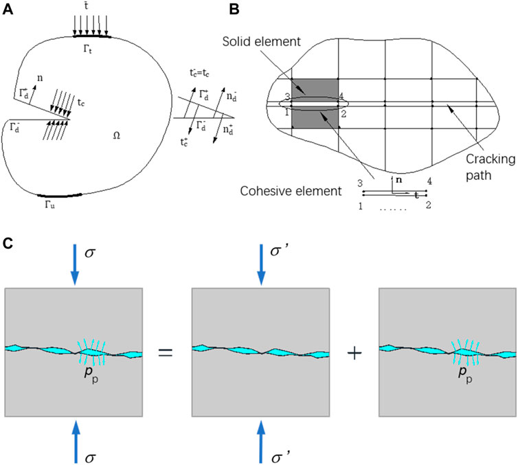
FIGURE 1. (A) Schematic diagram of cohesive element simulating cracking of rock material; (B) Schematic diagram of joint crack propagation simulated by cohesive element; (C) Schematic diagram of stress seepage coupling of joints and fissures.
The displacement field of the cohesive element can be controlled by the relative displacement of the upper and lower surfaces, and the following expression is established:
where,
Combine the relationship between the displacement field of the solid element and the node displacement. We have
where,
By combining the displacement expression of the solid element and the cohesive element, the following governing equation is established based on the weak solution form of the finite element:
where,
Combined with the stress-strain relationship of solid element and the traction separation law of cohesive element, a complete finite element solution process using the cohesive element can be established as follows:
1) Loop at the ith cohesive element under the specified loading step.
2) Obtain the node code ‘inodes’ of the ith cohesive element.
3) Obtain the degrees of freedom of the upper and lower surfaces of the ith cohesive element: idofsA and idofsB.
4) Obtain the node displacement of the upper and lower surfaces of the ith cohesive element:
5) Compute the traction displacement of the ith cohesive element.
6) Loop each Gaussian integral point by conducting the following procedure.
1) Calculate the traction displacement on the jth integral point.
#x02003; 2) Convert to local coordinate system.
#x02003; 3) Based on the traction-separation constitutive relationship, compute the bond force.
#x02003; 4) Convert the local bond force into the bond force in the global coordinate.
#x02003; 5) Calculate and update the uniform stiffness matrix of the traction-separation criterion.
7) The cohesive element’s node force and stiffness matrix are assembled into the global system to obtain the stiffness matrix and node force.
Constitutive Model for Cohesive Element
In ABAQUS, the mechanical behaviours of cohesive element are generally described using a bilinear traction-separation model [14]. In this model, the linear-growth stage before the peak-strengths describes the interfacial elastic behavior of cohesive element. It can be described by the following formula:
where
When the nominal traction stress reach the maximum values (peak-strengths)
where
When the above damage criterion is satisfied, the nominal traction stress decreases linearly, and enters the post-peak linear softening stage. A scalar damage variable
The stress components
For the linear softening, the damage evolution can be expressed as follows:
where
At the current nominal stress-strain state, the geometry area below the stress-strain curve is the normal and shear fracture energy, which can be denoted using
Where
Cohesive Element Modeling Seepage-Stress Coupling Problem
The water flow in the fractured rock mass is a typical seepage-stress coupling problem (Figure 1C). This problem is mainly manifested in three aspects.
1) The pore pressure in the fractures affects the strength and deformation of the rock mass, especially the normal deformation of the fracture. The effective stress principle can be expressed as:
where,
2) Joint void
where, unknown variables
3) Introducing the Darcy seepage formula in the cohesive element can simulate the seepage-stress coupling behaviour of rock mass. The fracture width
Models
Geological Model of Conglomerate Reservoir
The deep conglomerate reservoir is a kind of heterogeneous sedimentary rock. In terms of its geological structure, it is composed of conglomerate particles and filler matrices. When studying its material mechanical and seepage behavior, the heterogeneity of conglomerate reservoir can be simplified as a two-phase material in which conglomerate particles of different sizes are randomly embedded into the filler matrix.
Figure 2A show the plane geological model of conglomerate reservoir. It is a square area with a side length of 6000 mm. There is an initial crack extending horizontally in the middle of the left side. This initial crack penetrates the surrounding rock and extends to 200 mm in the core area of the conglomerate reservoir. The crack is used to simulate the fluid conveyance channel of hydraulic fracturing.
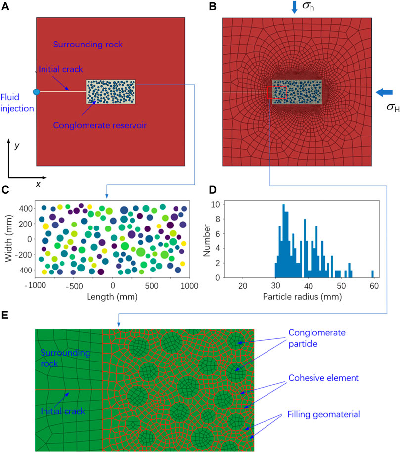
FIGURE 2. (A) Plane geological model; (B) Plane numerical model; (C) Aggregate distribution of conglomerate reservoir in the core area; (D) Statistical distribution of the aggregate size of the conglomerate reservoir in the core area; (E) An enlarged picture showing the meshes of conglomerate particles and filling geomaterial, as well as the cohesive elements embedded into the filling geomaterial.
The model size of the core stratum of the conglomerate reservoir is set to a square area of 2000 mm long and 1000 mm wide. Conglomerate aggregates are randomly generated in this area, as shown in Figure 2C. There are 129 round particles used for filling the core area. Their radius of the generated aggregates is in a range of 30–60 mm. The particle content is 30% in volume.
In the geological model of the conglomerate reservoir shown in Figure 2C, these aggregates are divided into six groups using different colors according to size. Figure 2D performs a statistical analysis on the geometric dimensions of the generated 129 aggregates. It can be seen that most conglomerate particles are concentrated in the size range of 30–45 mm.
Numerical Model of Conglomerate Reservoir
The problem concerned in this study is simplified to a plane strain problem to be solved using ABAQUS. The first-order linear plane strain quadrilateral element is used to mesh the geological model. Then, a numerical model is obtained, as shown in Figure 2B. The numerical model has 8,895 plane strain quadrilateral elements and 8,927 nodes.
This study uses the cohesive element to simulate the conglomerate reservoir’s discontinuous deformation and failure under hydraulic fracturing loads. We consider that the conglomerate aggregates do not fail and the hydraulic fracturing cracks only occur inside the filler. Therefore, the cohesive elements are only embedded within the plane strain elements of the filler of the conglomerate reservoir. Figure 2E shows the numerical calculation model after embedding the cohesive elements. This new model has a total of 9,226 cohesive elements.
Loads and Boundary Conditions
The model’s left side is the symmetrical plane, which is an impervious boundary. The midpoint of the initial fracture on the left side is the fluid injection point (Figure 2A). In calculation, the mechanical boundary condition at this point is the pore pressure of hydraulic fracturing. The nodal displacements in the x-axis and y-axis directions of the four edges around the model are constrained.
All of the nodes in the model are set as constant pore pressure conditions. The initial pore pressure of these nodes is set to 0 MPa, and the initial void ratio is set as
As shown in Figure 2B, the horizontal minor principal in-situ stress
Mechanical Parameters
In this numerical model, four types of geomaterials are involved: surrounding rocks, conglomerate aggregates, fillers, and cohesive interfaces around the aggregates. The material parameters used in the numerical simulations are given in Table 1.
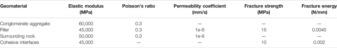
TABLE 1. Mechanical parameters of the geomaterials used in the numerical simulations.
Implementation of Temporary Plugging Simulation
The numerical modeling of the temporary plugging treatment in the rock mass is difficult in FEM simulations. In order to realize this modeling in ABAQUS, an available method is by reading the crack propagation data of the cohesive elements and increasing the fluid’s dynamic viscosity in these positions.
In actual execution, the coordinates of the crack tips in the cohesive elements at the temporary plugging moment can be recorded. Then, a USDFLD subroutine (user-defined field variable) is called by ABAQUS to increase the liquid flow’s dynamic viscosity in these cohesive elements in the subsequent calculations. Thereby, an increase in the fluid’s resistance passing through these cohesive elements would force the initiation and propagation of new branch fractures in other locations with lower resistance.
The calculation time lasts to 21 s, divided into two stages. 1) During the period of t = 0–1 s, the pore pressure increases sharply at the fluid injection point from 0 to 10 MPa. 2) During the period of t = 1–8 s, the increased pore pressure leads to the first splitting crack propagation at the tip of the fracture. 3) Starting from t = 8 s, at the forefront of the formed hydraulic fractures, temporary plugging is conducted by changing the value of dynamic viscosity of the fluid at the cracking cohesive elements. The blocking length is set to 100 mm.
Modelling Results and Analysis
Fracturing Characteristics
Figure 3 shows the expansion and distribution of the fractures induced by temporary pugging-refracturing in the conglomerate reservoir under four in-situ stress differences. It can be seen that the fractures caused by hydraulic fracturing in the conglomerate reservoir propagate along the initial fracture and the direction of the major principal in-situ stress.
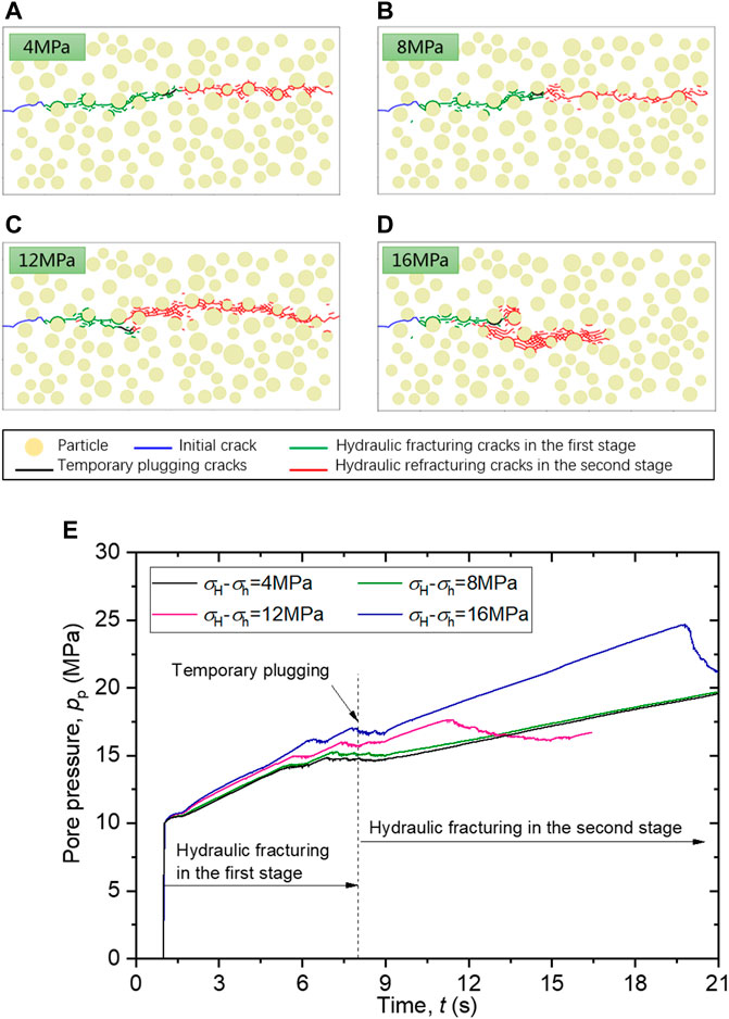
FIGURE 3. (A,B,C,D) Fracture evolution characteristics of temporary plugging-refracturing under different in-situ stress differences; (E) Pore pressure history curve at injection point under different horizontal stress difference.
When the in-situ stress difference is relatively smaller, that is
Figures 3C,D shows the expansion and distribution of the fractures in the conglomerate reservoir under higher horizontal stress difference conditions, i.e.,
It is observed from Figure 3D that, when
Evolution of Pore Pressure
Figure 3E shows the pore pressure changes with time at the fluid injection point. In general, with the increase of the major principal in-situ stress
When time exceeds 6 s, the pore pressures at the fluid injection point enter relatively flat plateaus under the four in-situ stress conditions. The conglomerate reservoir was hydraulically fractured at these flat plateaus of the pore pressures. Because of the initiation and propagation of the fractures, the fracture volumes increase, making it difficult for the pore pressure at the fluid injection point to increase continuously.
When time = 8 s, the cracks produced by the first hydraulic fracturing are temporarily blocked. After the temporary plugging treatment, for the case of
In the case of
For the case of
Conclusions
In this study, ABAQUS is used to numerically simulate the temporary plugging-refracturing process in the conglomerate reservoir under four in-situ stress states. The following conclusions can be summarised:
1) In FEM analysis, the cohesive element can effectively simulate the discontinuous deformation and failure of the rock mass. Furthermore, the cohesive element containing the constitutive relationship of Darcy seepage is capable of simulating the seepage-stress coupling behaviour of the fractured rock mass.
2) In this study, by reading the data of crack propagation, the cracked cohesive elements are identified. A USDFLD subroutine is used to increase the dynamic viscosity of the liquid flow in these cracked cohesive elements. The numerical simulation of plugging treatment is successfully realized.
3) While under higher horizontal in-situ stress difference, it is easier to generate new branch fractures to bypass the temporary plugging position. With the increase of in-situ stress difference, the more complex the branch fractures and the higher the pore pressure used for hydraulic fracturing the conglomerate reservoir.
4) During temporary plugging-refracturing process, pore pressure distribution and fracture propagation can be observed. By analyzing the pore pressure-time history curve of the fluid injection point, the hydraulic fracturing events in the conglomerate reservoir can be judged.
5) The numerical simulation results obtained in this study are relatively intuitive, but the model of the conglomerate reservoir is somewhat different from the actual geological condition. When the actual engineering geological conditions are clear and there are accurate calculation parameters, the work carried out in this research can provide effective and reasonable suggestions for the actual petroleum engineering.
Data Availability Statement
The raw data supporting the conclusion of this article will be made available by the authors, without undue reservation.
Author Contributions
Numerical simulations were contributed by JC and JZ. Programming the USDFLD subroutine was mainly contributed by QZ. Drafting the manuscript was contributed by JC and JZ.
Funding
This research was financially supported by the Open Research Fund of Key Laboratory of Construction and Safety of Water Engineering of the Ministry of Water Resources, China Institute of Water Resources and Hydropower Research (Grant No. 202101) and by National Natural Science Foundation of China (Grant No. 12062026).
Conflict of Interest
JC is employed by Sany Heavy Industry Co. Ltd.
The remaining authors declare that the research was conducted in the absence of any commercial or financial relationships that could be construed as a potential conflict of interest.
Publisher’s Note
All claims expressed in this article are solely those of the authors and do not necessarily represent those of their affiliated organizations, or those of the publisher, the editors and the reviewers. Any product that may be evaluated in this article, or claim that may be made by its manufacturer, is not guaranteed or endorsed by the publisher.
References
1. Bakhshi E, Golsanami N, Chen L. Numerical Modeling and Lattice Method for Characterizing Hydraulic Fracture Propagation: A Review of the Numerical, Experimental, and Field Studies. Arch Computat Methods Eng (2021) 28:3329–60. doi:10.1007/s11831-020-09501-6
2. Zhang R, Hou B, Tan P, Muhadasi Y, Fu W, Dong X, et al. Hydraulic Fracture Propagation Behavior and Diversion Characteristic in Shale Formation by Temporary Plugging Fracturing. J Pet Sci Eng (2020) 190:107063. doi:10.1016/j.petrol.2020.107063
3. Wang B, Zhou F, Wang D, Liang T, Yuan L, Hu J. Numerical Simulation on Near-Wellbore Temporary Plugging and Diverting during Refracturing Using XFEM-Based CZM. J Nat Gas Sci Eng (2018) 55:368–81. doi:10.1016/j.jngse.2018.05.009
4. Chen W, Konietzky H, Liu C, Tan X. Hydraulic Fracturing Simulation for Heterogeneous Granite by Discrete Element Method. Comput Geotechnics (2018) 95:1–15. doi:10.1016/j.compgeo.2017.11.016
5. Nagel NB, Sanchez-Nagel MA, Zhang F, Garcia X, Lee B. Coupled Numerical Evaluations of the Geomechanical Interactions Between a Hydraulic Fracture Stimulation and a Natural Fracture System in Shale Formations. Rock Mech Rock Eng (2013) 46:581–609. doi:10.1007/s00603-013-0391-x
6. Zou Y, Zhang S, Ma X, Zhou T, Zeng B. Numerical Investigation of Hydraulic Fracture Network Propagation in Naturally Fractured Shale Formations. J Struct Geology (2016) 84:1–13. doi:10.1016/j.jsg.2016.01.004
7. Deng J, Yang Q, Liu Y, Liu Y, Zhang G. 3D Finite Element Modeling of Directional Hydraulic Fracturing Based on Deformation Reinforcement Theory. Comput Geotechnics (2018) 94:118–33. doi:10.1016/j.compgeo.2017.09.002
8. Dong Y, Tian W, Li P, Zeng B, Lu D. Numerical Investigation of Complex Hydraulic Fracture Network in Naturally Fractured Reservoirs Based on the XFEM. J Nat Gas Sci Eng (2021) 96:104272. doi:10.1016/j.jngse.2021.104272
9. Cai X, Liu W, Shen X, Gao Y. Flow-coupled Cohesive Interface Framework for Simulating Heterogeneous Crack Morphology and Resolving Numerical Divergence in Hydraulic Fracture. Extreme Mech Lett (2021) 45:101281. doi:10.1016/j.eml.2021.101281
10. Li J, Dong S, Hua W, Li X, Guo T. Numerical Simulation of Temporarily Plugging Staged Fracturing (TPSF) Based on Cohesive Zone Method. Comput Geotechnics (2020) 121:103453. doi:10.1016/j.compgeo.2020.103453
11. Nguyen VP, Lian H, Rabczuk T, Bordas S. Modelling Hydraulic Fractures in Porous media Using Flow Cohesive Interface Elements. Eng Geology (2017) 225:68–82. doi:10.1016/j.enggeo.2017.04.010
12. Barenblatt GI. The Formation of Equilibrium Cracks during Brittle Fracture. General Ideas and Hypotheses. Axially-Symmetric Cracks. J Appl Mathematics Mech (1959) 23:622–36. doi:10.1016/0021-8928(59)90157-1
13. Dugdale DS. Yielding of Steel Sheets Containing Slits. J Mech Phys Sol (1960) 8:100–4. doi:10.1016/0022-5096(60)90013-2
Keywords: conglomerate reservoir, temporary plugging, hydraulic fracturing, numerical simulation, cohesive element
Citation: Chen J, Zhang Q and Zhang J (2022) Numerical Simulations of Temporary Plugging-Refracturing Processes in a Conglomerate Reservoir Under Various In-Situ Stress Difference Conditions. Front. Phys. 9:826605. doi: 10.3389/fphy.2021.826605
Received: 01 December 2021; Accepted: 20 December 2021;
Published: 27 January 2022.
Edited by:
Qingxiang Meng, Hohai University, ChinaReviewed by:
Shiyue Zhang, Shanghai Research Institute of Materials (SRIM), ChinaLanlan Yang, Jiangnan University, China
Copyright © 2022 Chen, Zhang and Zhang. This is an open-access article distributed under the terms of the Creative Commons Attribution License (CC BY). The use, distribution or reproduction in other forums is permitted, provided the original author(s) and the copyright owner(s) are credited and that the original publication in this journal is cited, in accordance with accepted academic practice. No use, distribution or reproduction is permitted which does not comply with these terms.
*Correspondence: Jiuchang Zhang, emhhbmdqaXVjaGFuZ0Bmb3htYWlsLmNvbQ==