 Isabella Petrelli1†
 Francesca Santoro1†
 Gianlorenzo Massaro2,3*
 Francesco Scattarella2,3
 Francesco V. Pepe2,3Francesca Mazzia4Maria Ieronymaki5George Filios5Dimitris Mylonas5Nikos Pappas5
 Cristoforo Abbattista1‡
 Milena D’Angelo2,3‡
- 1Planetek Italia s.r.l. (Italy), Bari, Italy
- 2Dipartimento Interuniversitario di Fisica, Università degli Studi di Bari, Bari, Italy
- 3Istituto Nazionale di Fisica Nucleare, Bari, Italy
- 4Dipartimento di Informatica, Università degli studi di Bari, Bari, Italy
- 5Planetek Hellas E.P.E., Marousi, Greece
Correlation Plenoptic Imaging (CPI) is an innovative approach to plenoptic imaging that tackles the inherent trade-off between image resolution and depth of field. By exploiting the intensity correlations that characterize specific states of light, it extracts information of the captured light direction, enabling the reconstruction of images with increased depth of field while preserving resolution. We describe a novel reconstruction algorithm, relying on compressive sensing (CS) techniques based on the discrete cosine transform and on gradients, used in order to reconstruct CPI images with a reduced number of frames. We validate the algorithm using simulated data and demonstrate that CS-based reconstruction techniques can achieve high-quality images with smaller acquisition times, thus facilitating the practical application of CPI.
1 Introduction
Correlation Plenoptic Imaging (CPI) [1–9], is a recently developed approach to plenoptic imaging (also know as light-field imaging), which aims, by exploiting correlations of light intensity, to overcome the strong tradeoff between image resolution and maximum achievable depth of field that affects conventional techniques, based on direct intensity measurements [10–18]. All plenoptic imaging techniques aim at reconstructing the three-dimensional distribution of light in a scene by simultaneously encoding in optically measurable quantities information on the intensity and the distribution of light in given reference plane in the scene. Detection of the propagation direction of light offers several advantages compared to conventional imaging, since it provides high-depth-of-field images of the sample from different perspectives, thus enabling post-acquisition volumetric refocusing without the need for scanning the scene of interest. While in conventional PI spatial and directional information are encoded, usually by means of a microlens array, in the intensity impinging on a single sensor, in CPI they can be retrieved only by measuring spatio-temporal correlations between intensities registered by pixels on two disjoint sensors. In fact, the initial embodiments of CPI [1] were inspired by a previously established correlation imaging technique, called Ghost Imaging (GI): here, a two-dimensional image is obtained by correlating the total intensity transmitted (or reflected) by an object, as measured through a single-pixel (known as bucket) detector, with the signal acquired by a sensor with high spatial resolution that, conversely, collects light that has not interacted with the object [19–26]. The main difference between GI and CPI lies in the much larger amount of information collected by measuring light correlations on two space-resolving sensors, compared with the single-pixel measurement performed in GI. In GI, in fact, the object can be successfully reconstructed only when it is at focus, whereas CPI can refocus the image over a much larger axial depth.
Despite their promising application potentials, CPI and GI share the main drawback of correlation imaging techniques, namely, the need to accumulate statistics (i.e., independent intensity frames) in order to reconstruct the desired correlation signal. In particular, the signal-to-noise ratio (SNR) of CPI and GI images scales like the square root of the number of acquired frames [27–29], but the acquisition time increases linearly in the latter quantity, leading to a necessary compromise between accurate and fast imaging. In the case of GI, many efforts have been made to reduce the sampling rate and enhance the acquisition speed without sacrificing the image quality. Interesting attempts to model the problem of image reconstruction as an optimization problem, following the principles of compressive sensing (CS), have been successfully applied to increase image quality in case of scarce statistics [30,31]. The basic idea behind CS is to employ only a few samples and exploit the sparsity of the acquired signal in some specific domain to reconstructing a high-SNR image [32–35]. From the theoretical point of view, CS is a convex optimization problem, in which one looks for the sparsest signal that minimizes a given cost function. As detailed in the following sections, the choice of a cost function to optimize depends both on the structure of the problem to be faced, and on specific requirements in the reconstructed image (e.g., weighing data-fidelity or sparsity terms, or considering additional noise-related effects).
In this paper, we investigate the feasibility of applying CS inspired techniques to CPI, building on the promising results achieved in compressive GI. We propose a CS-based algorithm that incorporates a regularization term which exploits the sparseness of image gradients as an alternative approach with respect to the conventional correlation-based one. The algorithm, specifically designed for Correlation Plenoptic Imaging, aims at 1) reducing the number of frames necessary to achieve a target image quality, 2) replacing the CPI cross-correlation computation with an optimization process. The paper is organized as follows: in Section 2.1, we recall the basic concepts of Correlation Plenoptic Imaging; in Section 2.2, we introduce a formal description of the proposed CS-based algorithm for CPI reconstruction; in Section 3, the proposed method is investigated numerically; we summarize the results and provide final remarks in Section 4.
2 Materials and methods
2.1 Fundamentals of correlation plenoptic imaging
The CPI technique extends the potentials of GI by enabling one to retrieve combined spatial and directional information without scanning the scene. CPI substantially differs from GI in the fact that both the detectors that register the intensities to be correlated are characterized by spatial resolution. Such a feature has a relevant implication in the evaluation of correlations, as we are going to explain in the following. Though the results obtained in this work can be generalized to any CPI setup, we refer for the sake of definiteness to the setup that bears the closest analogy to GI, namely, the first one to be proposed [1] and experimentally realized [3], schematically depicted in Figure 1.
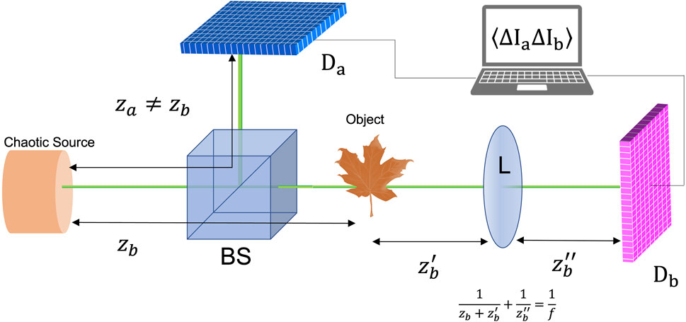
FIGURE 1. Scheme of the setup employed for the first demonstration of CPI [1,3]. A lens L in interposed in the arm in which the object is located, to obtain an image of the chaotic source on the spatially-resolving detector Db. By measuring second-order intensity correlations, a collection of images of the object can be retrieved in correspondence of the other spatially-resolving detector Da, one for each pixel of Db.
We consider a source emitting quasi-monochromatic light with chaotic (pseudothermal) statistics, characterized by negligible spatial coherence on its emission surface; the source is divided in two paths by a beam splitter. One of the beams (the reflected one, in the case depicted in Figure 1) follows path a and directly reaches the detector Da, which is located at an optical distance za from the source, without interacting with the object. The other beam (the transmitted one in Figure 1) follows path b, where it first interacts with a sample, placed at a distance zb from the source, and considered for simplicity as a planar transmissive object; then, it passes through a lens L of focal length f, placed at a distance
The correlation of the intensity fluctuations measured by the two detectors can be expressed by the following formula:
where ρa and ρb are the planar coordinates of pixels on detector Da and Db, respectively, while ΔIa and ΔIb are the temporal intensity fluctuations recorded on the pixels specified in their arguments. The statistical average ⟨… ⟩ can be reconstructed by collecting M frames, in which the object is illuminated by independent chaotic (speckle) patterns. Eq. 1 shows the main difference between GI and CPI: in fact, whereas ghost imaging retrieves the image of the object by measuring correlations between Da and a bucket detector, CPI makes use of the additional information originating from the spatial resolution of Db to refocus. In other terms, CPI would reduce to GI if Db were composed by a single-pixel detector. Applying the geometrical optics approximation, the correlation function can be expressed in terms of the intensity profile of the chaotic source
Therefore, in the geometrical approximation, the correlation function, which is defined in the 4D space of the detector coordinates, reduces to the product of the image of the source, as retrieved by Db, with images of the object calculated as a function of a linear combination of the coordinates on both detectors. As anticipated, in fact, each image obtained by fixing a value for ρb corresponds to an image of the object, scaled and shifted according to the chosen value of ρb and the coefficients of the linear combination. When the object is placed in zb = za, as is the case in conventional GI, the sub-images are neither shifted nor rescaled from one another, and integration over ρb (i.e., sum of all sub-images) gives the standard ghost image. However, this operation provides a focused image only when za = zb (more precisely, when the difference of the two distances is smaller than the depth of field defined by the light wavelength and the source numerical aperture, as seen from the object plane [1,3]). The situation changes if the object is displaced of an arbitrary quantity from the focused plane. In this case, the operation of integrating the Γ function over ρb to obtain a ghost image as in the previous case is detrimental. This because being
provides, in the geometrical optics limit, a faithful image of the object, regardless of its position. In fact, as one can easily check, if the coordinate transformation on the first argument of Γ is applied on Eq. 2, the ρb-dependence is conveniently lost. Finite wavelenghts, instead, set limits related to wave optics [3]. It is worth noticing that, in order to get a properly refocused image, one should know with sufficient precision both the source-to-Da distance za and the source-to-object distance zb. However, a likely situation is the one in which za is precisely determined by the choice of the experimental setup, while the value of zb is unknown: in this case, the parameter zb in Eq. 3 can be adjusted in order to maximize sharpness of the refocused image, thus also providing a way to estimate of the object distance.
The extension to CPI of the CS-based reconstruction algorithms designed for chaotic GI [30,31] is not trivial. The main difference lies precisely in the presence of the linear transformation 3) to be applied to the correlation function, and the subsequent integration over the “directional” detector Db. These algorithms rely on the minimization of an objective function, whose formulation must incorporate in a proper way the linear transformation of the Γ function in the aforementioned equation.
2.2 Compressive correlation plenoptic imaging
Since the application of CS to CPI can be considered as a generalization of its application to GI, we employ a notation that makes the parallelism between the two imaging techniques more evident. After defining as
the corresponding intensity fluctuation, where the second term is an estimate of the mean intensity. The correlation function Γ, estimated after collecting m frames, thus reads
As already mentioned, the term
with
Similarly, the M × 1 measurement vector corresponding to the ith pixel in position (xb, yb) is obtained by stacking all the bucket signals
Notice that while the measurement vectors depend on the particular pixel of Db under analysis, the measurement matrix is independent of such pixels. Therefore, the measurement process imposes a generally different matrix constraint on each out-of-focus image. If we indicate with γi the flattened version of
In principle, at least
Before defining the objective function, and therefore the complete minimization problem to be tackled, it is worth noticing that the latter must keep track of the refocusing process 3), leading to the target image on which prior knowledge exists. On the other hand, constraints are formulated in terms of the out-of-focus images. Refocusing cannot be reduced to a matrix multiplication, and depends on the coordinate of pixels on the detector Db. To solve this issue and recast the problem into a more tractable one, we reverse the standard workflow. Since refocusing amounts to a reassigning the coordinates on detector Da based on the values of (xb, yb), we perform such a remapping on top of the cross-correlation step that we aim to replace. We start by defining the “refocused Γ” as
with
The updated workflow leads to a refactoring of the constraints encoding the measurements. In particular, Eq. 9 is replaced by
where the
The CS formulation in terms of an optimization problem, for which efficient algorithms exist, involves the minimization of an objective function given by the sum of two terms: a data fidelity term, encoding the constraints, and a regularization term, which expresses prior information of the object to be detected. The solution of the problem, representing the optimal reconstructed image, reads
with
with L operator performing the transform in the domain where the image is supposed to be sparse. The above optimization problem can be recast in terms of the image transform
with
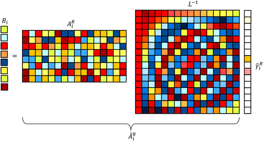
FIGURE 2. Graphical representation of the CS optimization procedure defined by Eq. 15.
Many established CS reconstruction algorithms exploit the prior knowledge that natural images are sparse in a given domain, such as discrete cosine transform (DCT) (see Ref. [30] for an application to GI). However, image signals are usually reshaped into one-dimensional signals, thus hiding part of the structure information. In this context, we explore a regularization term related to the total variation (TV) of the image, namely, the norm of the image gradient. CS-based TV regularization methods exploit the sparseness of the image gradients in the spatial domain. More complex solutions include more than one regularization term, promoting both sparsity of DCT or Fourier transform and image gradients. Possible regularization strategies involve the functions outlined below:
• Case 1: sparse structure is expected in a transform domain such as the DCT. The inverse transform matrix represents the 2D inverse DCT, applied to the minimization outcome to obtain the reconstructed two-dimensional image
• Case 2a: as well-known from previous works [39–41], the discrete gradient of natural images along the horizontal and vertical directions are sparse, therefore TV regularization can be used, as firstly proposed by Rudin-Osher-Fatemi [42]. While the original formulation is referred to as the isotropic total variation, an anisotropic formulation was also addressed in the literature [43],
Where Dx and Dy denote the horizontal and vertical discrete partial derivatives, respectively, and D = (Dx, Dy) is the discrete gradient operator. The discrete partial derivatives are approximated by first order forward differences. From the numerical point of view, the exact total variation term can make the problem intractable. However, after some manipulations, it is possible to recast the optimization problem which includes the anisotropic approximation of the TV term to the standard form by means of an extended model, with
• Case 2b: other edge-detection operators were considered in previous research [44], such as the Laplacian operator
The reason why we consider a second-order regularization term is due to the fact that the problem can be easily recast to a standard form without extending the model, but just considering the modified sensing matrix
The previously described regularization terms can be combined with each other (here, we limit our analysis to the anisotropic approximation of the TV and to the Laplace operator), at the expense of the computational complexity. The reason is twofold: the optimal choice of the regularization parameters is usually a non-trivial task, and recasting it to the standard form, for which efficient solvers exist, is possible only by extending the model.
There is one final element to consider regarding the shape of the objective function. Thus far, we have formulated
The multiple-problems approach adheres more closely to the original workflow, where each distinct perspective or refocused image (corresponding to individual pixels of Db) is reconstructed independently: through correlation in the original approach, solving a minimization problem in the CS-based one. Subsequently, these
On the other hand, the single-problem formulation exploits the fundamental insight that, once the sensing matrix is refocused a priori, we are effectively striving to reconstruct the same object image from multiple viewpoints. This observation enables us to join the various optimization problems by merging the sensing matrices, as well as the corresponding bucket measurements. From an implementation standpoint, this means stacking all the refocused measurement matrices and all the measurement vectors: a graphical explanation is provided in Figure 3. Consequently, the single-problem approach entails solving one optimization problem, with the objective of obtaining the sparsest image,
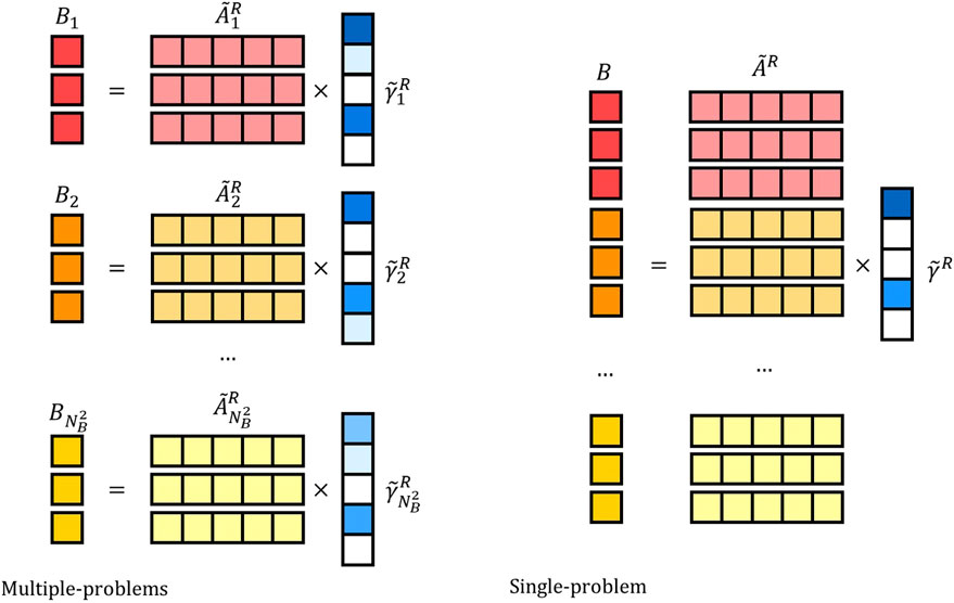
FIGURE 3. Graphical representation of two approaches to objective function minimization. Left: multiple-problems formulation. Right: single-problem formulation. In the multiple-problems formulation, we solve
However, it is worth recognizing that the single-problem formulation comes with a challenge: The stacking of several sensing matrices and associated measurements vectors leads to the creation of large matrices, which, in turn, increases the computational complexity. Ultimately, the choice between the multiple-problems and single-problem formulations should be the result of a trade-off between computational complexity and reconstruction quality.
3 Numerical results
The multiple-problems and single-problem strategies are tested on simulated datasets accounting for source statistics and field propagation. The CS-CPI algorithm was implemented in Python. Specifically, we utilized the scikit-learn library, whose modules encompasses a variety of linear models, including Lasso [45]. The standard reconstruction obtained by correlating a large number of frames (N = 15,000) is taken as the ground truth, a random subset of M frames is extracted from the collection to test CS procedures. To quantify the size of the subset, we consider two parameters: the total number of measurements over the total number of “spatial” pixels,
The chosen quality metric is the Structural SIMilarity (SSIM) index [46]. Consider x and y two non-negative image signals. If x is supposed to be the reference with perfect quality, then the similarity measure is a quantitative measurement of the quality of the second signal. In this context, the SSIM is defined as
where the similarity measurement is split into three comparisons: luminance l (x, y), contrast c (x, y) and structure s (x, y). The three functions are defined as
The constants
The definition above satisfies the following conditions:
• Simmetry: SSIM(x, y) = SSIM(y, x),
• Boundedness: SSIM(x, y) ≤ 1,
• Unique maximum: SSIM(x, y) = 1 if and only if x = y.
Finally, the exponents ω > 0, ϕ > 0 and ψ > 0 are parameters used to adjust the relative importance of the three components. In the following, we set ω = ϕ = ψ = 1 and C3 = C2/2, K1 = 0.01 and K3 = 0.03.3.1 Case 1: Sparsity in the DCT domain
Since natural images tend to be compressible in the DCT domain, we solve the minimization problem encoded in Eq. 15 using standard convex programming algorithms (e.g., the coordinate descent algorithm). Multiple-problems and single-problem strategies have both been tested. A random sample of M = 225 frames, corresponding to α = 0.05, is extracted and used for the reconstruction. Following this approach, the CS-CPI algorithm improves the reconstruction quality, as highlighted by the results reported in Figure 4. The left panel reports the value of the structural similarity index as a function of the regularization parameter in the CS-CPI case, compared with the value of the correlation in the standard case. Panels on the right compares the reconstruction obtained through cross-correlation with the results obtained with the CS-CPI algorithm, for different values of the parameter λ.
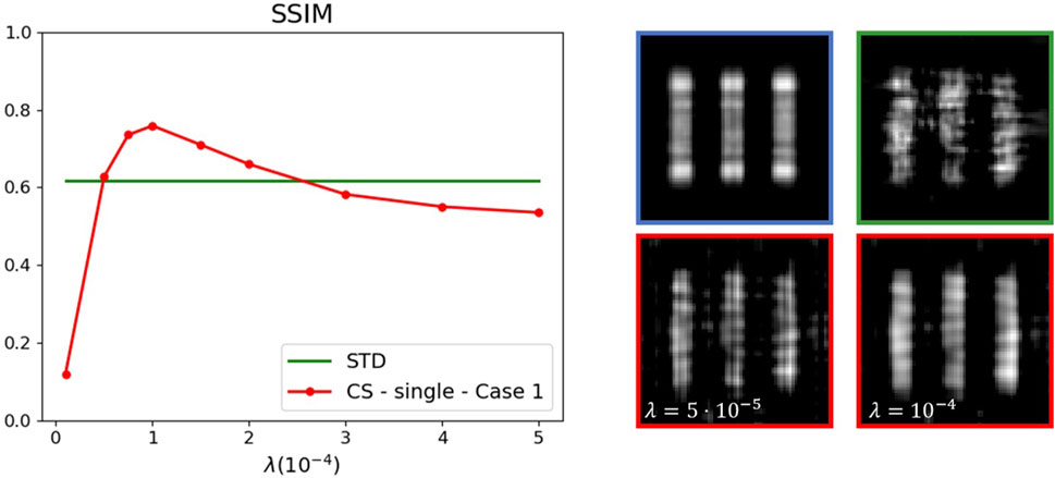
FIGURE 4. CS-CPI algorithm (single-problem formulation, Case 1 regularization) applied on a simulated dataset (blue box, standard reconstruction with all frames). The proposed CS-CPI algorithm (red boxes/curve) can overcome the standard correlation evaluation with the same number of frames (green box/curve) in a range of regularization parameter values.
This strategy entails an obvious drawback: huge matrices are involved in the minimization problem, with
The performance of the multiple-problems strategy is not as good as the single-problem one, as expected. The resulting image quality of the two procedures becomes comparable by doubling the frames used for the multiple problems (α = 0.1). As shown in Figure 5, the CS-CPI reconstruction is always poorer than the one obtained through the standard correlation-based evaluation with the same number of frames, except for a narrow range of parameters within which the quality of the two reconstructions become comparable.
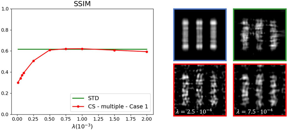
FIGURE 5. CS-CPI algorithm (multiple-problem formulation, Case 1 regularization) applied on a simulated dataset (blue box, standard reconstruction with all frames). Even if the proposed CS-CPI algorithm (red boxes/curve) is able to reconstruct the image, the quality of the standard correlation evaluation (green box/curve) with the same number of frames is always better, except for a narrow range of parameters within which the reconstructions become comparable.
In the context of CS, the regularization parameter optimization is a challenging task due to the need for prior knowledge of ideal outcomes. The most suitable parameter is greatly influenced by both the observation model and the specific subject of interest. Consequently, there is no universally applicable method for fine-tuning regularization parameters.
The regularization parameter λ, a trade-off between sparsity and data fidelity, is expected to affect the quality of the image reconstruction Yang et al. [47]. The numerical experiments conducted to assess the sensitivity of λ on the reconstructed image quality (whose results are encoded in Figures 4, 5) show that an optimal λ value exists that yields the best performance in image reconstruction.From Eq. 15, which encapsulates the essential trade-off in CS, the first term primarily serves the purpose of fitting the measured data to reconstruct the image vector, whereas the secon term controls its degree of sparsity. A larger λ places more emphasis on enforcing sparsity within the object, effectively suppressing unsparse image noise. Conversely, a smaller λ has the opposite effect, allowing for the preservation of finer details of the object.
Generally, it is not granted that the CS-based reconstruction outperforms the standard one. The performance of CS algorithms depend on several factors including the properties of the measurement matrix, excessive noise in the measurements, convergence issues in the optimization algorithm or spurious correlations in the measurement matrix.
3.2 Case 2: Sparsity in the gradient domain
As discussed in Section 2.2, we tested a version of the CS-based reconstruction algorithm for CPI that incorporates sparsity of image gradients as a regularization term. Specifically, we considered the anisotropic TV approximation (Case 2a) and the Laplacian (Case 2b). Furthermore, we explored the combination of regularization terms, imposing sparsity on both the DCT and the gradients. Also in this context, we tested both the single-problem and multiple-problems strategies. The same random sample of M = 225 frames, corresponding to α = 0.05, used in Case 1 was also used in this second case and employed for the reconstruction. However, the performance of the reconstruction algorithm in case 2a (anisotropic approximation of the TV term with and without the DCT term) is not satisfying, hence the results are not shown. In particular, in order to obtain a sufficiently good reconstruction (in any case worse than that obtained by correlations), it is necessary to increase the number of frames by at least 3 times. Thereby, in the rest of this paragraph we will concentrate on case 2b. The best image reconstructions in the four cases described above are reported in Figure 6, see the caption for details on the parameters values.
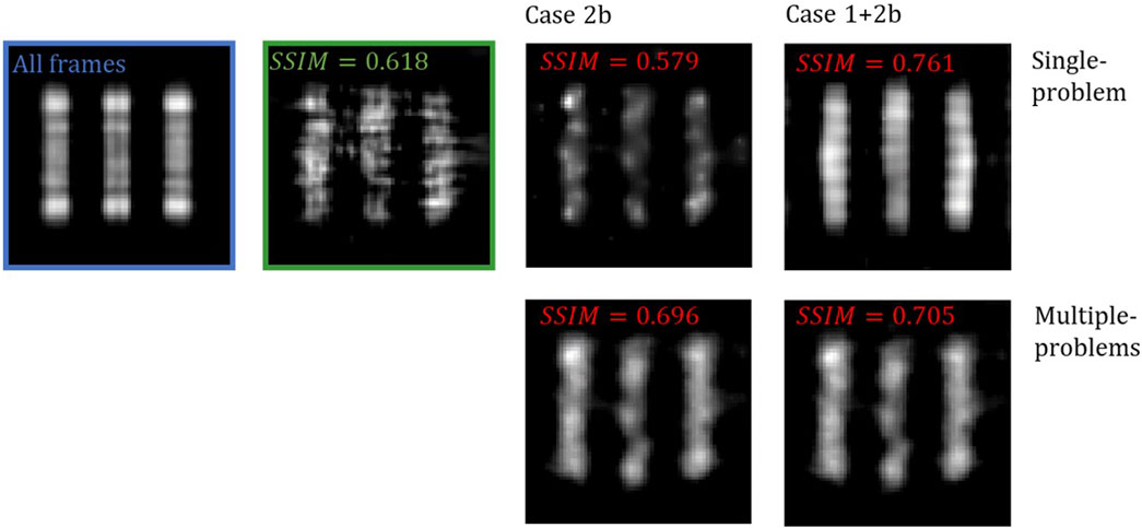
FIGURE 6. CS-CPI algorithm results (first row: single-problem formulation, second row: multiple-problems formulation. Case 2b with and without DCT regularization). The proposed CS-CPI algorithms can overcome the standard correlation evaluation with the same number of frames (green box) in all cases except Case 2b (single-problem formulation), as evident from the structural similarity index reported in the images. The regularization parameters used for the reconstruction are: λ =2.5⋅10−5 (single-problem Case 2b), λ =5⋅10−5, γ =2.5⋅10−4 (single-problem, Case 1+2b), λ =5⋅10−4 (multiple-problems, Case 2b), λ =5⋅10−4, γ =2.5⋅10−4 (multiple-problems, Case 1+2b). (SSIM values in figure updated).
As evident from Figures 7, 8, all the versions of the CS-CPI algorithm with single-problem and multiple-problems approaches improve image quality (except for Case 2b in the single-problem formulation whose results are comparable with the standard correlation case) with the Case 1+2b (single-problem formulation) giving the best results in terms of reconstruction quality.
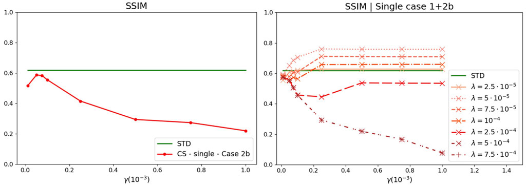
FIGURE 7. CS-CPI algorithm (single-problem formulation, left: Case 2b, right: Case 1+2b regularizations) applied on a simulated dataset. This version of the proposed CS-CPI algorithm succeeds in the reconstruction if both regularization terms are included in a certain range of the regularization parameters λ and γ.
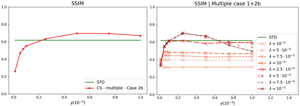
FIGURE 8. CS-CPI algorithm (multiple-problems formulation, left: Case 2b, right: Case 1+2b regularizations) applied on a simulated dataset. This version of the proposed CS-CPI algorithm guarantees a good image reconstruction in both cases (with and without the DCT regularization term) with minimal differences.
Comparing the results reported in Figure 4 with Figure 7, as well as the results from Figure 5 with Figure 8, it emerges that the introduction of a regularization term requiring gradient sparsity enhances reconstruction quality, since it tends to penalize fast noise fluctuations in the background, limiting at the same time the introduction of artifacts. Reconstruction capability is further enhanced when the requests of sparsity in the gradient and the transform domains are combined. In particular, the most promising results are observed in Case 1+2b (single-problem formulation). However, it is worth noticing that the single-problem formulation of the CS-CPI algorithms provides satisfactory results also in its simpler formulation (Case 1). Instead, when analyzing the results of the multiple-problems strategy, the presence of a term penalizing the image gradients seems crucial. Actually, while the multiple-problems approach to CS-CPI is not able to provide a satisfactory reconstruction, as shown in Figure 5, introducing a TV-related term (the image Laplacian) reverses the situation. From an overall comparison involving single- or multiple-problems strategies, as well as all the considered regularization term, it emerges that the best results are obtained when both the DCT and the Laplacian of the target image are regularized.
We conclude by showing in Figure 9 the average pixel value along the slit direction and across them. The contrast obtained in the CS-TV case, corresponding to the multiple-problems formulation with the DCT and the Laplacian regularization terms, is always higher than in the correlation-based reconstruction obtained with the same frame subset, while it is comparable with the correlation-based ground truth, obtained with all the available frames.
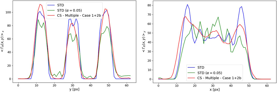
FIGURE 9. Average pixel value along the slits direction (left panel) and across them (right panel). The blue line corresponds to the standard reconstruction with all frames, the green one to the standard with a reduced frame subset and the red line to the CS-CPI result (multiple-problems formulation, case 1+2b). The parameters are the same as in Figure 6.
4 Conclusion
CPI is a novel technique capable of acquiring the light field, the combined information of intensity and propagation direction of light. The standard image retrieval is performed by evaluating correlations between the intensities measured by two detectors with spatial resolution. In this work, we have discussed a first demonstration of the applicability of CS-based approaches to CPI. We have explored several possibilities for building the objective function. Specifically, we have tested two approaches: one envisaging a single-problem formulation, in which the whole information on the object coming from all light propagation directions is exploited at once, and the other a multi-problem approach, in which reconstruction is separately performed for the object illuminated by different source points. Besides, we have considered regularization terms promoting both the sparsity of the image DCT and the sparsity of the image gradient, showing that, at a fixed frame number, CS-based approaches can boost the CPI image quality with respect to the deterministic correlation measurement, thus allowing for shorter acquisition times. Nevertheless, the high computational costs usually associated with common CS implementations still represent a bottleneck towards the extensive application of the selected solution into the operational CPI framework.
Data availability statement
The raw data supporting the conclusion of this article will be made available by the authors, without undue reservation.
Author contributions
IP: Conceptualization, Formal Analysis, Methodology, Software, Writing–original draft, Writing–review and editing. FSa: Conceptualization, Software, Writing–review and editing. GM: Data curation, Software, Writing–review and editing. FSc: Writing–original draft, Writing–review and editing. FP: Conceptualization, Writing–original draft, Writing–review and editing. FM: Conceptualization, Methodology, Writing–review and editing. MI: Funding acquisition, Writing–review and editing. GF: Validation, Writing–review and editing. DM: Validation, Writing–review and editing. NP: Validation, Writing–review and editing. CA: Supervision, Writing–review and editing. MD’A: Funding acquisition, Project administration, Supervision, Writing–review and editing.
Funding
The author(s) declare financial support was received for the research, authorship, and/or publication of this article. This research is funded through the project Qu3D, supported by The Italian Istituto Nazionale di Fisica Nucleare (INFN), The Swiss National Science Foundation (Grant 20QT21_187716 “Quantum 3D Imaging at high speed and high resolution”), The Greek General Secretariat for Research and Technology, The Czech Ministry of Education, Youth and Sports, under the QuantERA program, which has received funding from the European Union’s Horizon 2020 research and innovation program. IP, FSa, CA, MI, GF, DM, and NP are financed from the European Union, European Regional Development Fund, EPANEK 2014-2020, Operational Program Competitiveness, Entrepreneurship Innovation, General Secretariat for Research and Innovation, ESPA 2014-2020 in the scope of QuantERA Programme (ERANETS-2019b). GM, FP, and MD’A acknowledge partial support by INFN through project QUISS. FSc. acknowledges support by Research for Innovation REFIN-Regione Puglia POR PUGLIA FESR-FSE 2014/2020. MD’A is supported by PNRR MUR project PE0000023 - National Quantum Science and Technology Institute (CUP H93C22000670006). FP and. FMa are supported by PNRR MUR project CN00000013 - National Centre for HPC, Big Data and Quantum Computing (CUP H93C22000450007).
Conflict of interest
Authors IP, FSa and CA were employed by the company Planetek Italia s.r.l. Authors MI, GF, DM, NP were employed by the company Planetek Hellas E.P.E.
The remaining authors declare that the research was conducted in the absence of any commercial or financial relationships that could be construed as a potential conflict of interest.
Publisher’s note
All claims expressed in this article are solely those of the authors and do not necessarily represent those of their affiliated organizations, or those of the publisher, the editors and the reviewers. Any product that may be evaluated in this article, or claim that may be made by its manufacturer, is not guaranteed or endorsed by the publisher.
References
1. D’Angelo M, Pepe FV, Garuccio A, Scarcelli G. Correlation plenoptic imaging. Phys Rev Lett (2016) 116:223602. doi:10.1103/physrevlett.116.223602
2. Pepe FV, Di Lena F, Garuccio A, Scarcelli G, D’Angelo M. Correlation plenoptic imaging with entangled photons. Technologies (2016) 4:17. doi:10.3390/technologies4020017
3. Pepe FV, Di Lena F, Mazzilli A, Edrei E, Garuccio A, Scarcelli G, et al. Diffraction-limited plenoptic imaging with correlated light. Phys Rev Lett (2017) 119:243602. doi:10.1103/physrevlett.119.243602
4. Di Lena F, Pepe FV, Garuccio A, D’Angelo M. Correlation plenoptic imaging: an overview. Appl Sci (2018) 8:1958. doi:10.3390/app8101958
5. Di Lena F, Massaro G, Lupo A, Garuccio A, Pepe FV, D’Angelo M. Correlation plenoptic imaging between arbitrary planes. Opt Express (2020) 28:35857–68. doi:10.1364/oe.404464
6. Scagliola A, Di Lena F, Garuccio A, D’Angelo M, Pepe FV. Correlation plenoptic imaging for microscopy applications. Phys Lett A (2020) 384:126472. doi:10.1016/j.physleta.2020.126472
7. Massaro G, Giannella D, Scagliola A, Di Lena F, Scarcelli G, Garuccio A, et al. Light-field microscopy with correlated beams for high-resolution volumetric imaging. Scientific Rep (2022) 12:16823. doi:10.1038/s41598-022-21240-1
8. Massaro G, Di Lena F, D’Angelo M, Pepe FV. Effect of finite-sized optical components and pixels on light-field imaging through correlated light. Sensors (2022) 22:2778. doi:10.3390/s22072778
9. Massaro G, Mos P, Vasiukov S, Di Lena F, Scattarella F, Pepe FV, et al. Correlated-photon imaging at 10 volumetric images per second. Scientific Rep (2023) 13:12813. doi:10.1038/s41598-023-39416-8
10. Adelson EH, Wang JY. Single lens stereo with a plenoptic camera. IEEE Trans pattern Anal machine intelligence (1992) 14:99–106. doi:10.1109/34.121783
11. Ng R, Levoy M, Brédif M, Duval G, Horowitz M, Hanrahan P. Light field photography with a hand-held plenoptic camera. Computer Sci Tech Rep CSTR (2005) 2:1–11.
12. Ng R. Fourier slice photography. ACM Trans Graphics (2005) 24:735–44. doi:10.1145/1073204.1073256
14. Georgiev T, Intwala C. Light field camera design for integral view photography. San Jose, California: Adobe System, Inc. (2006). Technical Report.
15. Georgeiv T, Zheng KC, Curless B, Salesin D, Nayar S, Intwala C (2006). Spatio-angular resolution tradeoffs in integral photography. In Proceedings of the 17th Eurographics Conference on Rendering Techniques (Goslar, DEU: Eurographics Association), EGSR ’06, 263–72. Goslar, Germany, June 2006.
16. Georgiev TG, Lumsdaine A. Focused plenoptic camera and rendering. J Electron Imaging (2010) 19:021106. doi:10.1117/1.3442712
17. Dansereau DG, Pizarro O, Williams SB (2013). Decoding, calibration and rectification for lenselet-based plenoptic cameras. In Proceedings of the IEEE conference on computer vision and pattern recognition. 1027–34. Portland, OR, USA, June 2013.
18. Broxton M, Grosenick L, Yang S, Cohen N, Andalman A, Deisseroth K, et al. Wave optics theory and 3-D deconvolution for the light field microscope. Opt Express (2013) 21:25418–39. doi:10.1364/oe.21.025418
19. Pittman TB, Shih Y-H, Strekalov DV, Sergienko AV. Optical imaging by means of two-photon quantum entanglement. Phys Rev A (1995) 52:R3429–32. doi:10.1103/physreva.52.r3429
20. Pittman T, Strekalov D, Klyshko D, Rubin M, Sergienko A, Shih Y. Two-photon geometric optics. Phys Rev A (1996) 53:2804–15. doi:10.1103/physreva.53.2804
21. Bennink RS, Bentley SJ, Boyd RW, Howell JC. Quantum and classical coincidence imaging. Phys Rev Lett (2004) 92:033601. doi:10.1103/physrevlett.92.033601
22. Bennink RS, Bentley SJ, Boyd RW. “Two-photon” coincidence imaging with a classical source. Phys Rev Lett (2002) 89:113601. doi:10.1103/physrevlett.89.113601
23. Valencia A, Scarcelli G, D’Angelo M, Shih Y. Two-photon imaging with thermal light. Phys Rev Lett (2005) 94:063601. doi:10.1103/physrevlett.94.063601
24. Scarcelli G, Berardi V, Shih Y. Can two-photon correlation of chaotic light be considered as correlation of intensity fluctuations? Phys Rev Lett (2006) 96:063602. doi:10.1103/physrevlett.96.063602
25. Gatti A, Brambilla E, Bache M, Lugiato LA. Ghost imaging with thermal light: comparing entanglement and classical correlation. Phys Rev Lett (2004) 93:093602. doi:10.1103/physrevlett.93.093602
26. Ferri F, Magatti D, Gatti A, Bache M, Brambilla E, Lugiato LA. High-resolution ghost image and ghost diffraction experiments with thermal light. Phys Rev Lett (2005) 94:183602. doi:10.1103/physrevlett.94.183602
27. O’Sullivan MN, Chan KWC, Boyd RW. Comparison of the signal-to-noise characteristics of quantum versus thermal ghost imaging. Phys Rev A (2010) 82:053803. doi:10.1103/physreva.82.053803
28. Scala G, D’Angelo M, Garuccio A, Pascazio S, Pepe FV. Signal-to-noise properties of correlation plenoptic imaging with chaotic light. Phys Rev A (2019) 99:053808. doi:10.1103/physreva.99.053808
29. Massaro G, Scala G, D’Angelo M, Pepe FV. Comparative analysis of signal-to-noise ratio in correlation plenoptic imaging architectures. The Eur Phys J Plus (2022) 137:1123. doi:10.1140/epjp/s13360-022-03295-1
30. Katz O, Bromberg Y, Silberberg Y. Compressive ghost imaging. Appl Phys Lett (2009) 95:131110. doi:10.1063/1.3238296
31. Jiying L, Jubo Z, Chuan L, Shisheng H. High-quality quantum-imaging algorithm and experiment based on compressive sensing. Opt Lett (2010) 35:1206–8. doi:10.1364/ol.35.001206
32. Candes E, Romberg J, Tao T. Robust uncertainty principles: exact signal reconstruction from highly incomplete frequency information. IEEE Trans Inf Theor (2006) 52:489–509. doi:10.1109/tit.2005.862083
33. Candès EJ, Romberg JK, Tao T. Stable signal recovery from incomplete and inaccurate measurements. Commun Pure Appl Math (2006) 59:1207–23. doi:10.1002/cpa.20124
34. Candes EJ, Wakin MB. An introduction to compressive sampling. IEEE Signal Process. Mag (2008) 25:21–30. doi:10.1109/msp.2007.914731
35. Donoho DL. Compressed sensing. IEEE Trans Inf Theor (2006) 52:1289–306. doi:10.1109/tit.2006.871582
36. Massaro G, Pepe FV, D’Angelo M. Refocusing algorithm for correlation plenoptic imaging. Sensors (2022) 22:6665. doi:10.3390/s22176665
37. Ferri F, Magatti D, Lugiato L, Gatti A. Differential ghost imaging. Phys Rev Lett (2010) 104:253603. doi:10.1103/physrevlett.104.253603
38. Olshausen BA, Field DJ. Natural image statistics and efficient coding. Netw Comput Neural Syst (1996) 7:333–9. doi:10.1088/0954-898x_7_2_014
39. Zhu R, Li G, Guo Y. Compressed-sensing-based gradient reconstruction for ghost imaging. Int J Theor Phys (2019) 58:1215–26. doi:10.1007/s10773-019-04013-x
40. Liang Z, Yu D, Cheng Z, Zhai X, Hu Y. Compressed sensing fourier single pixel imaging algorithm based on joint discrete gradient and non-local self-similarity priors. Opt Quan Electro (2020) 52:376. doi:10.1007/s11082-020-02501-7
41. Yi C, Zhengdong C, Xiang F, Yubao C, Zhenyu L. Compressive sensing ghost imaging based on image gradient. Optik (2019) 182:1021–9. doi:10.1016/j.ijleo.2019.01.067
42. Rudin LI, Osher S, Fatemi E. Nonlinear total variation based noise removal algorithms. Physica D: Nonlinear Phenomena (1992) 60:259–68. doi:10.1016/0167-2789(92)90242-F
43. Lou Y, Zeng T, Osher S, Xin J. A weighted difference of anisotropic and isotropic total variation model for image processing. SIAM J Imaging Sci (2015) 8:1798–823. doi:10.1137/14098435X
44. Kim Y, Kudo H. Nonlocal total variation using the first and second order derivatives and its application to ct image reconstruction. Sensors (2020) 20:3494. doi:10.3390/s20123494
45. Friedman J, Hastie T, Tibshirani R. Regularization paths for generalized linear models via coordinate descent. J Stat Softw (2010) 33:1–22. doi:10.18637/jss.v033.i01
46. Wang Z, Bovik A, Sheikh H, Simoncelli E. Image quality assessment: from error visibility to structural similarity. IEEE Trans Image Process (2004) 13:600–12. doi:10.1109/TIP.2003.819861
Keywords: light-field imaging, Plenoptic Imaging, 3D imaging, correlation imaging, compressive sensing
Citation: Petrelli I, Santoro F, Massaro G, Scattarella F, Pepe FV, Mazzia F, Ieronymaki M, Filios G, Mylonas D, Pappas N, Abbattista C and D’Angelo M (2023) Compressive sensing-based correlation plenoptic imaging. Front. Phys. 11:1287740. doi: 10.3389/fphy.2023.1287740
Received: 02 September 2023; Accepted: 20 November 2023;
Published: 01 December 2023.
Edited by:
Rui Min, Beijing Normal University, ChinaReviewed by:
Yuchen He, Xi’an Jiaotong University, ChinaRakesh Kumar Singh, Indian Institute of Technology (BHU), India
Copyright © 2023 Petrelli, Santoro, Massaro, Scattarella, Pepe, Mazzia, Ieronymaki, Filios, Mylonas, Pappas, Abbattista and D’Angelo. This is an open-access article distributed under the terms of the Creative Commons Attribution License (CC BY). The use, distribution or reproduction in other forums is permitted, provided the original author(s) and the copyright owner(s) are credited and that the original publication in this journal is cited, in accordance with accepted academic practice. No use, distribution or reproduction is permitted which does not comply with these terms.
*Correspondence: Gianlorenzo Massaro, Z2lhbmxvcmVuem8ubWFzc2Fyb0B1bmliYS5pdA==
†These authors have contributed equally to this work
‡These authors jointly supervised this work