Modeling the impact of coincidence loss on count rate statistics and noise performance in counting detectors for imaging applications

Coincidence loss can have detrimental effects on the image quality provided by pixelated counting detectors, especially in dose-sensitive applications like cryoEM where the information extracted from the recorded signal needs to be maximized. In this work, we investigate the impact of coincidence loss phenomena on the recorded statistics in counting detectors producing sparse binary images. First, we derive exact analytical expressions for the mean and the variance of the recorded counts as a function of the incoming event rate. Second, we address the problem of the mean and variance of the recorded events (i.e., pixel clusters identified as individual incoming events), which also acts as a function of the incoming event rate. In this frame, we review previous studies from different disciplines on approximated two-dimensional models, and we critically reinterpret them in our context and evaluate the suitability of their adoption in the present case. The knowledge of the first two momenta of the recorded statistics allows inferring about the signal-to-noise ratio (SNR) and the detective quantum efficiency at zero frequency (DQE₀). Analytical results are validated through comparison with numerical data obtained with a custom-made Monte Carlo code. We chose a realistic case study for cryoEM application consisting of a 25-µm-thick MAPS detector featuring a pixel size of 10 µm and illuminated with electrons of 300 keV energy over a wide range of incoming rate.

1 Introduction

Coincidence loss in counting detectors is the phenomenon whereby an incoming event fails to be recorded by the system due to its proximity, or overlap, with at least another incoming event. Proximity or overlap can, in general, occur either in the time domain, in the spatial domain, or both. In the time domain, coincidence loss problems belong to the category known as dead time problems [1]. In brief, due to the physics of the particle interaction with the sensor material and to the specific signal processing in the associated front-end electronics, the detection of an event on a certain channel can make it insensitive to upcoming events within a certain time interval—called dead time—leading not only to count losses but also to distortions of the counting statistics. According to the case-specific signal processing, a multitude of different counting behaviors can be generated. They typically cluster into two main categories, namely, the paralyzable and non-paralyzable counting modes, and are described in their classical meaning¹, e.g., in [2]. In the spatial domain, in an analogous way, coincidence loss may occur when an incoming event would trigger one or more detection channels within a certain distance to another channel that already recorded an event such that their spatial traces merge, thus impairing the possibility of distinguishing the contribution of the individual events. This distance is typically called the coincidence length or coincidence area, for the one-dimensional and two-dimensional case, respectively. In addition, in this instance, the case-specific detection physics, signal processing, and the actual definition of event can lead to different counting behaviors and different degrees of loss of information.

The effects of coincidence loss are therefore particularly detrimental in dose-sensitive applications where the need to maximize the information content of the detected signal is pre-eminent. This is, e.g., the case of electron cryomicroscopy (cryoEM), an electron microscopy technique for life science applications which involves the illumination of a highly radiation-sensitive, vitrified biological sample with a high-energy electron beam (typically in the range 100–300 keV), and the detection of the transmitted signal with a two-dimensional pixelated detector array [3, 4]. The development of tailored detection systems has been driven primarily (but not exclusively) by the optimization of the detective quantum efficiency (DQE), a figure of merit that quantifies the worsening of the signal-to-noise ratio (SNR) of the information in the passage through the detector and that is commonly adopted by imaging applications in general. Efforts in this direction led not only to direct-detection devices based primarily on monolithic active pixel sensors (MAPSs) [5, 6] with single-electron counting capability [7, 8] but also to hybrid-pixel counting (HPC) devices like the ones mentioned, e.g., in [9, 10], which are intrinsically designed with single-electron detection capability. The typical data-taking workflow consists on the acquisition of a series of images, or frames, in a condition of sufficiently low electron beam intensity such that the individual recorded events, which leave traces potentially extending over multiple pixels, are sparse enough to be individually identified and processed, thus enhancing the DQE of the image resulting from the sum of all the individual frames [11–13]. If the pixel electronics works in the charge integrating mode, like typical MAPS detectors, it is virtually impossible to distinguish between one and multiple events occurring in the same pixel during a single exposure or time frame. The use of the information given by energy deposition per pixel to try to disentangle individual events is also discouraged. Indeed, in realistic sensor geometries, the random nature of the electron track in the sensor volume tends to reduce the correlation between energy deposition per pixel and real impinging positions to a level that is practically of no use [11, 12]. The first image processing stage in this case can only be to simply assess if pixels have recorded any event, in a binary fashion. If no further image processing is applied, the case would be equivalent to that of a standard counting detector with an in-pixel counter with a depth of 1 bit. If the image processing continues with single-event analysis, events—ideally corresponding to individual incoming electrons—need to be first identified. During the identification process, if two or more recorded events by chance overlap (i.e., their traces hit the same pixel) or merely touch each other (i.e., their traces hit neighboring pixels), it is impossible to distinguish them and the merged event is counted as one. This leads not only to an underestimation of the number of incoming electrons but also to a greater uncertainty on the inferred impinging location, all factors that ultimately contribute to a worsening of the DQE.

To shed some light on the impact of coincidence loss on the recorded signal statistics and on the noise figures in counting detectors producing sparse binary images, we proceed as follows: first, we investigate the statistics of the recorded counts as a function of the incoming event rate, where counts are intended in their classical meaning of (binary) value stored in the pixel counter. In particular, we derive from basic statistical arguments, and without the need for free parameters, analytical expressions for the mean and the variance of the recorded counts. Second, we investigate the statistics of the recorded events as a function of the incoming event rate, where events are intended as isolated clusters identifiable in a sparse image. In particular, we recognize that in the past decades, analogous mathematical problems have already been addressed in other fields of science, especially statistics, biology, and chemistry (chromatography). We give a basic historical overview of such studies with the double intent of bringing them back to the attention of detector scientists and microscopists and to challenge their suitability for our purposes. In this framework, we individuate the two-dimensional analytical model that better approximates the behavior of the mean number of recorded events—as no exact analytical solution exists—highlighting similarities and differences between the original and our case regarding the assumptions at the basis of the model derivation. A two-dimensional model for the variance of the recorded events also does not exist. However, driven by analogy principle, we propose an adaptation of the analytical solution valid for the one-dimensional case. Whenever possible, we highlight the analogies with the corresponding existing cases in the time domain.

In both counting cases, the knowledge of the first two momenta of the recorded signal statistics allows us to derive the corresponding analytical expressions for the SNR and for the DQE at zero spatial frequency (DQE₀) as a function of the incoming event rate. Additional figures of merit, namely, the area occupancy (AO) and the coincidence loss fraction (CLF), are also presented.

Analytical results are validated through comparison with numerical data obtained with a custom-made Monte Carlo simulation suite. As a realistic case study, we simulated a MAPS detector for cryoEM applications featuring a thickness of 25 µm and a pixel size of 10 μm, illuminated with 300-keV electrons up to a flux intensity of 200 el/s/pix (electrons per second per pixel), working at the frame rate of 1 kfps and with a counting threshold of 1 keV. Given the nature of the case study, electrons identify with events the two terms are used interchangeably.

2 Materials and methods

2.1 Background

Let us assume a two-dimensional pixelated array with infinitely large area and with a total number of pixels N_pix. Incoming events constitute a homogeneous random sequence following Poisson statistics, both in time and in space, with constant average rate per pixel and per unit time n₀. Let N₀(t) be the random variable denoting the total number of incoming events in a pixel element over the time interval from 0 to t. During a time frame of duration Δt, the number of incoming events in a pixel element is therefore N₀ (Δt), and the cumulative value over a number F_N time frames is N₀(F_NΔt). Due to the physics of the interaction between the impinging particle and the sensor material, a single incoming physical event can trigger the simultaneous detection in multiple, typically neighbors and pixels. To describe the number of pixels firing due to a single incoming event, we define the random variable event multiplicity $\mathit{Mul}$. Denoting with $\mathbb{E}\left[\cdot \right]$ the mean value operator, the average effective incoming event rate is

$n=n_0\mathbb{E}\left[\mathit{Mul}\right].$

In the following sections, quantities are described over the time interval of a frame Δt. The generalization to the sum of a series of F_N time frames is straightforward, given the statistical independence between consecutive frames and the homogeneity of the involved processes. For any random variable $\mathcal{X}$, indeed, it holds

$\mathbb{E}\left[\mathcal{X}\left(F_N\mathrm{\Delta }t\right)\right]=F_N\mathbb{E}\left[\mathcal{X}\left(\mathrm{\Delta }t\right)\right],(3)$

$\mathbb{V}\left[\mathcal{X}\left(F_N\mathrm{\Delta }t\right)\right]=F_N\mathbb{V}\left[\mathcal{X}\left(\mathrm{\Delta }t\right)\right],(4)$

where $\mathbb{V}\left[\cdot \right]$ indicates the variance operator.

2.2 Mean and variance of recorded counts

Let us define the random variable M(Δt) as the total number of recorded counts per pixel in a time frame and the average recorded count rate:

$m=\frac{\mathbb{E}\left[M\left(\mathrm{\Delta }t\right)\right]}{\mathrm{\Delta }t}.(5)$

Under the working hypothesis of binary outcome–a pixel can register at most one count per time frame–M(Δt) assumes the nature of a Bernoulli distribution (single-trial binomial distribution) and the probability of a successful outcome, i.e., a pixel registers a count that is at least one effective incoming event hits the pixel:

$\mathrm{P}\mathrm{r}\left(M\left(\mathrm{\Delta }t\right)=1\right)={\displaystyle \sum _{i=1}^{+\infty }}\mathrm{P}\mathrm{r}\left(k=i\right)=1-\mathrm{P}\mathrm{r}\left(k=0\right),$

where $\mathrm{P}\mathrm{r}\left(k=i\right)$ is the Poisson probability of having i incoming events in a pixel in a time frame. According to our notation, it takes the following form:

$\mathrm{P}\mathrm{r}\left(k=i\right)=\frac{{\left(n_0\mathbb{E}\left[\mathit{Mul}\right]\mathrm{\Delta }t\right)}^i{e}^{-n_0\mathbb{E}\left[\mathit{Mul}\right]\mathrm{\Delta }t}}{i!}.$

It follows that

$\mathrm{P}\mathrm{r}\left(M\left(\mathrm{\Delta }t\right)=1\right)=1-e^{-n_0\mathbb{E}\left[\mathit{Mul}\right]\mathrm{\Delta }t}$

and therefore,

$\mathbb{E}\left[M\left(\mathrm{\Delta }t\right)\right]=1-e^{-n_0\mathbb{E}\left[\mathit{Mul}\right]\mathrm{\Delta }t}.(6)$

The expression for the recorded count rate m in Eq. 5 can be then rewritten as

$m=\frac{1-e^{-n_0\mathbb{E}\left[\mathit{Mul}\right]\mathrm{\Delta }t}}{\mathrm{\Delta }t}.(7)$

The derivation of the counts variance for an individual pixel is straightforward from the binomial distribution and yields the following:

$\begin{array}{ll}\hfill \mathbb{V}\left[M\left(\mathrm{\Delta }t\right)\right]& =\mathrm{P}\mathrm{r}\left(M\left(\mathrm{\Delta }t\right)=1\right)\left[1-\mathrm{P}\mathrm{r}\left(M\left(\mathrm{\Delta }t\right)=1\right)\right],\hfill \\ \hfill & =\left(1-e^{-n_0\mathbb{E}\left[\mathit{Mul}\right]\mathrm{\Delta }t}\right)e^{-n_0\mathbb{E}\left[\mathit{Mul}\right]\mathrm{\Delta }t}.\hfill \end{array}$

The analysis of the behavior of individual pixels can be extended to the collective behavior of the pixel ensemble by introducing an additional random variable representing the spatially averaged total number of recorded counts:

$\bar{M}\left(\mathrm{\Delta }t\right)=\frac{1}{N_{\mathit{pix}}}{\displaystyle \sum _{i=1}^{N_{\mathit{pix}}}}{M}_i\left(\mathrm{\Delta }t\right).$

Given the linearity of the mean value operator, the mean number of spatially averaged counts is simply

$\mathbb{E}\left[\bar{M}\left(\mathrm{\Delta }t\right)\right]=\mathbb{E}\left[M\left(\mathrm{\Delta }t\right)\right],$

while for the variance, the derivation is more involved since pixels may exhibit a correlation. In a previous work [14], we derived an expression for the variance of a correlated ensemble of pixels in counting detectors, based solely on the knowledge of the variance of the single pixel, of the first and second moment of the event multiplicity distribution, and of the counting efficiency ${\eta }_c=\frac{m}{n}$:

$\mathbb{V}\left[\bar{M}\left(\mathrm{\Delta }t\right)\right]=\mathbb{V}\left[M\left(\mathrm{\Delta }t\right)\right]\left[1+\left(\frac{\mathbb{E}\left[{\mathit{Mul}}^{\mathrm{2}}\right]}{\mathbb{E}\left[\mathit{Mul}\right]}-1\right){\eta }_c\right].$

Expanding it and using our notation, we obtain

$\mathbb{V}\left[\bar{M}\left(\mathrm{\Delta }t\right)\right]=e^{-n_0\mathbb{E}\left[\mathit{Mul}\right]\mathrm{\Delta }t}\left(1-e^{-n_0\mathbb{E}\left[\mathit{Mul}\right]\mathrm{\Delta }t}\right)\left[1+\left(\frac{\mathbb{E}\left[{\mathit{Mul}}^{\mathrm{2}}\right]}{\mathbb{E}\left[\mathit{Mul}\right]}-1\right)\frac{1-e^{-n_0\mathbb{E}\left[\mathit{Mul}\right]\mathrm{\Delta }t}}{n_0\mathbb{E}\left[\mathit{Mul}\right]\mathrm{\Delta }t}\right].(8)$

We would like to emphasize that this expression is completely predictable since it does not contain free parameters to be determined, e.g., by fitting. The only empirical term is the multiplicity distribution that can be retrieved experimentally quite easily².

2.3 Mean and variance of recorded events

The analysis of the statistical properties of events that occurs randomly, independently, and with uniform probability in a generic mathematical space belongs to the category of Poisson point processes, and the gathering of such events into clusters is known as Poisson clumping or burst. Often, problems in this field necessitate of heuristic approaches to come to an explicit conclusion [15, 16]. During the 1980s, a problematic analogous to ours emerged in the field of chromatography, a chemical analysis technique involving the separation of a mixture into its components, their spatial drift through a system—the velocity depending on the nature of the component—, the reaching of a final stationary state, and the identification of the several possibly overlapping and assumed Poisson-distributed signal peaks. The study of the statistical properties of the recorded peaks in the one-dimensional case led Davis and Giddings to the birth of the statistical model of overlap (SMO) or statistical overlap theory (STO) [17]. Unsurprisingly, this first exact analytical result coincides, space exchanged with time, with the dead time model for the classical paralyzable counting detectors reported in Eq. 1. The STO was then extended (with approximations) to the two-dimensional case by Davis in [18], until the work from Roach [15], developed in the 1940s–1960s during studies on biological and hygienic sciences of phenomena closely related to the overlap of spots in two-dimensional beds, was “re-discovered” in [19]. In the same work, it is also demonstrated that this model provides the best approximation to numerical data, among a series of different other models, and therefore, we took it as reference for our work. Incidentally, it is worth mentioning Davis’s extension of “Roach model” to the generic n-dimensional case [20].

To ease the reading, we outline the basic reasoning at the basis of the Roach model, as described in [19]. The theory starts assuming circular “zones” with radius r₀, whose centers are randomly distributed on a continuous, two-dimensional space. If the centers of two zones are closer than 2r₀, they are considered overlapping. A series of overlapping zones is called a spot. The recorded number of spots determined with the following scheme. Selected arbitrarily an initial zone A and its first neighbor B, if the distance between the two centers is greater than 2r₀, zone A is a singlet spot. Otherwise, the overlapping pair forms either a doublet spot or a higher-order multiplet (e.g., triplet, quartet, quintet, etc.). In this case, a third zone C is individuated such as its center is the closest to either A or B. The shortest distance between C and A or C and B is again compared to 2r₀. If greater, the pair A and B is a doublet spot. If smaller, A, B, and C form at least a triplet spot. The neighbor-searching procedure is then repeated until the distance of all remaining zones to any of the n zones of the spot is greater than 2r₀. As a result, a spot consisting of n overlapping zones, or an n-tet, has been isolated. The process is iterated for another arbitrary zone until all zones has been assigned. Figure 1 helps visualizing an example of Roach’s zone selection procedure.

Figure 1

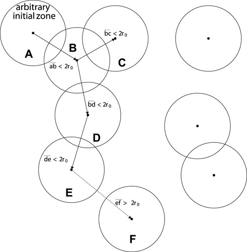
Figure 1. Illustration of Roach’s zone selection procedure. Zones (A–E) form a quintet, as the distance between any zone centers and at least one of the other zone centers in the spot is less than 2r₀. The distances between all zone centers in the spot and all zone centers not in the spot, beginning with (F), are greater than 2r₀. Figure adapted from [19].

The outcome of the neighbors overlapping test can be modeled with the binomial distribution. For instance, probability p₁ that the distance between a zone center and the center of the nearest neighboring zone is greater than 2r₀ (i.e., the first zone is a singlet) corresponds to the probability that no event occurs within a circular area of radius 2r₀ around the center of the first zone—let us call this coincidence area 4A₀, where A₀ is the area of an individual zone. Let us remember that the spatial distribution of the events is assumed to follow Poisson statistics. Introducing now our notation and defining k as the number of events falling within the coincidence area in a time frame Δt, the Poisson probability distribution for the number of events can be written as

$\mathrm{P}\mathrm{r}\left(k=i\right)=\frac{{\left(QE{n}_0\mathrm{\Delta }t4A_0\right)}^i{e}^{-QE{n}_0\mathrm{\Delta }t4A_0}}{i!},$

where QE is the quantum efficiency, defined as the ratio between the number of detected events and the total number of incoming events assuming no coincidence loss [21], which can be also expressed as

$QE=1-\mathrm{P}\mathrm{r}\left(\mathit{Mul}=0\right).(9)$

The introduction of QE arises from the fact that events that pass completely undetected do not contribute to the overall statistics (this statement is reviewed in Section 2.6). From these premises, it follows that p₁ can be written as

$p_1=\mathrm{P}\mathrm{r}\left(k=0\right)=e^{-QE{n}_0\mathrm{\Delta }t4A_0}.$

On the other hand, the probability that the distance between a zone center and the center of the nearest neighboring zone is less than 2r₀ is the complementary probability 1 − p₁. The chain of events that brings to an n-tet spot therefore consists of n − 1 sequences in which the nearest neighbor distances are less than 2r₀ and 1 sequence in which the nearest neighbor distance is greater, breaking the spot connection to the remaining zones. If the inter-zone distances are independent from each other—a condition that, as recognized by Roach, is approximately true and necessary to reduce the two-dimensional overlapping problem to a tractable form—the probability p_n for a zone to be part of an n-tet spot is the product of the individual probabilities:

$p_n=e^{-QE{n}_0\mathrm{\Delta }t4A_0}{\left(1-e^{-QE{n}_0\mathrm{\Delta }t4A_0}\right)}^{n-1}.$

Since each of the QEn₀Δt incoming events per unit area (corresponding to a pixel, in our case) per time frame has this probability of forming an n-tet spot, the number of zones contributing to the formation of n-tet spots is QEn₀Δt p_n. However, because n zones are required to form each spot, we need to weight by 1/n this value in order to obtain the expected number P_n of n-tet spots per unit area per time frame.

$P_n=QE{n}_0\mathrm{\Delta }t{p}_n/n,(10)$

$=QE{n}_0\mathrm{\Delta }t{e}^{-QE{n}_0\mathrm{\Delta }t4A_0}{\left(1-e^{-QE{n}_0\mathrm{\Delta }t4A_0}\right)}^{n-1}/n.$

The total number of spots $\mathcal{P}$ is the algebraic sum of all the n-tet spots, which converges analytically to

$\mathcal{P}={\displaystyle \sum _{n=1}^{\infty }}{P}_n,$

$=QE{n}_0\mathrm{\Delta }t\frac{QE{n}_0\mathrm{\Delta }t4A_0{e}^{-QE{n}_0\mathrm{\Delta }t4A_0}}{1-e^{-QE{n}_0\mathrm{\Delta }t4A_0}}.$

Defining now the random variable E(Δt) as the total number of recorded events per pixel in a time frame, its mean value coincides with p:

$\mathbb{E}\left[E\left(\mathrm{\Delta }t\right)\right]=\mathcal{P}.(11)$

The recorded event rate $e=\mathbb{E}\left[E(\mathrm{\Delta }t)\right]/\mathrm{\Delta }t$ can therefore be written as

$e={\left(QE{n}_0\right)}^2\mathrm{\Delta }t4A_0\frac{e^{-QE{n}_0\mathrm{\Delta }t4A_0}}{1-e^{-QE{n}_0\mathrm{\Delta }t4A_0}}.(12)$

At this point, it is suitable to bring to the attention to the reader that the Roach model was developed in a continuous two-dimensional domain and for the “simple” case of circular-shaped zones³, whereas our case involves a discretized domain (pixels) and random event shapes. Nevertheless, results shown in Section 3 suggest that the Roach model still provides an accurate description of the phenomenon, at the price of interpreting A₀ as a sort of effective quantity to be typically found via curve fitting, on the same line of what is done in [22] for the effective dead time in counting detectors with pulse shapes different from the ideal rectangular one. A rough a priori guess can anyway be attempted, imagining events to be more similar to squares rather than circles—a consequence of the pixelization of the space—with effective area $\mathbb{E}\left[\mathit{Mul}\right]$ and side $L=\sqrt{\mathbb{E}\left[\mathit{Mul}\right]}$. It is easy to find that this implies a correlation area equal to

$4A_0={\left(2L+1\right)}^2.(13)$

Let us now focus on the variance of the number of recorded events. Due to the complexity of the task in two dimensions, no model could be found neither by the author nor in the consulted literature. However, an analytical solution for the one-dimensional case exists and it deserves some attention. In the context of chromatography, an exact formulation based on statistical arguments was first achieved by Rowe and Davis [23] (see also [24] for a comprehensive summary of one-dimensional models):

$\mathbb{V}\left[P\left(\mathrm{\Delta }x\right)\right]=\lambda \mathrm{\Delta }x{e}^{-\lambda x_0}\left(1-2\lambda x_0{e}^{-\lambda x_0}\right),(14)$

where P corresponds to the number of recorded events in the one-dimensional space interval Δx, λ corresponds to the incoming event rate per unit space, and x₀ to the coincidence interval. Few years later, in the context of dead time models for paralyzable counting detectors, Yu and Fessler achieved independently and by analytical methods an equivalent formulation [25]—change Δx with the time interval t and x₀ with the system dead time τ. In their derivation, the term equivalent to $\lambda e^{-\lambda x_0}$ in Eq. 14 is explicitly identified with the recorded event rate p:

$p=\lambda e^{-\lambda x_0},(15)$

so that Eq. 14 could be rewritten as

$\mathbb{V}\left[P\left(\mathrm{\Delta }x\right)\right]=\mathrm{\Delta }xp\left(1-2x_{0}p\right).(16)$

By way of analogy, we propose to adapt this expression to the two-dimensional case by identifying p as the recorded event rate e of Eq. 12 integrated over the time frame Δt (in the one-dimensional context, indeed, rate is defined per unit spatial dimension), Δx as the number of pixels N_pix and x₀ as half the correlation area $\frac{4A_0}{2}$. This last relation is obtained by equivaleting the expressions for the recorded event rate in one and two dimensions for values of incoming event rates tending to zero, as reported in Appendix 4. Incidentally, it is worth noting that the one-dimensional expression is equivalent to the one for the singlets P₁ in two dimensions (see Eq. 10 with n = 1), which was, e.g., used to model, alone, the recorded event rate in two dimension in [21]. From the aforementioned proposition, it follows that the variance of the recorded events per pixel and in a time frame can be written as

$\mathbb{V}\left[E\left(\mathrm{\Delta }t\right)\right]=\mathrm{\Delta }te\left(1-4A_0\mathrm{\Delta }te\right),(17)$

$={\left(QE{n}_0\mathrm{\Delta }t\right)}^{2}4A_0\frac{e^{-QE{n}_0\mathrm{\Delta }t4A_0}}{1-e^{-QE{n}_0\mathrm{\Delta }t4A_0}}\left[1-{\left(QE{n}_0\mathrm{\Delta }t4A_0\right)}^2\frac{e^{-QE{n}_0\mathrm{\Delta }t4A_0}}{1-e^{-QE{n}_0\mathrm{\Delta }t4A_0}}\right].$

2.4 SNR and DQE₀

The knowledge of the first two momenta of the recorded statistics allows us to compute the corresponding SNR over a time frame, defined as

$SN{R}_{\mathcal{X}\left(\mathrm{\Delta }t\right)}=\frac{\mathbb{E}{\left[\mathcal{X}\left(\mathrm{\Delta }t\right)\right]}^2}{\mathbb{V}\left[\mathcal{X}\left(\mathrm{\Delta }t\right)\right]},$

which, thanks to the properties highlighted in Eqs 3, 4, can be easily generalized to the sum of a series of time frames:

$SN{R}_{\mathcal{X}\left(F_N\mathrm{\Delta }t\right)}=F_N\frac{\mathbb{E}{\left[\mathcal{X}\left(\mathrm{\Delta }t\right)\right]}^2}{\mathbb{V}\left[\mathcal{X}\left(\mathrm{\Delta }t\right)\right]}.$

More interesting, however, due to its importance and widespread use in the imaging community (see [26] and references therein for an interesting historical overview), is the DQE, defined as

$DQE=\frac{SN{R}_{\mathit{OUT}}}{SN{R}_{IN}},(18)$

where SNR_OUT is the signal-to-noise ratio referring to the recorded signal statistics and SNR_IN is the one referring to the incoming signal statistics, which, under the assumption of obeying Poisson statistics, equals to

$SN{R}_{IN\left(F_N\mathrm{\Delta }t\right)}=F_N{n}_0\mathrm{\Delta }t,(19)$

which makes the DQE independent on the number of acquired frames.

In its modern acceptance⁴, DQE is conceived in the two-dimensional domain of the spatial frequencies by applying Fourier transform to the output signal and noise. Use of frequency analysis requires the system to exhibit the properties of shift-invariance, linearity and wide-sense stationary statistics. In general, rarely, a system satisfies all the requirements in a rigorous manner. For example, a pixelated detector is not strictly shift-invariant, unless shifts are by an integer number of pixels. In addition, in a counting system, the noise is stationary only in conditions of uniform illumination as it depends on the incoming signal itself. Therefore, care must be taken when interpreting the results as they might be approximations of the true properties of the system [27, 28]. In our specific case, the requirement of linearity is clearly not satisfied. Since a straightforward extension of the theory is not well-established (see [29] for a nice compendium on possible generalizations of the concept of DQE to non-linear systems), we limit our analysis to the degenerate zero-frequency case denoted DQE₀⁵.

The DQE₀ of the recorded counts as a function of the incoming event rate can therefore be retrieved using Eqs 6, 8, 18, 19 in obtaining

$DQ{E}_{0_{\bar{M}}}=\frac{1-e^{-n_0\mathbb{E}\left[\mathit{Mul}\right]\mathrm{\Delta }t}}{n_0\mathrm{\Delta }t{e}^{-n_0\mathbb{E}\left[\mathit{Mul}\right]\mathrm{\Delta }t}\left[1+\left(\frac{\mathbb{E}\left[{\mathit{Mul}}^{\mathrm{2}}\right]}{\mathbb{E}\left[\mathit{Mul}\right]}-1\right)\frac{1-e^{-n_0\mathbb{E}\left[\mathit{Mul}\right]\mathrm{\Delta }t}}{n_0\mathbb{E}\left[\mathit{Mul}\right]\mathrm{\Delta }t}\right]},$

while one of the recorded events using Eqs 11, 17–19 obtaining

$DQ{E}_{0_E}=\frac{Q{E}^2{n}_0\mathrm{\Delta }t4A_0\frac{e^{-QE{n}_0\mathrm{\Delta }t4A_0}}{1-e^{-QE{n}_0\mathrm{\Delta }t4A_0}}}{1-{\left(QE{n}_0\mathrm{\Delta }t4A_0\right)}^2\frac{e^{-QE{n}_0\mathrm{\Delta }t4A_0}}{1-e^{-QE{n}_0\mathrm{\Delta }t4A_0}}}.$

2.5 Derived quantities

Additionally, derived quantities of particular interest, which we would like to mention, are the area occupancy (AO) and the coincidence loss fraction (CLF). The AO is defined as the ratio between the average number of counting pixels per frame and the total number of pixels, coinciding with the average number of recorded counts in a time frame.

$AO=\frac{N_{\mathit{pix}}\mathbb{E}\left[M\left(\mathrm{\Delta }t\right)\right]}{N_{\mathit{pix}}},$

$=\mathbb{E}\left[M\left(\mathrm{\Delta }t\right)\right].$

Information on the AO can have implications on the detector readout mechanism design and optimization, as well as on the choice of suitable data compression algorithms. The coincidence loss fraction is defined as the ratio between the number of “lost” events, i.e., not recorded, and the total number of incoming events.

$CLF=\frac{QE{n}_0-e}{QE{n}_0},(20)$

$=1-QE{n}_0\mathrm{\Delta }t4A_0\frac{e^{-QE{n}_0\mathrm{\Delta }t4A_0}}{1-e^{-QE{n}_0\mathrm{\Delta }t4A_0}}$

and reflects the counting efficiency of the system. In Eq. 20, the physical incoming event rate n₀ in the denominator is scaled by QE as QEn₀ is the actual ideal event rate recorded in the absence of coincidence loss.

2.6 General remarks

i. The study of the counting statistics of pixels featuring binary counts presented here complements a picture already including at least the classical paralyzable and non-paralyzable counting modes [25] and a particular case of the non-paralyzable mode [14], where the paralysis is avoided, thanks to a circuital stratagem called “instant retrigger.”

ii. The results on the recorded event statistics are of general validity, whether the hit digitization occurs directly in the pixel (with binary or non-binary outcome), in the readout electronics, or at the image processing stage. Differences can arise on the value of the coincidence area, according to the specific algorithm used for the event recognition.

iii. A detector with in-pixel counting electronics might have some advantages compared to one working in the charge integrating mode in terms of a slightly smaller coincidence area. It can indeed happen that a pixel receives, in the same time frame, signals originated by more than one event. If the front-end electronics works in the counting mode, the contribution of every event is individually processed (provided they do not undergo pile-up). If the front-end electronics works in the charge integrating mode, it is the sum of the contributions to be processed, making more probable the recording of a hit and the consequent formation of a “bridge” between neighboring events.

iv. The presented models were derived for systems with frame-based readout, but their validity can be extended to systems with the event-based readout as well. In a system with event-based readout, the detection of an event triggers its own readout, but the time stamp associated with it has finite resolution, and therefore, neighboring events within this time interval cannot be distinguished. The time-stamp discretization corresponds to our frame time⁶.

2.7 Monte Carlo simulation framework

To validate the analytical models, we used results of numerical simulations carried out with an improved version of the Monte Carlo tool used in [13, 30, 31]. The first step of the workflow was the creation of a statistically relevant pool of electron tracks in the semiconductor sensor. A total of 40 million tracks were generated using FLUKA⁷—a Monte Carlo particle transport and interaction suite [32, 33]—storing, for each of them, the three-dimensional spatial coordinates with an accuracy of 1 µm and the amount of energy released therein.

We then processed each individual electron track with a custom-developed numerical code mimicking the physics of the charge collection and signal formation at the pixelated electrode. The generated charge distribution of each track segment was thus propagated through the remaining sensor thickness to the pixels, and a Gaussian blurring was added to reproduce the effect of thermal diffusion, with a total width depending on an initial intrinsic contribution and, under the assumption of the constant electric field, to a contribution depending on the total travel length. The charge collected by each pixel was converted into energy and a counting threshold was applied, if the energy is higher, the pixel counts 1; otherwise, it counts 0. A random fluctuation representing the electronic noise, normally distributed and assumed uncorrelated among the pixels, was added to the signal. The response of both the sensor and the readout electronics has been assumed uniform in space. At this point, it was possible to extract the statistical distribution of the event multiplicity. Then, for each value of a series of incoming electron rates, a set of 2000 independent images (frames) was generated. The total number of impinging electrons for each individual frame was chosen randomly according to the suitable Poisson statistics and then they were uniformly and randomly distributed across the sensor surface, which covered an area of 2048 × 2048 pixels. A pixel cluster recognition algorithm was then applied to each frame to isolate single events. In order to be considered isolated, two clusters need to be separated by at least one empty pixel.

2.8 Case study

We chose a case study realistic for CryoEM applications consisting of a 25-µm-thick MAPS detector, covered with 5 µm of Al accounting for the metal layers and featuring square pixels of size 10 µm. The counting threshold energy was 1 keV, the electronic noise was 200 eV rms, and the thermal diffusion between 1 and 3 µm rms. The frame rate was assumed 1 kfps. The energy of the impinging electrons was 300 keV, with values of incoming rates in the range 1–200 el/s/pix.

3 Results and discussion

In order to get a visual feeling of the events distribution recorded on the pixel matrix, two frame sub-regions obtained with an incoming electron rate of 5 el/s/pix and 30 el/s/pix, respectively, are shown in Figure 2. The first can be considered an example of low incoming rate condition, the second an example of medium incoming rate condition, with event clumping clearly noticeable.

Figure 2

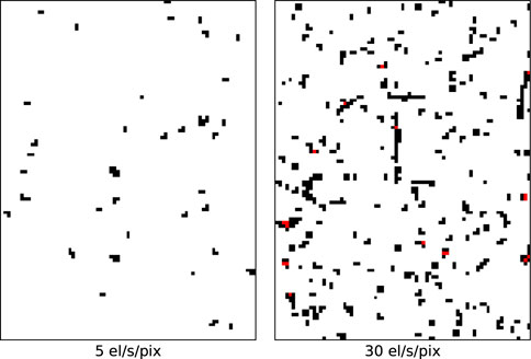
Figure 2. Example of frames sub-regions obtained with an incoming electron flux of 5 el/s/pix (left) and 30 el/s/pix (right). Pixels with overlapping events have been highlighted in red for visualization purposes.

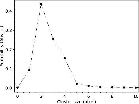
The single-event multiplicity probability distribution, computed in a condition of no coincidence loss, is shown in Figure 3. The large majority of clusters consist of 1–4 pixels, with a peak of probability at 2. Cluster sizes greater than 4 exist with lower occurrence probability. In addition, the case of no detection, i.e., cluster size 0, is very unlikely with probability 0.002. This allows us to infer the quantum efficiency through Eq. 9, yielding QE = 0.998. The first two statistical momenta of the distribution, fundamental for the continuation, are $\mathbb{E}\left[\mathit{Mul}\right]=2.87$ pix and $\mathbb{E}\left[{\mathit{Mul}}^2\right]=12.93$ pix².

Figure 3

Figure 3. Single-event multiplicity probability distribution. Lines are to guide the eye.

Figure 4 (top) shows the comparison between recorded count rate curves obtained with numerical simulations and predicted by the analytical model of Eq. 7, as a function of the incoming electron rate. The ideal count rate curve $n_0\mathbb{E}\left[\mathit{Mul}\right]$ is also shown as reference. Figure 4 (bottom) shows the corresponding error in percentage, which is on the order of few per mill across all the range of probed incoming electron rates. In addition, as a quantitative measure of the goodness-of-fit, we computed the L² relative error norm (L²REN), defined as

$L^{2}REN\left(x\right)=\sqrt{\frac{{\sum }_{i=1}^{\mathit{NoP}}{\left(x_i^{\mathit{sim}}-x_i^{\mathit{ana}}\right)}^2}{{\sum }_{i=1}^{\mathit{NoP}}{\left(x_i^{\mathit{ana}}\right)}^2}},$

where NoP corresponds to the number of simulated points. In this case, it amounts to 0.13%.

Figure 4

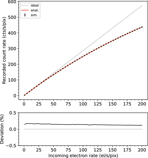
Figure 4. (Top) Comparison between recorded count rate curves obtained with numerical simulations (error bars) and predicted by the analytical model of Eq. 7 (solid line). Please note that the error bars on the simulated values are smaller than the graphical symbol. The ideal count rate curve is also shown as reference. (Bottom) Deviation expressed in percentage.

Figure 5 (top) shows the comparison between recorded count variances in one time frame obtained with the numerical simulations and predicted by the analytical model of Eq. 8, as a function of the incoming electron rate. The Poisson variance values of the incoming electron statistics n₀Δt and of the ideal recorded counts $n_0\mathbb{E}\left[{\mathit{Mul}}^{\mathrm{2}}\right]\mathrm{\Delta }t$ [14] are also shown as reference. Figure 5 (bottom) shows the corresponding error in percentage. The L²REN amounts to 3.97%.

Figure 5

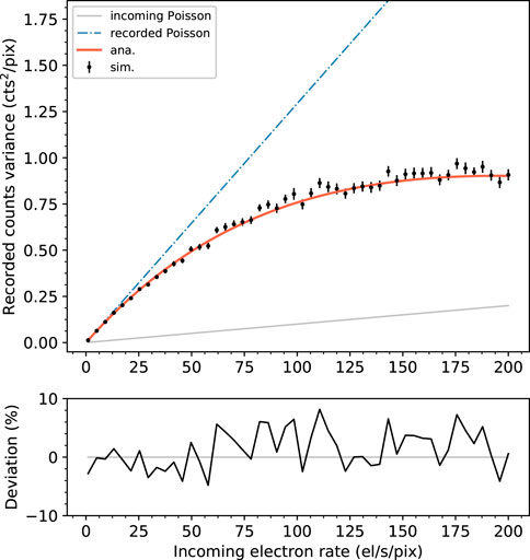
Figure 5. (Top) Comparison between recorded count variances in one time frame obtained with the numerical simulations (error bar) and predicted by the analytical model of Eq. 8 (solid line). The Poisson variance of the incoming electron statistics and of the ideal recorded counts is also shown as reference. (Bottom) Deviation between the two curves expressed in percentage.

The level of agreement between simulated and predicted data for both for the mean and the variance is such that we can positively conclude on the validity of the proposed model.

Figure 6 (top) shows the comparison between recorded electron rate curves simulated and fitted with the analytical models, as a function of the incoming electron rate. We first observe that the counting paralysis occurs here much earlier than for the bare counts in Figure 4, due to the inflating effect of the event multiplicity. Then, the curve labeled “ana. 2D” corresponds to the result using the Roach model of Eq. 12, whose fitting yields a value of 4A₀ = 20.51 pixels. For accuracy reasons, the fitting was restricted to a range of incoming electron rate 0–80 el/s/pix (the upper bound corresponds to the location of the maximum recorded electron rate) as above this limit, the model tends to overestimate the number of recorded electrons. Within this range, the L²REN of the Roach model amounts to 0.06%. Incidentally, we note that using the Roach model of Eq. 13 to estimate a priori the correlation area 4A₀, we obtain a value of 19.26, which is not far from the correct value obtained through the fitting. The curves labeled with “ana. P_n” show the breakdown of the Roach model into the first five n-tet spot components, namely, the singlet, doublet, tripled, quartet, and quintet spots, computed with Eq. 10. It is interesting to note how the contribution of lower-order n-tet spots is always dominant on higher-order spots over all the range of incoming electron rates. To some extent, this explains why the one-dimensional model of Eq. 15 (mathematically equivalent to the number of singlets in the two-dimensional model) with parameter $x_0=\frac{4A_0}{2}=10.255$, labeled in Figure 6 as “ana. 1D,” also provides an acceptable approximation of the simulated data, in particular at low values of incoming electron rates. This statement is supported also by Figure 6 (bottom), which shows the corresponding fitting errors in percentage.

Figure 6

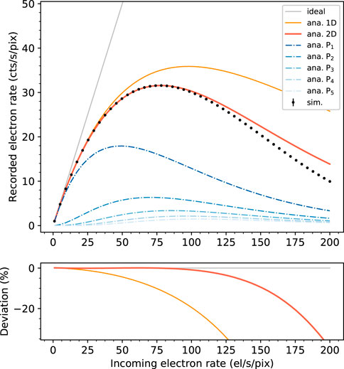
Figure 6. (Top) Recorded electron rate curves obtained with the numerical simulations (error bars) and their fitting with the analytical models (solid lines). “ana. 2D” corresponds to the fitting with the Roach model of Eq. 12, while “ana. P_n” corresponds to the contributions of the n-tet spots up to n = 5 using Eq. 10. “ana. 1D” corresponds to the fitting with the one-dimensional model of Eq. 15. Please note that the error bars on the simulated valued are smaller than the graphical symbol. The ideal recorded electron rate curve n₀ is also shown as the reference. (Bottom) Deviation between the numerical simulations and their fitting with analytical models expressed in percentage.

Figure 7 (top) shows the recorded electrons variance in one time frame, as a function of the incoming electron rate. The curve labeled “ana. 1D,” corresponds to the one-dimensional analytical solution in Eq. 16, while the curve labeled “proposed ana. 2D” corresponds to the proposed extension of the one-dimensional model to the two-dimensional case, as in Eq. 17. The Poisson variance of the incoming electrons statistics n₀Δt is also shown as the reference. We observe that up to the incoming electron rate of ∼30 el/s/pix (corresponding to a coincidence loss of 27.6%, see Figure 9), both models describe the behavior of the recorded variance equally well, with a L²REN of 6.8%. For increasing incoming electron rates, both models underestimate the data down to a factor 1/2, as shown in Figure 7 (bottom). The proposed model, however, follows the peculiar “bulged” shape of the simulation better than the original one-dimensional one. For this reason and because it also leads to a simpler expression of the DQE0E, we endorse the adoption of the proposed model for the two-dimensional case.

Figure 7

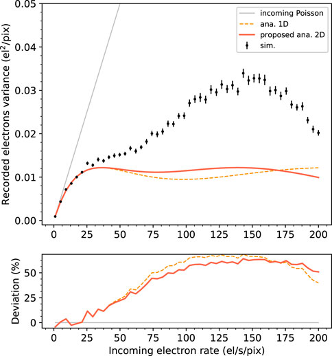
Figure 7. (Top) Recorded count variance obtained with the numerical simulations (error bars) and predicted with the analytical models (solid lines). “ana. 1D” corresponds to the result obtained with the one-dimensional model of Eq. 16, while “proposed ana. 2D” corresponds to the result obtained with our proposed two-dimensional extension of Eq. 17. As reference, the Poisson variance of the incoming electrons is also shown. (Bottom) Deviation between the two curves expressed in percentage.

The behavior of the DQE₀ as a function of the incoming electron rate is reported in Figure 8, for both the cases of recorded counts and recorded electrons. The knowledge of the first two statistical momenta of the multiplicity distribution allows us to compute the limiting value of the DQE_0M for low incoming electron rates⁸:

$\underset{n_0\to 0}{\lim }DQ{E}_{0_{\bar{M}}}=\frac{\mathbb{E}{\left[\mathit{Mul}\right]}^2}{\mathbb{E}\left[{\mathit{Mul}}^2\right]},$

which, in our case, amounts to 0.64. For the DQE_0E, on the other hand, it holds

$\underset{n_0\to 0}{\lim }DQ{E}_{0_E}=QE,$

which, in our case, is 0.998. For increasing incoming electron rates, DQE_0E shows a non-monotonic behavior, while DQE_0M grows indefinitely. We can attempt to explain the increasing trend for both DQE_0M and DQE_0E—for the latter before the unavoidable collapse at high incoming rates due to counting paralysis—in an analogous way of what is already observed in [14] in the time domain. Essentially, but probably less intuitively, event overlapping provides a sort of “regularizing” effect of the recorded statistics. For instance, a recorded event resulting from the union of several overlapping events is recorded, regardless (to some extent) of the variation in number and position of the single events constituting the union, making it less sensitive to the natural statistical fluctuations of the incoming signal, in a sort of noise filtering effect. However, one should not be tempted to think that operating a detector in this regime would be absolutely beneficial. Indeed, the gain in DQE₀ is compensated by a loss in spatial resolving capability due to the increasing size of the merged event.

Figure 8

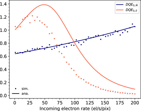
Figure 8. Simulated (symbols) and analytically modeled (solid lines) DQE₀ for the recorded counts and for the recorded electrons.

Finally, Figure 9 shows the area occupancy and the coincidence loss fraction as a function of the incoming electron rate. In the context of cryoEM applications, only tiny deviations from linearity are acceptable—on the order of few percent. Assuming a relaxed upper limit for the coincidence loss fraction of 10% [21], this is reached in our case study for an incoming electron rate of 10.10 el/s/pix and the corresponding area occupancy is 2.86%. In this regime, it is, therefore, perfectly justified the use of both the Roach model for the recorded electron rate and of the proposed two-dimensional model for the recorded electron variance. To give a more practical understanding of the impact of distortions of counting statistics, it is useful to translate the aforementioned quantities into integrated values over the detector area (2048 × 2048 pixels) and frame time (1 ms). A coincidence loss fraction of 10% would then occur at an incoming electron count of 41'943 el, for a corresponding AO of 119'957 pix.

Figure 9

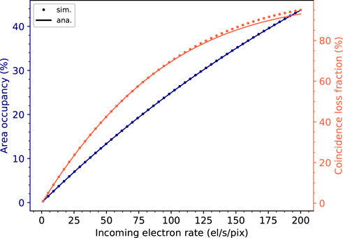
Figure 9. Simulated (symbols) and analytically modeled (solid lines) area occupancy and coincidence loss fraction.

4 Conclusion

We investigated the impact of coincidence loss on the recorded count statistics and on the noise performance in counting detectors featuring sparse binary images. First, we derived exact analytical expressions for the mean and the variance of the recorded counts. Second, we addressed the problem of the mean and variance of the recorded events (i.e., pixel clusters identified as a single incoming event). We reviewed, reinterpreted, and evaluated the suitability of approximated models—as no exact solutions exist in two dimensions—previously obtained in several different disciplines, adopting the “Roach model” for the mean and proposing an extension of the one-dimensional exact solution for the variance to the two-dimensional case. For both cases, we derived expressions for the SNR and the DQE₀. Model predictions were qualified against numerical simulation carried out with a custom-developed Monte Carlo code, for the CryoEM-realistic case study of a 25-µm-thick MAPS detector featuring a pixel size of 10 μm, a frame rate of 1 kfps, and working in the binary counting mode. The incoming beam consisted of electrons with energy 300 keV and with flux intensities up to 200 el/s/pix, where coincidence loss phenomena are bringing the system well into paralysis. The matching between simulated data and analytical prediction is perfect for the mean and variance of the recorded counts. For the mean recorded electrons, the Roach model fits excellently simulated data up to an incoming electron rate of ∼80 el/s/pix, corresponding to the location of the maximum of the recorded curve. At higher values of incoming rates, the model tends to slightly overestimate the number of recorded events. For the variance of the recorded events, both the existing one-dimensional and the proposed two-dimensional analytical solutions match the simulated data excellently up to an incoming electron rate of ∼30 el/s/pix. At higher values of incoming rates, both models severely underestimate the data, but the proposed two-dimensional extension follows better functional behavior, supporting its adoption. The resulting DQE₀ shows an increasing behavior as a function of the incoming rate for the recorded counts, while it shows a non-monotonic behavior for the recorded events. The increase above the low incoming rate limit is due to an allegedly reduced sensitivity of the recorded signals resulting from the union of multiple events to the statistical fluctuations of the individual incoming events, in a sort of noise filtering effect. Only in the second case, it ultimately decreases to zero due to the overwhelming system paralysis. Generalization and limitations to the validity of the models were also discussed.

Data availability statement

The raw data supporting the conclusion of this article will be made available by the authors, without undue reservation.

Author contributions

PZ: writing–original draft and writing–review and editing.

Funding

The author(s) declare that no financial support was received for the research, authorship, and/or publication of this article.

Acknowledgments

The author would like to thank J. M. Davis for the kind conversation.

Conflict of interest

Author PZ was employed by DECTRIS Ltd.

Publisher’s note

All claims expressed in this article are solely those of the authors and do not necessarily represent those of their affiliated organizations, or those of the publisher, the editors, and the reviewers. Any product that may be evaluated in this article, or claim that may be made by its manufacturer, is not guaranteed or endorsed by the publisher.

Footnotes

¹In the classical paralyzable counting mode, each incoming event paralyzes the system for another dead time period, leading to the relation between the incoming rate n and the recorded rate m:

$m=n{e}^{-n\tau }(1)$

where τ corresponds to the system dead time.In the classical non-paralyzable counting mode, on the other hand, only the first detected event of a series paralyzes the system for a single dead time period, leading to the relation:

$m=\frac{n}{1+n\tau }.(2)$

²For example, by analyzing the statistical distribution of the cluster sizes generate by single, non-overlapping incoming events. Please note that the knowledge of the real incoming flux is needed since $\mathit{Mul}$ includes events with size 0, which are by definition not detected.

³Considerations on the case of elliptical zones are, however, reported in [18, 20].

⁴Originally, the DQE was conceived as a “large area” property, what is nowadays called zero-frequency DQE [26].

⁵The notation DQE₀ is preferred over DQE(0) not to induce to think that the DQE is an actual function of frequency.

⁶Modern event-based readout chips can feature time-stamp discretization down to ns or sub-ns levels, allowing in line of principle for count rate capabilities orders of magnitude better than frame-based ones. A practical limit anyway arises from the fact that transmitting spatial coordinates and timing information to the readout electronics potentially generates huge amount of data, saturating the system bandwidth. Although much depends on the specific implementation details, the advantage of one readout mode over the other is not obvious.

⁷v. 4-2.1. The physics was set to multiple Coulomb scattering with the cutoff energy of 1 keV for electrons and 100 eV for photons. Fluorescence was enabled, and no biasing was used.

⁸A result of general validity for counting detectors [34].

References

1. Müller JW. Dead-time problems. Methods Phys Res (1973) 112:47–57. doi:10.1016/0029-554X(73)90773-8

CrossRef Full Text | Google Scholar

2. Knoll GF. Radiation detection and measurement. 3rd ed. John Wiley & Sons, Inc. (2000). p. 119–22. Chapter 3.

Google Scholar

3. Renaud J-P, Chari A, Ciferri C, Liu W-t., Rémigy H-W, Stark H, et al. Cryo-EM in drug discovery: achievements, limitations and prospects. Nat Rev Drug Discov (2018) 17:471–92. doi:10.1038/nrd.2018.77

PubMed Abstract | CrossRef Full Text | Google Scholar

4. Peet MJ, Henderson R, Russo CJ. The energy dependence of contrast and damage in electron cryomicroscopy of biological molecules. Ultramicroscopy (2019) 203:125–31. doi:10.1016/j.ultramic.2019.02.007

PubMed Abstract | CrossRef Full Text | Google Scholar

5. Deptuch G, Besson A, Rehak P, Szelezniak M, Wall J, Winter M, et al. Direct electron imaging in electron microscopy with monolithic active pixel sensors. Ultramicroscopy (2007) 107(8):674–84. doi:10.1016/j.ultramic.2007.01.003

PubMed Abstract | CrossRef Full Text | Google Scholar

6. Guerrini N, Turchetta R, Van Hoften G, Henderson R, McMullan G, Faruqi AR A high frame rate, 16 million pixels, radiation hard CMOS sensor. J Instrumentation (2011) 6(03):C03003. doi:10.1088/1748-0221/6/03/C03003

CrossRef Full Text | Google Scholar

7. Li X, Mooney P, Zheng S, Booth CR, Braunfeld MB, Gubbens S, et al. Electron counting and beam-induced motion correction enable near-atomic-resolution single-particle cryo-EM. Nat Methods (2013) 10:584–90. doi:10.1038/nmeth.2472

PubMed Abstract | CrossRef Full Text | Google Scholar

8. McMullan G, Faruqi AR, Clare D, Henderson R. Comparison of optimal performance at 300keV of three direct electron detectors for use in low dose electron microscopy. Ultramicroscopy (2014) 147:156–63. doi:10.1016/j.ultramic.2014.08.002

PubMed Abstract | CrossRef Full Text | Google Scholar

9. Naydenova K, McMullan G, Peet MJ, Lee Y, Edwards PC, Chen S, et al. CryoEM at 100 keV: a demonstration and prospects. IUCrJ (2019) 6:1086–98. doi:10.1107/s2052252519012612

PubMed Abstract | CrossRef Full Text | Google Scholar

10. McMullan G, Naydenova K, Mihaylov D, Yamashita K, Peet MJ, Wilson H, et al. Structure determination by cryoEM at 100 keV. PNAS (2023) 120(49):e2312905120. doi:10.1073/pnas.2312905120

PubMed Abstract | CrossRef Full Text | Google Scholar

11. McMullan G, Clark AT, Turchetta R, Faruqi AR. Enhanced imaging in low dose electron microscopy using electron counting. Ultramicroscopy (2009) 109:1411–6. doi:10.1016/j.ultramic.2009.07.004

PubMed Abstract | CrossRef Full Text | Google Scholar

12. McMullan G, Turchetta R, Faruqi AR. Single event imaging for electron microscopy using MAPS detectors. J Instrum (2011) 6:C04001. doi:10.1088/1748-0221/6/04/c04001

CrossRef Full Text | Google Scholar

13. Zambon P. Enhanced DQE and subpixel resolution by single-event processing in counting hybrid pixel electron detectors: a simulation study. Front Phys (2023) 11:1123787. doi:10.3389/fphy.2023.1123787

CrossRef Full Text | Google Scholar

14. Zambon P. Temporal and spatial variance in pixelated counting detectors with dead time and retrigger capability. Nucl Inst. Methods Phys Res A (2022) 1032:166625. doi:10.1016/j.nima.2022.166625

CrossRef Full Text | Google Scholar

15. Roach SA. The theory of random clumping. London: Methuen (1968).

Google Scholar

16. Aldous D. Probability approximations via the Poisson clumping heuristic. Appl Math Sci (1989) 7. doi:10.1007/978-1-4757-6283-9

CrossRef Full Text | Google Scholar

17. Davis JM, Giddings JC. Statistical theory of component overlap in multicomponent chromatograms. Anal Chem (1983) 55:418–24. doi:10.1021/ac00254a003

CrossRef Full Text | Google Scholar

18. Davis JM. Statistical theory of spot overlap in two-dimensional separations. Anal Chem (1991) 63:2141–52. doi:10.1021/ac00019a014

CrossRef Full Text | Google Scholar

19. Oros FJ, Davis JM. Comparison of statistical theories of spot overlap in two-dimensional separations and verification of means for estimating the number of zones. J Chromatogr (1992) 591:1–18. doi:10.1016/0021-9673(92)80218-j

CrossRef Full Text | Google Scholar

20. Davis JM. Statistical theory of spot overlap for n-dimensional separations. Anal Chem (1993) 65:2014–23. doi:10.1021/ac00063a015

CrossRef Full Text | Google Scholar

21. Li X, Zheng SQ, Egami K, Agard DA, Cheng Y Influence of electron dose rate on electron counting images recorded with the K2 camera. J Struct Biol (2013) 184:251–60. doi:10.1016/j.jsb.2013.08.005

PubMed Abstract | CrossRef Full Text | Google Scholar

22. Zambon P. Dead time model for X-ray photon counting detectors with retrigger capability. Nucl Inst. Methods Phys Res A (2021) 994:165087. doi:10.1016/j.nima.2021.165087

CrossRef Full Text | Google Scholar

23. Rowe K, Davis JM Error analysis of parameters determined with statistical models of overlap from nonhomogeneous separations. Chemometrics Intell Lab Syst (1997) 28:109–26. doi:10.1016/s0169-7439(97)00053-1

CrossRef Full Text | Google Scholar

24. Felinger A. Chapter 15: statistical theory of peak overlap, data analysis and signal processing in chromatography. Elsevier (1998).

Google Scholar

25. Yu DF, Fessler JA. Mean and variance of single photon counting with deadtime. Phys Med Biol (2000) 45:2043–56. doi:10.1088/0031-9155/45/7/324

PubMed Abstract | CrossRef Full Text | Google Scholar

26. Ji X, Feng M, Zhang R, Chen G-H, Li K. An experimental method to directly measure DQE$(k)$ at k  =  0 for 2D x-ray imaging systems. Physmed Biol (2019) 64(7):075013. doi:10.1088/1361-6560/ab10a2

PubMed Abstract | CrossRef Full Text | Google Scholar

27. Williams MB, Mangiafico PA, Simoni PU. Noise power spectra of images from digital mammography detectors. Med Phys (1999) 26:1279–93. doi:10.1118/1.598623

PubMed Abstract | CrossRef Full Text | Google Scholar

28. Friedman SN, Fung GSK, Siewerdsen JH, Tsui BMW. A simple approach to measure computed tomography (CT) modulation transfer function (MTF) and noise-power spectrum (NPS) using the American College of Radiology (ACR) accreditation phantom. Med Phys (2013) 40(5):051907. doi:10.1118/1.4800795

PubMed Abstract | CrossRef Full Text | Google Scholar

29. McDonald MC. A method to measure the detective quantum efficiency of radiographic systems in clinical setting, electronic thesis and dissertation repository (2012). p. 484.

Google Scholar

30. Fernandez-Perez S, Boccone V, Broennimann C, Disch C, Piazza L, Radicci V, et al. Characterization of a hybrid pixel counting detector using a silicon sensor and the IBEX readout ASIC for electron detection. In: Jinst 16 P10034 (2021). doi:10.1088/1748-0221/16/10/P10034

CrossRef Full Text | Google Scholar

31. Zambon P, Bottinelli S, Schnyder R, Musarra D, Boye D, Dudina A, et al. KITE: high frame rate, high count rate pixelated electron counting ASIC for 4D STEM applications featuring high-Z sensor. Nucl Inst. Methods Phys Res A (2023) 1048:167888. doi:10.1016/j.nima.2022.167888

CrossRef Full Text | Google Scholar

32. Ferrari A, Sala PR, Fasso A, Ranft J. Fluka: a multi-particle transport code (2005). Program version (2005). [INFN-TC-05-11]. doi:10.5170/CERN-2005-010

CrossRef Full Text | Google Scholar

33. Böhlen T, Cerutti F, ChinM FA, Ferrari A, Ortega P, et al. The FLUKA code: developments and challenges for high energy and medical applications. Nucl Data Sheets (2014) 120:211–4. doi:10.1016/j.nds.2014.07.049

CrossRef Full Text | Google Scholar

34. McMullan G, Cattermole DM, Chen S, Henderson R, Llopart X, Summerfield C, et al. Electron imaging with Medipix2 hybrid pixel detector. Ultramicroscopy (2007) 107:401–13. doi:10.1016/j.ultramic.2006.10.005

PubMed Abstract | CrossRef Full Text | Google Scholar

Appendix A: Derivation of the relation between x₀ and A₀

In one spatial dimension the recorded event rate per unit length and unit time p can be expressed as:

$p\left(\lambda \right)=\lambda e^{-\lambda \mathrm{\Delta }t{x}_0}(\mathrm{A1})$

where λ represents the incoming event rate per unit length and unit time which in our case is λ = QEn₀. The term Δt does not appear in Eq. 14 as it is implicit in the incoming rate definition which is expressed per unit length. In two spatial dimensions, the recorded event rate per unit area and unit time e is, from Eq. 12:

$e\left(\lambda \right)={\lambda }^2\mathrm{\Delta }t4A_0\frac{e^{-\lambda \mathrm{\Delta }t4A_0}}{1-e^{-\lambda \mathrm{\Delta }t4A_0}}.(\mathrm{A2})$

The goal is to find the value of x₀ as a function of A₀ such that p ∼ e for λ → 0. As initial step, however, we note that to simplify the computation both p and e can be divided by λ, so let us defined the normalized quantities $\widehat{p}=p/\lambda$ and $\widehat{e}=e/\lambda$. Then, we express them with their Maclaurin series up to first degree, which gives:

$\widehat{p}\left(\lambda \right)\sim \widehat{p}\left(0\right)+{\widehat{p}}^{\prime }\left(0\right)\lambda (\mathrm{A3})$

$\widehat{e}\left(\lambda \right)\sim \widehat{e}\left(0\right)+{\widehat{e}}^{\prime }\left(0\right)\lambda (\mathrm{A4})$

where the apex ′ denotes the derivative of the function with respect to λ.

For $\widehat{p}$ it holds $\widehat{p}(0)=1$ and ${\widehat{p}}^{\prime }(0)=-\mathrm{\Delta }t{x}_0$.

For $\widehat{e}$, on the other hand, $\underset{\lambda \to 0}{\lim }\widehat{e}(\lambda )$ gives the indefinite form $\frac{0}{0}$. Using L’Hôpital’s rule we get:

$\underset{\lambda \to 0}{\lim }\widehat{e}\left(\lambda \right)=\frac{\mathrm{\Delta }t4A_0{e}^{-\lambda \mathrm{\Delta }t4A_0}\left(1-e^{-\lambda \mathrm{\Delta }t4A_0}\right)}{\mathrm{\Delta }t4A_0{e}^{-\lambda \mathrm{\Delta }t4A_0}}=1.(\mathrm{A5})$

Also for ${\widehat{e}}^{\prime }$, which is:

${\widehat{e}}^{\prime }=-\frac{\mathrm{\Delta }t4A_0\left[\left(\lambda \mathrm{\Delta }t4A_0-1\right)e^{\lambda \mathrm{\Delta }t4A_0}+1\right]}{{\left(e^{\lambda \mathrm{\Delta }t4A_0}-1\right)}^2}(\mathrm{A6})$

the $\underset{\lambda \to 0}{\lim }{\widehat{e}}^{\prime }(\lambda )$ leads to the $\frac{0}{0}$ indefinite form, which can be solved using twice L’Hôpital’s rule:

$\underset{\lambda \to 0}{\lim }{\widehat{e}}^{\prime }\left(\lambda \right)=-\frac{{\left(\mathrm{\Delta }t4A_0\right)}^3\left(\lambda \mathrm{\Delta }t4A_0+1\right)e^{\lambda \mathrm{\Delta }t4A_0}}{2{\left(\mathrm{\Delta }t4A_0\right)}^2{e}^{\lambda \mathrm{\Delta }t4A_0}\left(2e^{\lambda \mathrm{\Delta }t4A_0}-1\right)}=-\frac{\mathrm{\Delta }t4A_0}{2}.(\mathrm{A7})$

Eqs A3, A9 therefore become:

$\widehat{p}\left(\lambda \right)\sim 1-\mathrm{\Delta }t{x}_0\lambda (\mathrm{A8})$

$\widehat{e}\left(\lambda \right)\sim 1-\frac{\mathrm{\Delta }t4A_0}{2}\lambda (\mathrm{A9})$

and equaling the terms it is straightforward to see that $x_0=\frac{4A_0}{2}$.