Stochastic modeling of plant-insect interaction dynamics with MEMS-based monitoring and noise effects

The dynamics of plant-insect interactions play a crucial role in the ecosystem, influenced by complex molecular signaling pathways. This study extends existing deterministic models of plant-insect systems by incorporating stochastic elements and molecular interactions, particularly focusing on the roles of Botrytis Induced Kinase-1 (BIK1) and Phyto Alexin Deficient-4 (PAD4) proteins. The model evaluates the effects of constant inhibition, pulsed inhibition, and adaptive feedback control on plant biomass $(y_1)$, insect herbivore density $(y_2)$, PAD4 levels $(y_3)$, and BIK1 levels $(y_4)$. Additionally, we examine the impact of different noise types, including deterministic, Gaussian, and Lévy noise, on system variability and stability. Results indicate that our stochastic model is superior as it shows a significant reduction in BIK1 levels, particularly under higher noise intensities, which enhances PAD4 activity and improves plant defense mechanisms. Moreover, moderate noise intensity $(\sigma =0.05)$ provides an optimal balance, sustaining PAD4 levels while effectively controlling insect herbivore populations. We also integrate MEMS-based feedback mechanisms, which dynamically adjust plant biomass and molecular signaling, further stabilizing the system’s response to environmental variability.

1 Introduction

The intricate dynamics of plant-insect interactions have long captivated ecologists and biologists due to their profound implications for ecosystem stability and agricultural productivity. A notable example of such interaction is the relationship between plants and herbivorous insects, such as aphids, which are significant contributors to crop damage and yield loss globally [1]. Plants have evolved sophisticated defense mechanisms to counteract these insect attacks, initiating a complex interplay of molecular signals and physiological responses aimed at mitigating damage and ensuring survival [2, 3]. In this context, the role of Botrytis Induced Kinase-1 $(BIK1)$ has emerged as a critical component of the plant defense arsenal. BIK1 is involved in the phosphorylation of the flagellin receptor FLS2 and BAK1 proteins, initiating a cascade of defense responses that include the production of phytoalexins and other defensive compounds [4]. These responses are modulated by signaling pathways mediated by jasmonic acid (JA) and salicylic acid (SA), which are crucial for the activation of plant immune responses [5, 6]. Recent research has highlighted the interaction between BIK1 and Phytoalexin Deficient-4 (PAD4), another key player in the plant defense response. PAD4 is known to enhance the plant’s resistance to aphids by promoting the synthesis of antixenotic compounds that deter insect feeding [7]. However, $BIK1$ has been shown to suppress PAD4 expression, thereby modulating the plant’s defensive capabilities [8]. Given the pivotal roles of $BIK1$ and $PAD4$ in plant-insect interactions, understanding the molecular underpinnings of their interaction and its impact on plant health is of paramount importance. We further enhance the deterministic model [9] by incorporating MEMS-based feedback mechanisms, allowing for real-time dynamic adjustments in plant biomass and molecular signaling based on environmental conditions and sensor data. Our study addresses critical gaps in existing research by incorporating stochastic elements to capture the inherent variability and extreme events in these systems, offering novel insights into how molecular signaling pathways influence plant defense mechanisms and herbivore population dynamics. The model simulates the dynamics of plant biomass (P), insect herbivore density (I), $PAD4$ protein, and $BIK1$ protein under various conditions. Mathematical modeling has evolved from deterministic approaches, such as those by [10, 11], to stochastic models that account for variability and randomness, as highlighted by [12, 13], and [14]. These stochastic models provide a more realistic depiction of ecological systems by incorporating environmental noise, as seen in works like [15, 16].

The stochastic processes, particularly Lévy noise, enhances the model’s ability to capture extreme events, such as insect outbreaks, which are not well represented by Gaussian noise alone. Stochastic modeling techniques, as demonstrated by [17, 18], offer valuable insights for predicting population dynamics, evaluating control strategies, and understanding the influence of environmental variability. The use of Lévy noise in our model allows for the simulation of significant, abrupt changes in plant-insect interactions, providing a comprehensive representation of random phenomena. This approach underscores the importance of stochastic models in understanding complex biological systems and informing agricultural and environmental management practices. The characteristic function of a Lévy process is given by,

$\mathbb{E}\left[e^{iuL\left(t\right)}\right]=\exp \left(t\left(iu\gamma -\frac{1}{2}{\sigma }^2{u}^2+{\int }_{\mathbb{R}\backslash \left\{0\right\}}\left(e^{iux}-1-iux{\mathbf{1}}_{|x|<1}\right)\nu \left(dx\right)\right)\right),$

where $\gamma$ represents the drift coefficient, ${\sigma }^2$ is the variance of the Gaussian part, and $\nu$ is the Lévy measure that describes the jump intensity and distribution.

The plant-insect interaction system is a well-studied model in ecology, evolving from predator-prey analogies to more sophisticated mathematical models incorporating plant immunity concepts. This study extends these models by including molecular interactions in the plant defense system, inspired by [9]. The primary objective of this research is to develop a stochastic mathematical model to analyze plant-insect interaction dynamics, focusing on the molecular interplay between $PAD4$ and $BIK1$ proteins. It explores the impact of noise types, deterministic, Gaussian, and Lévy noise on the system’s variability and stability. This research contributes to understanding plant-insect interactions at the molecular level, with potential applications in agriculture. It highlights the benefits of adaptive feedback control for plant protection, dynamically adjusting to changing conditions. By incorporating noise, especially Lévy noise, the model captures extreme fluctuations, providing a realistic depiction of variability in plant-insect interactions. The study aims to answer key questions about the effects of control strategies, noise types, and the broader ecological implications of these findings.

2 Model equations

The system of differential equations governing the deterministic model is [9],

$\begin{array}{cc}\hfill \frac{d{y}_1}{dt}& =a_1{y}_1\left(1-\frac{y_1}{K}\right)-a_2{y}_1{y}_2,\hfill \\ \hfill \frac{d{y}_2}{dt}& =a_3{y}_1{y}_2-a_4{y}_2-a_5{y}_3{y}_2,\hfill \\ \hfill \frac{d{y}_3}{dt}& =a_6{y}_1{y}_2-a_7{y}_3-a_8{y}_3{y}_4,\hfill \\ \hfill \frac{d{y}_4}{dt}& =a_9{y}_1{y}_2-a_{10}{y}_4-a_{11}\cdot I{n}_{\mathit{BIK1}}.\hfill \end{array}(1)$

The stochastic differential equations is,

$\begin{array}{cc}\hfill d{y}_1& =\left(a_1{y}_1\left(1-\frac{y_1}{K}\right)-a_2{y}_1{y}_2\right)dt+{\sigma }_1{y}_{1}d{W}_1,\hfill \\ \hfill d{y}_2& =\left(a_3{y}_1{y}_2-a_4{y}_2-a_5{y}_3{y}_2\right)dt+{\sigma }_2{y}_{2}d{W}_2,\hfill \\ \hfill d{y}_3& =\left(a_6{y}_1{y}_2-a_7{y}_3-a_8{y}_3{y}_4\right)dt+{\sigma }_3{y}_{3}d{W}_3,\hfill \\ \hfill d{y}_4& =\left(a_9{y}_1{y}_2-a_{10}{y}_4-a_{11}\cdot I{n}_{\mathit{BIK1}}\right)dt+{\sigma }_4{y}_{4}d{W}_4,\hfill \end{array}(2)$

The choice of noise addition is grounded in both biological and mathematical reasoning. Biologically, in ecological systems like plant-insect interactions, fluctuations in population densities and molecular levels are typically influenced by current population or protein levels [19–21]. Environmental stresses, such as insect outbreaks or weather conditions, do not affect the system uniformly but have a state-dependent effect: larger populations or protein levels experience more significant impacts. As a result, multiplicative noise (state-dependent noise) is biologically appropriate because it reflects that larger variables are more susceptible to noise. Mathematically, adding noise terms directly allows for stochastic perturbation while preserving the structure of the deterministic model. This approach simplifies the analysis and is commonly used in models involving stochastic dynamics through stochastic differential equations (SDEs), providing a meaningful representation of randomness.

$PAD4$ is a crucial gene that helps Arabidopsis plants defend against aphids. When aphids feed on the plant, $PAD4$ gets activated, boosting the plant’s defenses. $PAD4$ helps in two main ways: by producing substances that deter aphids (antixenosis) and by creating chemicals that can harm aphids (antibiosis). $PAD4$’s activity is regulated by other genes like TPS11 and LOX5. TPS11 deals with sugar metabolism, while LOX5 is involved in fatty acid metabolism. TPS11’s activity increases in the plant shoots when aphids attack, while LOX5 activity increases in the leaves. Aphid attacks also trigger another gene, MPL1, which helps in defense but works independently of $PAD4$. The $BIK1$ gene suppresses $PAD4$. If $BIK1$ is less active (as in $BIK1$ mutants), $PAD4$ levels rise, making the plant more resistant to aphids. The interaction between $BIK1$ and $PAD4$ involves ethylene (ET), a plant hormone that also plays a role in defense. $PAD4$ is essential for a full defense response against aphids, involving the production of deterrents and toxins. The plant’s ability to emit ethylene is crucial for repelling aphids and is dependent on $PAD4$ activity [22–27]. The mathematical model formation on this basis is shown in Figure 1A. This underlying process is shown in Figure 1B. The variables of the model are shown in Table 1.

Figure 1

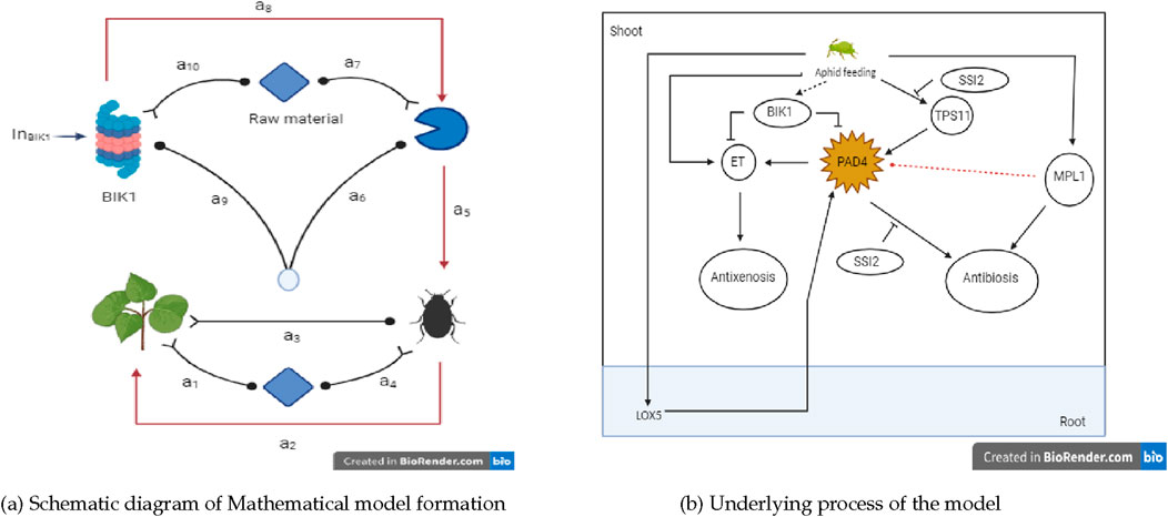
Figure 1. Insights into the plant-insects dynamical model. (A) Schematic diagram of Mathematical model formation. (B) Underlying process of the model.

Table 1

Table 1. Variables of the model.

The key assumptions of the model 1,2 are as follow,

i. The model assumes that the plant biomass (P), insect herbivore density (I), PAD4 protein (PAD4), and BIK1 protein (BIK1) are homogeneously mixed within the environment. This means that these components are evenly distributed, and their interactions occur uniformly throughout the system.

ii. The environmental conditions, such as temperature, humidity, and nutrient availability, are assumed to be constant.

iii. The model considers a closed system with no immigration or emigration of insect herbivores. The population dynamics of the insect herbivores are governed solely by the birth and death rates within the system.

iv. The concentration of the BIK1 inhibitor $({\text{In}}_{\text{BIK}1})$ is assumed to be constant and does not change over time.

v. The rate constants $(a_i)$ and carrying capacity $(K)$ are assumed to be constant over time.

vi. The model does not consider time delays in the responses of the components. All interactions and changes occur instantaneously.

vii. The model assumes that there are no external interventions, such as pesticide applications or genetic modifications.

3 Qualitative analysis of the model

3.1 Existence and uniqueness of the solution

The following section provides existence, boundedness, and equilibrium analysis for the current model. Theorem 3.1 ensures that the interactions between variables of the system are well-defined and consistent under all modeled conditions, making the system biologically predictable. While the approach used here is specific to our system, similar results in other contexts can be found in [28, 29].

Theorem 3.1. For system 1, there exists a unique solution.

Proof. The proof is given in appendix section (Theorem 3.1).

Theorem 3.2. The solutions of the system 1 are bounded for all $t\ge 0$.

Proof. The proof is given in appendix section (Theorem 3.1). Theorem 3.2 reflects that the population levels of plants, insects, and proteins will not grow indefinitely or collapse to zero, showing the natural limits on growth due to environmental factors and resource constraints. The proof is given in appendix section (Theorem 3.2).

3.2 Equilibrium analysis

In this section, we analyze the equilibrium points of the system and assess their stability. The variational matrix is a matrix of first-order partial derivatives that encapsulates the local linearization of a nonlinear dynamical system around its equilibrium points. If the system is described by a set of ordinary differential equations $\dot{\mathbf{y}}=f(\mathbf{y})$, where $\mathbf{y}=(y_1,y_2,\dots ,y_n)$ represents the state variables, the variational matrix $V$ is given by,

$V=\frac{\partial f\left(\mathbf{y}\right)}{\partial \mathbf{y}}=\left(\begin{array}{cccc}\hfill \frac{\partial f_1}{\partial y_1}\hfill & \hfill \frac{\partial f_1}{\partial y_2}\hfill & \hfill \dots \hfill & \hfill \frac{\partial f_1}{\partial y_n}\hfill \\ \hfill \frac{\partial f_2}{\partial y_1}\hfill & \hfill \frac{\partial f_2}{\partial y_2}\hfill & \hfill \dots \hfill & \hfill \frac{\partial f_2}{\partial y_n}\hfill \\ \hfill ⋮\hfill & \hfill ⋮\hfill & \hfill \ddots \hfill & \hfill ⋮\hfill \\ \hfill \frac{\partial f_n}{\partial y_1}\hfill & \hfill \frac{\partial f_n}{\partial y_2}\hfill & \hfill \dots \hfill & \hfill \frac{\partial f_n}{\partial y_n}\hfill \end{array}\right).$

This matrix captures the infinitesimal behavior of the system around the equilibrium points by linearizing the system. The eigenvalue spectrum of the variational matrix governs the local stability properties of the equilibrium. If all eigenvalues have negative real parts, the system exhibits asymptotic stability at the equilibrium point. If any eigenvalue has a positive real part, the equilibrium is unstable. The variational matrix of our model is given by,

$V=\left(\begin{array}{cccc}\hfill a_1\left(1-\frac{2}{K}\right)-a_2\hfill & \hfill -a_2\hfill & \hfill 0\hfill & \hfill 0\hfill \\ \hfill a_3\hfill & \hfill a_3-a_4-a_5\hfill & \hfill -a_5\hfill & \hfill 0\hfill \\ \hfill a_6\hfill & \hfill a_6\hfill & \hfill -a_7-a_8\hfill & \hfill -a_8\hfill \\ \hfill a_9\hfill & \hfill a_9\hfill & \hfill 0\hfill & \hfill -a_{10}\hfill \end{array}\right).$

3.2.1 ${\mathcal{E}}_1(\mathrm{0,0,0,0})$

The variational matrix $V$ at ${\mathcal{E}}_1(\mathrm{0,0,0,0})$ is,

$V{|}_{{\mathcal{E}}_1\left(\mathrm{0,0,0,0}\right)}=\left(\begin{array}{cccc}\hfill a_1\hfill & \hfill 0\hfill & \hfill 0\hfill & \hfill 0\hfill \\ \hfill 0\hfill & \hfill -a_4\hfill & \hfill 0\hfill & \hfill 0\hfill \\ \hfill 0\hfill & \hfill 0\hfill & \hfill -a_7\hfill & \hfill 0\hfill \\ \hfill 0\hfill & \hfill 0\hfill & \hfill 0\hfill & \hfill -a_{10}\hfill \end{array}\right).$

So, the eigenvalues at the equilibrium point ${\mathcal{E}}_1(\mathrm{0,0,0,0})$ are,

${\lambda }_1=a_1,{\lambda }_2=-a_4,{\lambda }_3=-a_7,{\lambda }_4=-a_{10}$

Theorem 3.3. The equilibrium point ${\mathcal{E}}_1(\mathrm{0,0,0,0})$ is locally asymptotically stable, if $a_1<0$.

Proof. The proof is easy to follow.

3.2.2 ${\mathcal{E}}_2(\mathrm{1,0,0,0})$

The variational matrix $V$ at ${\mathcal{E}}_2(\mathrm{1,0,0,0})$ is,

$V{|}_{{\mathcal{E}}_2\left(\mathrm{1,0,0,0}\right)}=\left(\begin{array}{cccc}\hfill a_1\left(1-\frac{2}{K}\right)\hfill & \hfill -a_2\hfill & \hfill 0\hfill & \hfill 0\hfill \\ \hfill 0\hfill & \hfill a_3-a_4\hfill & \hfill 0\hfill & \hfill 0\hfill \\ \hfill 0\hfill & \hfill a_6\hfill & \hfill -a_7\hfill & \hfill 0\hfill \\ \hfill 0\hfill & \hfill a_9\hfill & \hfill 0\hfill & \hfill -a_{10}\hfill \end{array}\right).$

So, the eigenvalues at the equilibrium point ${\mathcal{E}}_2(\mathrm{1,0,0,0})$ are,

${\lambda }_1=a_1\left(1-\frac{2}{K}\right),{\lambda }_2=a_3-a_4,{\lambda }_3=-a_7,{\lambda }_4=-a_{10}$

Theorem 3.4. The equilibrium point ${\mathcal{E}}_2(\mathrm{1,0,0,0})$ is locally asymptotically stable, if $K<2$ and $a_1<a_2$ or $a_3<a_4+a_5$.

Proof. The proof is easy to follow.

3.2.3 ${\mathcal{E}}_3(\mathrm{0,1,0,0})$

The variational matrix for ${\mathcal{E}}_3(\mathrm{0,1,0,0})$ is,

$V{|}_{{\mathcal{E}}_3\left(\mathrm{0,1,0,0}\right)}=\left(\begin{array}{cccc}\hfill a_1-a_2\hfill & \hfill 0\hfill & \hfill 0\hfill & \hfill 0\hfill \\ \hfill a_3\hfill & \hfill -a_4\hfill & \hfill -a_5\hfill & \hfill 0\hfill \\ \hfill a_6\hfill & \hfill 0\hfill & \hfill -a_7\hfill & \hfill 0\hfill \\ \hfill a_9\hfill & \hfill 0\hfill & \hfill 0\hfill & \hfill -a_{10}\hfill \end{array}\right).$

The eigenvalues are for the equilibrium point ${\mathcal{E}}_3(\mathrm{0,1,0,0})$ are,

${\lambda }_1=a_1-a_2,{\lambda }_2=-a_4,{\lambda }_3=-a_7,{\lambda }_4=-a_{10}$

Theorem 3.5. The equilibrium point ${\mathcal{E}}_3(\mathrm{0,1,0,0})$ is locally asymptotically stable, if $a_1<a_2$.

Proof. The proof is easy to follow.

3.2.4 ${\mathcal{E}}_4(\mathrm{0,0,1,0})$

The variational matrix for ${\mathcal{E}}_4(\mathrm{0,0,1,0})$ is,

$V{|}_{{\mathcal{E}}_4\left(\mathrm{0,0,1,0}\right)}=\left(\begin{array}{cccc}\hfill a_1\hfill & \hfill 0\hfill & \hfill 0\hfill & \hfill 0\hfill \\ \hfill 0\hfill & \hfill -a_4-a_5\hfill & \hfill 0\hfill & \hfill 0\hfill \\ \hfill 0\hfill & \hfill 0\hfill & \hfill -a_7\hfill & \hfill -a_8\hfill \\ \hfill 0\hfill & \hfill 0\hfill & \hfill 0\hfill & \hfill -a_{10}\hfill \end{array}\right).$

The eigenvalues are for the equilibrium point ${\mathcal{E}}_4(\mathrm{0,0,1,0})$ are,

${\lambda }_1=a_1,{\lambda }_2=-a_4-a_5,{\lambda }_3=-a_7,{\lambda }_4=-a_{10}$

Theorem 3.6. The equilibrium point ${\mathcal{E}}_4(\mathrm{0,0,1,0})$ is locally asymptotically stable, if $a_1<0$.

Proof. The proof is easy to follow.

3.2.5 ${\mathcal{E}}_5(\mathrm{0,0,0,1})$

The variational matrix for ${\mathcal{E}}_5(\mathrm{0,0,0,1})$ is,

$V{|}_{{\mathcal{E}}_5\left(\mathrm{0,0,0,1}\right)}=\left(\begin{array}{cccc}\hfill a_1\hfill & \hfill 0\hfill & \hfill 0\hfill & \hfill 0\hfill \\ \hfill 0\hfill & \hfill -a_4\hfill & \hfill 0\hfill & \hfill 0\hfill \\ \hfill 0\hfill & \hfill 0\hfill & \hfill -a_7-a_8\hfill & \hfill 0\hfill \\ \hfill 0\hfill & \hfill 0\hfill & \hfill 0\hfill & \hfill -a_{10}\hfill \end{array}\right).$

The eigenvalues are for the equilibrium point ${\mathcal{E}}_5(\mathrm{0,0,0,1})$ are,

${\lambda }_1=a_1,{\lambda }_2=-a_4,{\lambda }_3=-a_7-a_8,{\lambda }_4=-a_{10}$

Theorem 3.7. The equilibrium point ${\mathcal{E}}_5(\mathrm{0,0,0,1})$ is locally asymptotically stable, if $a_1<0$.

Proof. The proof is easy to follow.

3.2.6 ${\mathcal{E}}_6(\mathrm{1,1,0,0})$

The variational matrix for ${\mathcal{E}}_6(\mathrm{0,0,0,1})$ is,

$V{|}_{{\mathcal{E}}_6\left(\mathrm{1,1,0,0}\right)}=\left(\begin{array}{cccc}\hfill a_1\left(1-\frac{2}{K}\right)-a_2\hfill & \hfill -a_2\hfill & \hfill 0\hfill & \hfill 0\hfill \\ \hfill a_3\hfill & \hfill a_3-a_4\hfill & \hfill 0\hfill & \hfill 0\hfill \\ \hfill a_6\hfill & \hfill a_6\hfill & \hfill -a_7\hfill & \hfill 0\hfill \\ \hfill a_9\hfill & \hfill a_9\hfill & \hfill 0\hfill & \hfill -a_{10}\hfill \end{array}\right).$

The eigenvalues are for the equilibrium point ${\mathcal{E}}_6(\mathrm{1,1,0,0})$ are,

${\lambda }_1=a_1\left(1-\frac{2}{K}\right)-a_2,{\lambda }_2=a_3-a_4,{\lambda }_3=-a_7,{\lambda }_4=-a_{10}$

Theorem 3.8. The equilibrium point ${\mathcal{E}}_6(\mathrm{1,1,0,0})$ is locally asymptotically stable, if $a_1\left(1-\frac{2}{K}\right)<a_2$ and $a_3<a_4$.

Proof. The proof is easy to follow.

3.2.7 ${\mathcal{E}}_7(\mathrm{1,0,1,0})$

The variational matrix at ${\mathcal{E}}_7(\mathrm{1,0,1,0})$ is,

$V{|}_{{\mathcal{E}}_7\left(\mathrm{1,0,1,0}\right)}=\left(\begin{array}{cccc}\hfill a_1\left(1-\frac{2}{K}\right)\hfill & \hfill 0\hfill & \hfill 0\hfill & \hfill 0\hfill \\ \hfill 0\hfill & \hfill -a_4-a_5\hfill & \hfill 0\hfill & \hfill 0\hfill \\ \hfill 0\hfill & \hfill a_6\hfill & \hfill -a_7\hfill & \hfill 0\hfill \\ \hfill 0\hfill & \hfill 0\hfill & \hfill 0\hfill & \hfill -a_{10}\hfill \end{array}\right).$

The eigenvalues are for the equilibrium point ${\mathcal{E}}_7(\mathrm{1,0,1,0})$ are,

${\lambda }_1=a_1\left(1-\frac{2}{K}\right),{\lambda }_2=-a_4-a_5,{\lambda }_3=-a_7,{\lambda }_4=-a_{10}$

Theorem 3.9. The equilibrium point ${\mathcal{E}}_7(\mathrm{1,1,0,0})$ is locally asymptotically stable, if $1-\frac{2}{K}<0$ (i.e., $K<2$).

Proof. The proof is easy to follow.

3.2.8 ${\mathcal{E}}_8(\mathrm{1,0,1,1})$

The variational matrix at ${\mathcal{E}}_8(\mathrm{1,0,1,1})$ is,

$V{|}_{{\mathcal{E}}_8\left(\mathrm{1,0,1,1}\right)}=\left(\begin{array}{cccc}\hfill a_1\left(1-\frac{2}{K}\right)\hfill & \hfill 0\hfill & \hfill 0\hfill & \hfill 0\hfill \\ \hfill 0\hfill & \hfill -a_4-a_5\hfill & \hfill 0\hfill & \hfill 0\hfill \\ \hfill 0\hfill & \hfill a_6\hfill & \hfill -a_7-a_8\hfill & \hfill -a_8\hfill \\ \hfill 0\hfill & \hfill 0\hfill & \hfill 0\hfill & \hfill -a_{10}\hfill \end{array}\right).$

The eigenvalues are for the equilibrium point ${\mathcal{E}}_8(\mathrm{1,0,1,1})$ are,

${\lambda }_1=a_1\left(1-\frac{2}{K}\right),{\lambda }_2=-a_4-a_5,{\lambda }_3=-a_7-a_8,{\lambda }_4=-a_{10}$

Theorem 3.10. The equilibrium point ${\mathcal{E}}_8(\mathrm{1,0,1,1})$ is locally asymptotically stable, if $1-\frac{2}{K}<0$ (i.e., $K<2$).

Proof. The proof is easy to follow.

3.3 Biological significance

The equilibrium analysis emphasizes the essential dynamics between plant biomass, insect herbivores, and defense proteins, PAD4 and BIK1, in maintaining ecological stability. Theorems 3.4, 3.5 establish the foundational roles of plants and insects in the system, highlighting how their coexistence is necessary for sustaining balanced populations. The most biologically significant results are demonstrated in Theorems 3.9, 3.10, where plants maintain stable coexistence with PAD4 or both PAD4 and BIK1 proteins. These equilibria reflect the plant’s defensive mechanisms being actively regulated by these proteins, ensuring preparedness for potential herbivore attacks. Theorem 3.8 presents the ecologically balanced state, where both plants and insect herbivores coexist, with PAD4 and BIK1 proteins playing a regulatory role. This equilibrium ensures that plant defense systems, driven by these proteins, manage herbivore populations effectively, maintaining system stability. This section highlights the crucial role of plant defense proteins in regulating insect interactions, ensuring long-term ecological balance.

3.4 Basic reproduction number

The basic reproduction number $R_0$ is given by,

$R_0=\frac{a_{3}K}{a_4}.$

Theorem 3.11. If $R_0>1$, then the system is uniformly persistent, meaning there exists a positive constant $\delta$ such that for any solution $(y_1(t),y_2(t),y_3(t),y_4(t))$ with initial conditions in the interior of the positive orthant, we have,

Proof. The proof is given in appendix (Theorem 3.11).

$\underset{t\to \infty }{\mathrm{lim\; inf}}{y}_i\left(t\right)\ge \delta >0,\mathit{\text{for}}i=\mathrm{1,2,3,4}.$

3.5 Stochastic analysis

For stochastic system with $y_1,y_2,y_3,y_4$, we define $\mathrm{\Gamma }$ as

$\mathrm{\Gamma }=\left\{\left(y_1\left(t\right),y_2\left(t\right),y_3\left(t\right),y_4\left(t\right)\right)\in {\mathbb{R}}_{+}^4:y_1\left(t\right)+y_2\left(t\right)+y_3\left(t\right)+y_4\left(t\right)\le \frac{a_1}{a_2}\right\}$

We need to show that $\mathrm{\Gamma }$ fulfills almost sure invariance principle.

Theorem 3.12. The closed set $\mathrm{\Gamma }$ fulfills almost sure invariance principle for the stochastic system 2.

Proof. This theorem guarantees that the system remains within realistic bounds even under stochastic influences, indicating that the ecosystem is robust to fluctuations in population and protein levels. The proof is given in appendix section (Theorem 3.12).

Theorem 3.13. For $(y_1(0),y_2(0),y_3(0),y_4(0))\in \mathrm{\Gamma }$, system 2 has a unique and positive solution almost surely.

Proof. This theorem assures that despite randomness, the system’s biological variables (plants, insects, proteins) maintain positive values, ensuring the ecological system remains functional. The proof is given in appendix section (Theorem 3.13).

4 Numerical simulations

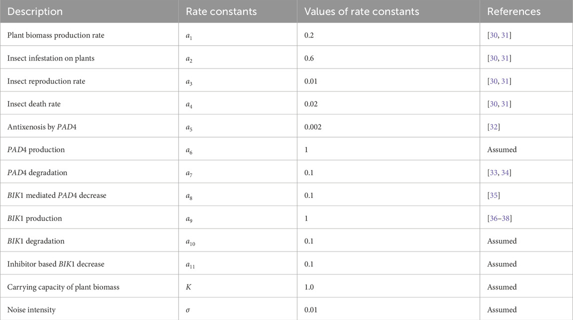
In the following subsections, various numerical results are provided. The values of the parameters used in the model are given in Table 2. The Euler-Maruyama method is used to solve the stochastic differential equations iteratively as follow,

$\begin{array}{ll}\hfill y_1\left(t+\mathrm{\Delta }t\right)& =y_1\left(t\right)+\left(k_1{y}_1\left(t\right)\left(1-\frac{y_1\left(t\right)}{K}\right)-k_2{y}_1\left(t\right)y_2\left(t\right)\right)\mathrm{\Delta }t+\sigma \sqrt{\mathrm{\Delta }t}\cdot {\eta }_1\left(t\right),\hfill \\ \hfill y_2\left(t+\mathrm{\Delta }t\right)& =y_2\left(t\right)+\left(k_3{y}_1\left(t\right)y_2\left(t\right)-k_4{y}_2\left(t\right)-k_5{y}_3\left(t\right)y_2\left(t\right)\right)\mathrm{\Delta }t+\sigma \sqrt{\mathrm{\Delta }t}\cdot {\eta }_2\left(t\right),\hfill \\ \hfill y_3\left(t+\mathrm{\Delta }t\right)& =y_3\left(t\right)+\left(k_6{y}_1\left(t\right)y_2\left(t\right)-k_7{y}_3\left(t\right)-k_8{y}_3\left(t\right)y_4\left(t\right)\right)\mathrm{\Delta }t+\sigma \sqrt{\mathrm{\Delta }t}\cdot {\eta }_3\left(t\right),\hfill \\ \hfill y_4\left(t+\mathrm{\Delta }t\right)& =y_4\left(t\right)+\left(k_9{y}_1\left(t\right)y_2\left(t\right)-k_{10}{y}_4\left(t\right)-k_{11}\cdot 0.1\right)\mathrm{\Delta }t+\sigma \sqrt{\mathrm{\Delta }t}\cdot {\eta }_4\left(t\right),\hfill \end{array}$

where ${\eta }_i(t)$ represents the noise term. For Gaussian noise, ${\eta }_i(t)$ is from a normal distribution $\mathcal{N}(\mathrm{0,1})$,

${\eta }_i\left(t\right)\sim \mathcal{N}\left(\mathrm{0,1}\right).$

Table 2

Table 2. Parameter values used in the model.

For Lévy noise, ${\eta }_i(t)$ is from a Lévy distribution.

${\eta }_i\left(t\right)\sim \text{Lvy}\left(\alpha ,\beta \right).$

where,

$\mathrm{\Delta }{W}_t\sim \mathcal{N}\left(0,\mathrm{\Delta }t\right).$

And

$\mathrm{\Delta }{W}_t=\sqrt{\mathrm{\Delta }t}\cdot Z,$

where $Z$ is a standard normal random variable $(Z\sim \mathcal{N}(\mathrm{0,1}))$.

4.1 Noises comparison

Figure 2A shows the dynamics of plant biomass $(y_1)$ under deterministic, Gaussian, and Lévy noise conditions. Under deterministic conditions, plant biomass follows a smooth decline and recovery trajectory. When Gaussian noise is introduced, the system exhibits more fluctuations compared to the deterministic case but maintains a generally similar trend. Lévy noise, however, results in significantly larger fluctuations, reflecting more extreme variations in plant biomass. This observation is consistent with findings from the study [39], which highlighted the importance of Lévy noise in capturing extreme events in biological systems.

Figure 2

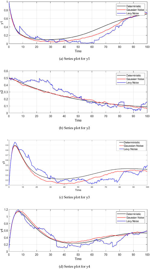
Figure 2. Time series plots of the system variables under different noise conditions (deterministic, Gaussian, and Lévy noise). For all variables—plant biomass $(y_1)$, insect herbivore density $(y_2)$, PAD4 levels $(y_3)$, and BIK1 levels $(y_4)$ deterministic conditions show smooth trends, Gaussian noise introduces minor fluctuations, and Lévy noise results in more extreme variations and larger deviations. (A) Series plot for y1. (B) Series plot for y2. (C) Series plot for y3. (D) Series plot for y4.

The dynamics of insect herbivore density $(y_2)$ under different noise conditions are illustrated in Figure 2B. Deterministic conditions show a continuous decline in insect density. Gaussian noise introduces more variability into the system, causing minor fluctuations around the declining trend. Lévy noise, on the other hand, introduces significant variability, leading to more pronounced fluctuations in insect density. The same trend is followed by other variables (Figures 2C, D).

The parameter $a_1$ significantly impacts plant biomass $y_1$ (Figure 3A). Higher values of $a_1$ indicate better soil conditions and other suitable conditions, allowing plants to maintain or increase their biomass over time.

Figure 3

Figure 3. Effect of plant biomass production constant.

4.2 Lévy noise

The insect herbivore density $(y_2)$ exhibits distinct behaviors under different noise intensities (Figure 4). At low noise intensity $(\sigma =0.01)$ (Figure 4A), the herbivore density decreases steadily, closely mirroring the deterministic model. However, as noise intensity increases, particularly at moderate levels $(\sigma =0.05)$ (Figure 4B), there is an observable increase in fluctuations around the declining trend.

Figure 4

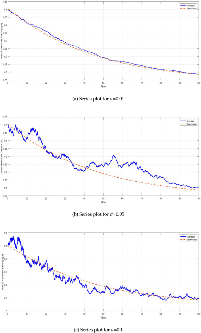
Figure 4. Time series of insect herbivore density $(y_2)$ under different noise intensities. With higher noise intensity $(\sigma =0.1)$, the fluctuations are significantly larger, leading to increased variability in the system’s behavior. (A) Series plot for σ=0.01. (B) Series plot for σ=0.05. (C) Series plot for σ=0.1.

Similarly, the $PAD4$ levels $(y_3)$ show an interesting pattern under varying noise intensities (Figure 5). At a moderate noise intensity of $\sigma =0.05$ (Figure 5A), PAD4 levels maintain a relatively stable and higher average compared to both lower and higher noise intensities. This stability at moderate noise levels suggests that the system can better sustain its defense mechanisms, making this noise intensity particularly beneficial for maintaining $PAD4$ activity. Conversely, at higher noise intensities $(\sigma =0.1)$ (Figure 5C), PAD4 levels decrease significantly, indicating that excessive noise can disrupt the plant’s defense responses.

Figure 5

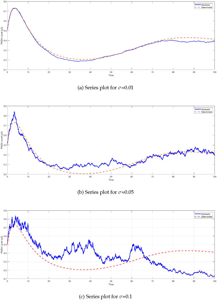
Figure 5. Time series of PAD4 protein levels $(y_3)$ under different noise intensities. With higher noise intensity $(\sigma =0.1)$, significant fluctuations occur, showing increased sensitivity to the noise. (A) Series plot for σ=0.01. (B) Series plot for σ=0.05. (C) Series plot for σ=0.1.

The comparison between the deterministic and stochastic models reveals critical insights into the behavior of the system under different noise intensities (Figure 6). One of the most notable observations is the impact of stochasticity on the $BIK1$ levels $(y_4)$. As noise intensity increases, $BIK1$ levels exhibit significant fluctuations. For higher noise intensities, $BIK1$ levels decrease more rapidly, indicating that the stochastic model is more sensitive to perturbations. This sensitivity suggests that in real-world scenarios, $BIK1$ levels are likely to be more variable due to environmental and internal noise, which the deterministic model fails to capture (Figures 6A–C) [40, 41].

Figure 6

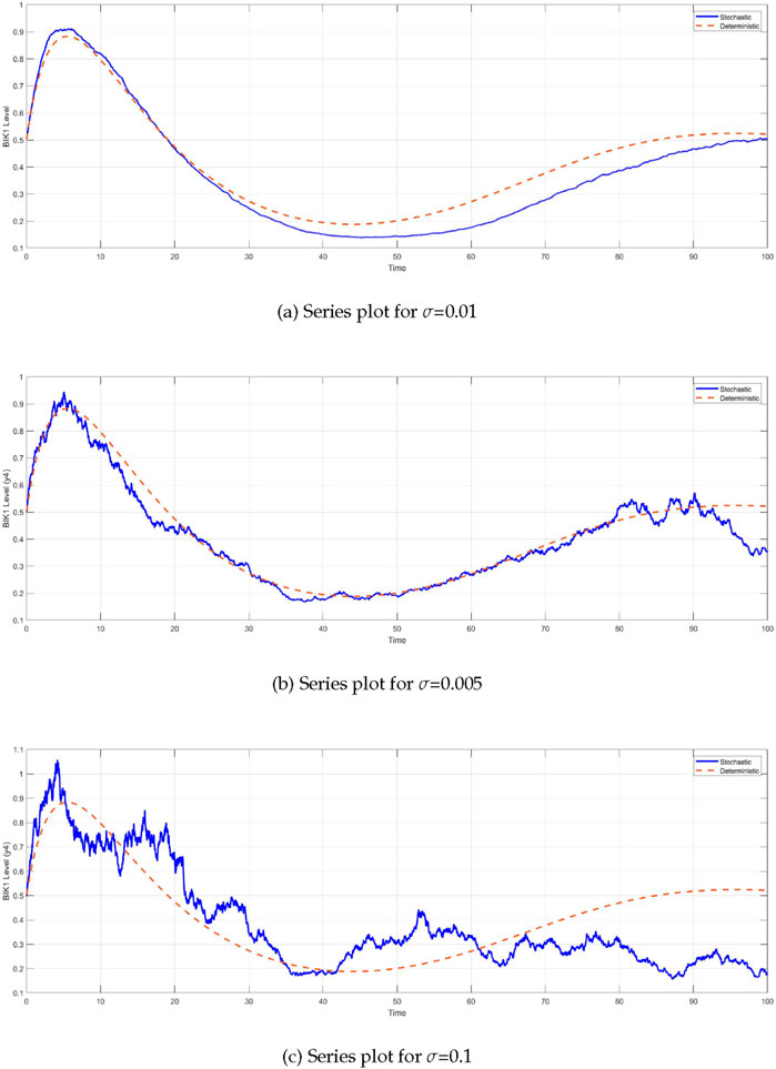
Figure 6. Time series of BIK1 protein levels $(y_4)$ under different noise intensities. At higher noise intensity $(\sigma =0.1)$, the system exhibits large variability, indicating a stronger response to the perturbations. (A) Relationship between PAD4 Levels (y3) and BIK1 Levels (y4). (B) Relationship between Plant Biomass (y1) and Insect Herbivore Density (y2).

4.3 Queir plots

Queir plots visually represent how the states of a system evolve over time, especially in complex, nonlinear systems. These plots show the system’s trajectory or path in a simplified, multi-dimensional space, focusing on key variables.

Theorem 4.1. Consider the system defined by,

$\frac{d{y}_1}{dt}=a_1{y}_1\left(1-\frac{y_1}{K}\right)-a_2{y}_1{y}_2.$

If $y_2(t)\le \frac{a_1}{a_2}\left(1-\frac{y_1}{K}\right)$, the plant biomass $y_1(t)$ will grow.

Proof. The proof is given in appendix section (Theorem 4.1).

Theorem 4.2. Consider the system defined by,

$\frac{d{y}_3}{dt}=a_6{y}_1{y}_2-a_7{y}_3-a_8{y}_3{y}_4,$

$\frac{d{y}_4}{dt}=a_9{y}_1{y}_2-a_{10}{y}_4-a_{11}\cdot {\mathit{\text{In}}}_{\mathit{\text{BIK}}1}.$

If $y_1{y}_2$ exceeds the thresholds $\frac{a_7{y}_3+a_8{y}_3{y}_4}{a_6}$ and $\frac{a_{10}{y}_4+a_{11}\cdot {In}_{BIK1}}{a_9}$, both $y_3(t)$ and $y_4(t)$ will increase, contributing to the plant’s defensive response.

Proof. The proof is given in appendix section (Theorem 4.2).

4.3.1 Relationship between $PAD4$ levels $(y_3)$ and $BIK1$ levels $(y_4)$

As shown in Figure 7A, the relationship between $PAD4$ $(y_3)$ and $BIK1$ $(y_4)$ levels exhibits a complex trend where increases in $PAD4$ lead to increases in $BIK1$ up to a threshold, after which the relationship stabilizes. This pattern reflects regulatory feedback mechanisms, where $PAD4$ activation upregulates $BIK1$ until feedback stabilization occurs. The findings align with studies on plant signaling pathways, where $BIK1$ is essential in defense responses, and stochastic dynamics impact regulatory networks.

Figure 7

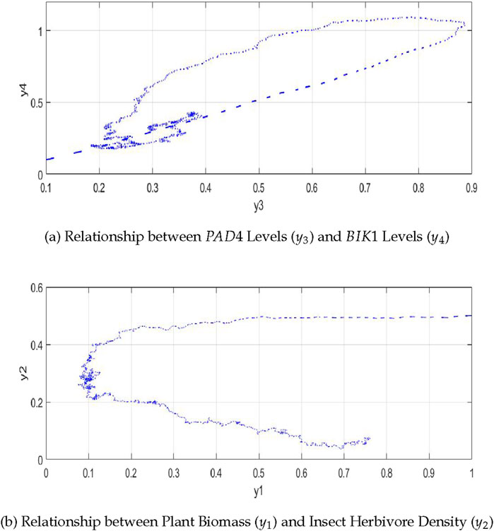
Figure 7. The plot shows the relationships in the plant-insect interaction model: (A) between $PAD4$ Levels $(y_3)$ and $BIK1$ Levels $(y_4)$, and (B) between Plant Biomass $(y_1)$ and Insect Herbivore Density $(y_2)$.

4.3.2 Relationship between plant biomass $(y_1)$ and insect herbivore density $(y_2)$

Figure 7B shows that the relationship between plant biomass $(y_1)$ and insect herbivore density $(y_2)$ is inversely correlated, where increases in plant biomass lead to reductions in herbivore density. This reflects the plant’s defense mechanisms, mediated by proteins like $PAD4$ and $BIK1$, which regulate herbivore populations. Stochastic fluctuations observed are consistent with known plant-herbivore interaction models.

4.4 Probability density distributions

The stationary distribution describes the long-term behavior of a stochastic process, offering insights into the stability of system. A Markov process, which models a sequence of potential events, is primarily influenced by the state attained in the previous event. In simpler terms, it can be thought of as “what happens in the future depends only on the current situation.”

In the space ${\mathbb{R}}_{+}^m$, consider that the process $\mathbf{J}(t)$ is regular and time-homogeneous, exhibiting Markovian behavior with respect to time $t$ of the form:

$\text{d}\mathbf{J}\left(t\right)={\displaystyle \sum _{s=1}^l}{\kappa }_s\text{d}{\mathcal{B}}_s\left(t\right)+b\left(\mathbf{J}\right)\text{d}t.$

Here, $\mathcal{A}(\mathbf{J})=[{\iota }_{ij}(y)]$ is the matrix associated with the mixing terms, where ${\iota }_{ij}(y)={\sum }_{s=1}^l{\kappa }_s^i(y){\kappa }_s^j(y)$.

Lemma 4.1. [42, 43] The process $\mathbf{J}(t)$ is said to possess a unique stationary distribution $m(\cdot )$ if we can identify a bounded domain with regular boundaries $U,\bar{U}\subset {\mathbb{R}}^d$, such that,

1. The smallest eigenvalue of $\mathcal{A}(t)$ is bounded away from zero within the domain $U$ and its vicinity.

Additionally, if $y\in {\mathbb{R}}^d\backslash U$, the mean time $\tau$ (at which a path originating from $y$ reaches $U$) is finite, and ${\sup }_{y\in L}\mathbb{E}\tau <\infty$ for each compact subset $L\subset {\mathbb{R}}^m$. Furthermore, let $g(\cdot )$ be an integrable function with respect to the measure $\pi$, then

$\underset{T\to \infty }{\lim }\frac{1}{T}{\int }_0^{T}f\left({\mathbf{J}}_y\left(t\right)\right)\text{d}t={\int }_{{\mathbb{R}}^d}g\left(y\right)\pi \left(\text{d}y\right)=1\text{for\hspace{0.17em}all\hspace{0.17em}}y\in {\mathbb{R}}^d.$

we define,

${\mathcal{R}}_0^p=\frac{a_1{a}_3{a}_6}{\left(a_2+\frac{{\zeta }_1^2}{2}\right)\left(a_4+\frac{{\zeta }_2^2}{2}\right)\left(a_7+\frac{{\zeta }_3^2}{2}\right)\left(a_{10}+\frac{{\zeta }_4^2}{2}\right)}.(3)$

Theorem 4.3. For $(y_1(0),y_2(0),y_3(0),y_4(0))\in \mathrm{\Gamma }$, the system has a unique stationary distribution $\pi (.)$ as well as the solution $(y_1(t),y_2(t),y_3(t),y_4(t))$ to the model is ergodic in nature.

Proof. The proof is given in appendix section (Theorem 4.3).

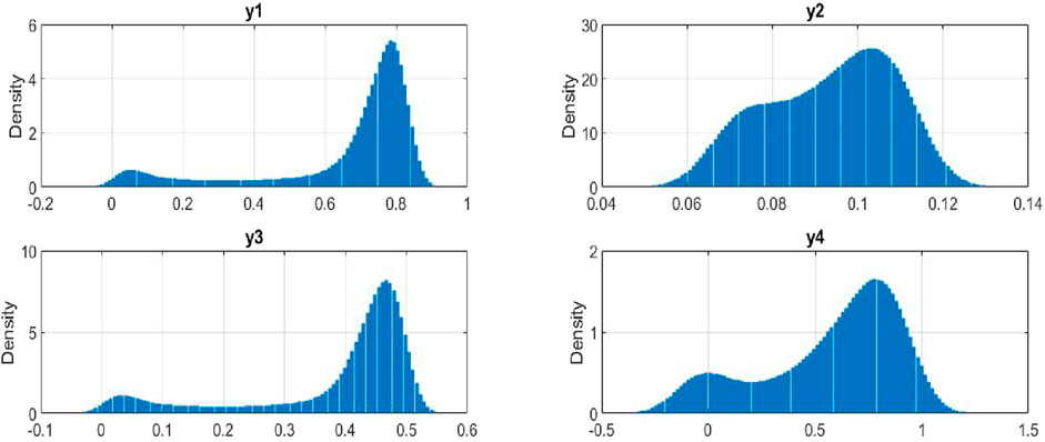
Figure 8 presents the probability density distributions for the key variables in our stochastic model of plant-insect interactions. The density of $y_1$ (is predominantly concentrated around 0.5, indicating that this is the most common biomass level. $y_2$ exhibits its highest density at approximately 0.1, showing that insect populations reach this density influenced by factors such as available plant biomass and natural predator presence. For $y_3$, the density peaks sharply, demonstrating that $PAD4$ protein levels consistently reach an optimal level for effective response to insect herbivory. In contrast, $y_4$ displays a bimodal distribution, indicating two dominant states of this protein. The lower levels of $BIK1$, corresponding to the first peak, are associated with heightened $PAD4$ activity, reflecting a robust plant defense mechanism. The second peak at higher $BIK1$ levels suggests a regulatory balance where $BIK1$ moderates the defense response to prevent overreaction.

Figure 8

Figure 8. Density Distribution of the model variable’s.

5 MEMs in control

The integration of Micro-Electromechanical Systems (MEMS) in plant systems has revolutionized the field of precision agriculture by providing real-time monitoring and adaptive control capabilities. MEMS sensors are widely used for tracking environmental parameters such as soil moisture, temperature, humidity, and nutrient levels, enabling more efficient and precise irrigation and fertilization strategies. For example, The increasing demand for the miniaturization of biosensors has driven growing interest in microelectromechanical systems (MEMS) [44, 45], along with nanoelectromechanical systems (NEMS) and microfluidic or lab-on-a-chip based biosensors [35, 46]. These compact systems provide enhanced accuracy, sensitivity, specificity, and cost-efficiency, while also offering high-performance biosensing capabilities. MEMS-based biosensors leverage a range of detection methods, including optical, mechanical, magnetic, and electrochemical approaches. For optical detection, probes like organic dyes, semiconductor quantum dots, and other fluorescence markers are commonly employed. In magnetic MEMS biosensors, nanoparticles such as magnetic, paramagnetic, or ferromagnetic particles are utilized. Mechanical MEMS biosensors operate based on changes in surface stress or mass [47], where biochemical reactions or analyte adsorption on the cantilever induce surface stress changes. Electrochemical MEMS biosensors, on the other hand, rely on amperometric, potentiometric, or conductometric detection methods [48–51]. For each variable, sensor-based feedback terms can be introduced to adjust the differential equations based on real-time data gathered by MEMS. This can include intervention strategies or feedback loops that modify plant biomass growth, herbivore density, and molecular signals. We extend the stochastic Equation 2 to include MEMS input, denoted by a new variable $M(t)$, representing MEMS sensor feedback,

$d{y}_1=\left(a_1{y}_1\left(1-\frac{y_1}{K}\right)-a_2{y}_1{y}_2+M_1\left(t\right)\right)dt+{\sigma }_1{y}_{1}d{W}_1,$

$d{y}_2=\left(a_3{y}_1{y}_2-a_4{y}_2-a_5{y}_3{y}_2+M_2\left(t\right)\right)dt+{\sigma }_2{y}_{2}d{W}_2,$

$d{y}_3=\left(a_6{y}_1{y}_2-a_7{y}_3-a_8{y}_3{y}_4+M_3\left(t\right)\right)dt+{\sigma }_3{y}_{3}d{W}_3,$

$d{y}_4=\left(a_9{y}_1{y}_2-a_{10}{y}_4-a_{11}\cdot I{n}_{\mathit{BIK1}}+M_4\left(t\right)\right)dt+{\sigma }_4{y}_{4}d{W}_4.$

For each variable $y_i(t)$, the MEMS feedback terms $M_i(t)$ are defined as follows,

$M_1\left(t\right)={\beta }_1\cdot \text{Control\hspace{0.17em}Function\hspace{0.17em}for\hspace{0.17em}}{y}_1\left(t\right),$

$M_2\left(t\right)={\beta }_2\cdot \text{Control\hspace{0.17em}Function\hspace{0.17em}for\hspace{0.17em}}{y}_2\left(t\right),$

$M_3\left(t\right)={\beta }_3\cdot \text{Control\hspace{0.17em}Function\hspace{0.17em}for\hspace{0.17em}}{y}_3\left(t\right),$

$M_4\left(t\right)={\beta }_4\cdot \text{Control\hspace{0.17em}Function\hspace{0.17em}for\hspace{0.17em}}{y}_4\left(t\right).$

The parameters ${\beta }_1,{\beta }_2,{\beta }_3$, and ${\beta }_4$ represent scaling factors that control the strength of the feedback applied by the MEMS sensors for each variable. Figure 9 presents the results incorporating MEMS feedback into the system. In 5, the plant biomass $y_1$ shows a significant oscillatory behavior in the stochastic case, with a generally increasing trend after an initial decline. The MEMS feedback helps stabilize biomass growth, resulting in quicker recovery compared to the deterministic solution, which shows a smoother, slower increase. In 5, the insect herbivore density $y_2$ demonstrates a steady decline, with MEMS further suppressing insect growth. The stochastic model exhibits more variability and faster suppression of herbivores, while the deterministic model shows a smoother, more gradual reduction. The PAD4 protein dynamics $y_3$ in five show an initial peak followed by a decline and eventual stabilization, with MEMS feedback leading to more active and pronounced fluctuations in the stochastic case compared to the smoother deterministic curve. In 5, the BIK1 protein $y_4$ follows a similar trend to the other variables, with MEMS inducing stronger oscillations in the stochastic model, particularly towards the later stages. The deterministic solution, on the other hand, stabilizes more smoothly without such fluctuations. The implementation of MEMS introduces dynamic feedback into the system, leading to faster recovery, better control of herbivore density, and more pronounced fluctuations in protein levels. This highlights MEMS’ effectiveness in dynamically regulating plant-insect interactions and molecular signals.

Figure 9

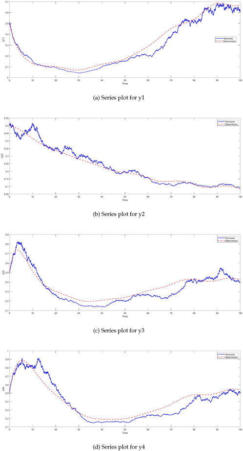
Figure 9. Time series plots of system variables with MEMS feedback under stochastic conditions. For all variables—plant biomass $(y_1)$, insect herbivore density $(y_2)$, PAD4 levels $(y_3)$, and BIK1 levels $(y_4)$—MEMS feedback stabilizes the system’s oscillations. Plant biomass and herbivore density recover more quickly compared to the deterministic case, while PAD4 and BIK1 show increased fluctuations due to dynamic feedback responses. (A) Series plot for y1. (B) Series plot for y2. (C) Series plot for y3. (D) Series plot for y4.

6 Discussion

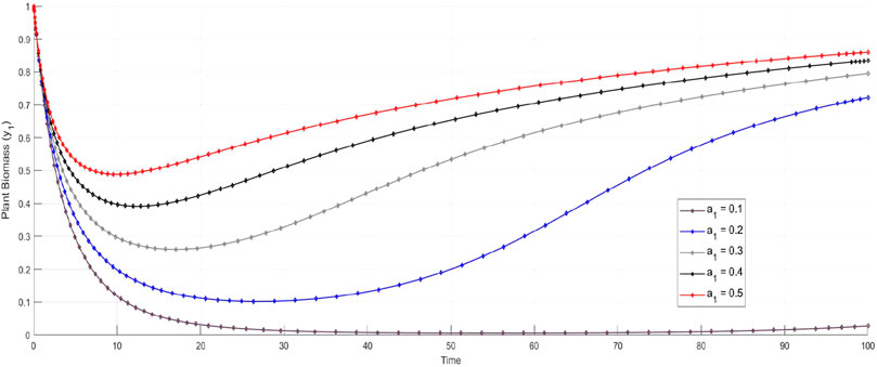
Our comparison of noise conditions revealed distinct behaviors in plant biomass and insect herbivore density. Deterministic conditions produced smooth trajectories, while Gaussian noise caused moderate fluctuations, and Lévy noise led to extreme variations, effectively capturing sudden changes in biological systems. High $PAD4$ levels and low $BIK1$ levels were associated with increased plant biomass and reduced herbivore density, indicating effective plant defense mechanisms. Moderate noise intensity $(\sigma =0.05)$ sustained $PAD4$ activity, providing a balance between system stability and variability.

Lévy noise had a significant impact on $PAD4$ and herbivore density, with moderate noise intensities sustaining $PAD4$ activity for optimal plant defense. Queir plots revealed non-linear regulatory interactions between $PAD4$ and $BIK1$, emphasizing the role of stochastic dynamics in biological networks. The results suggest that moderate noise intensity is optimal for maintaining system function, with MEMS-based feedback showing potential for adaptability by continuously adjusting key parameters.

7 Conclusion

This study provides a comprehensive analysis of the dynamic interactions between plants and insect herbivores, focusing on the molecular interplay between $PAD4$ and $BIK1$ proteins, under various control strategies and noise conditions. The inclusion of different noise types in the model reveals significant insights into the system’s variability. Gaussian noise introduces moderate fluctuations around the deterministic trends, while Lévy noise induces more extreme fluctuations and variability, capturing the sudden changes and extreme events often observed in biological systems. This emphasizes the necessity of incorporating stochastic elements, particularly Lévy noise, to accurately model and understand the complex dynamics of plant-insect interactions. By incorporating MEMS-driven adaptive feedback, we demonstrated how real-time sensor-based interventions can enhance the system’s stability and effectiveness, particularly in maintaining plant health and controlling insect populations under varying noise conditions. Our study advances our understanding of plant-insect interactions and offers valuable insights into the role of noise and control strategies in modulating system behavior. These findings have implications for the development of effective management strategies in agricultural and ecological contexts, paving the way for more robust and sustainable approaches to mitigating the impacts of insect herbivory on plant health and productivity.

Data availability statement

The original contributions presented in the study are included in the article/supplementary material, further inquiries can be directed to the corresponding authors.

Author contributions

QA: Conceptualization, Methodology, Software, Writing–original draft, Writing–review and editing. XQ: Funding acquisition, Project administration, Resources, Visualization, Writing–review and editing. NA: Conceptualization, Data curation, Investigation, Methodology, Writing–review and editing. ZK: Funding acquisition, Project administration, Resources, Supervision, Validation, Visualization, Writing–review and editing.

Funding

The author(s) declare that financial support was received for the research, authorship, and/or publication of this article. This work was supported by the National Natural Science Foundation of China (62172114), the Natural Science Foundation of Guangdong Province of China (2022A1515011468) and the Fundings by Science and Technology Projects in Guangzhou (2023A03J0113).

Acknowledgments

We acknowledge the use of ChatGPT (https://chat.openai.com/) to improve the language.

Conflict of interest

The authors declare that the research was conducted in the absence of any commercial or financial relationships that could be construed as a potential conflict of interest.

Publisher’s note

All claims expressed in this article are solely those of the authors and do not necessarily represent those of their affiliated organizations, or those of the publisher, the editors and the reviewers. Any product that may be evaluated in this article, or claim that may be made by its manufacturer, is not guaranteed or endorsed by the publisher.

Supplementary material

The Supplementary Material for this article can be found online at: https://www.frontiersin.org/articles/10.3389/fphy.2024.1500423/full#supplementary-material

References

1. Girousse C, Moulia B, Silk W, Bonnemain JL. Aphid infestation causes different changes in carbon and nitrogen allocation in alfalfa stems as well as different inhibitions of longitudinal and radial expansion. Plant Physiol (2005) 137(4):1474–84. doi:10.1104/pp.104.057430

PubMed Abstract | CrossRef Full Text | Google Scholar

2. Bos JI, Armstrong MR, Gilroy EM, Boevink PC, Hein I, Taylor RM, et al. Phytophthora infestans effector AVR3a is essential for virulence and manipulates plant immunity by stabilizing host E3 ligase CMPG1. Proc Natl Acad Sci (2010) 107(21):9909–14. doi:10.1073/pnas.0914408107

PubMed Abstract | CrossRef Full Text | Google Scholar

3. De Vos M, Jander G. Myzus persicae (green peach aphid) salivary components induce defence responses in Arabidopsis thaliana. Plant Cell and Environ (2009) 32(11):1548–60. doi:10.1111/j.1365-3040.2009.02019.x

CrossRef Full Text | Google Scholar

4. Lu D, Wu S, Gao X, Zhang Y, Shan L, He P. A receptor-like cytoplasmic kinase, BIK1, associates with a flagellin receptor complex to initiate plant innate immunity. Proc Natl Acad Sci (2010) 107(1):496–501. doi:10.1073/pnas.0909705107

PubMed Abstract | CrossRef Full Text | Google Scholar

5. Mantelin S, Bhattarai KK, Kaloshian I. Ethylene contributes to potato aphid susceptibility in a compatible tomato host. New Phytol (2009) 183(2):444–56. doi:10.1111/j.1469-8137.2009.02870.x

PubMed Abstract | CrossRef Full Text | Google Scholar

6. Thompson GA, Goggin FL. Transcriptomics and functional genomics of plant defence induction by phloem-feeding insects. J Exp Bot (2006) 57(4):755–66. doi:10.1093/jxb/erj135

PubMed Abstract | CrossRef Full Text | Google Scholar

7. Louis J, Singh V, Shah J (2012). Arabidopsis thaliana-aphid interaction, The Arabidopsis book/American Society of Plant Biologists, 10, e0159, doi:10.1199/tab.0159

CrossRef Full Text | Google Scholar

8. Louis J, Shah J. Arabidopsis thalianaMyzus persicae interaction: shaping the understanding of plant defense against phloem-feeding aphids. Front Plant Sci (2013) 4:213. doi:10.3389/fpls.2013.00213

PubMed Abstract | CrossRef Full Text | Google Scholar

9. Kumar S, Ahmad S, Siddiqi MI, Raza K. Mathematical model for Plant-Insect interaction with dynamic response to PAD4-BIK1 interaction and effect of BIK1 inhibition. Biosystems (2019) 175:11–23. doi:10.1016/j.biosystems.2018.11.005

PubMed Abstract | CrossRef Full Text | Google Scholar

10. Predescu M, Sirbu G, Levins R, Awerbuch-Friedlander T. On the dynamics of a deterministic and stochastic model for mosquito control. Appl Mathematics Lett (2007) 20(9):919–25. doi:10.1016/j.aml.2006.12.001

CrossRef Full Text | Google Scholar

11. Sgrillo RB, Moura J, Sgrillo KR. Simulation model for phytomona epidemics in coconut trees. Neotropical Entomol (2005) 34(4):527–38. doi:10.1590/s1519-566x2005000400001

CrossRef Full Text | Google Scholar

12. Stella I, Ghosh M. Modeling plant disease with biological control of insect pests. Stochastic Anal Appl (2019) 37(6):1133–54. doi:10.1080/07362994.2019.1646139

CrossRef Full Text | Google Scholar

13. Akman O, Comar TD, Hrozencik D. Model selection for integrated pest management with stochasticity. J Theor Biol (2017) 442:110–22. doi:10.1016/j.jtbi.2017.12.005

PubMed Abstract | CrossRef Full Text | Google Scholar

14. Lv Q, Schneider M, Pitchford J. Individualism in plant populations: using stochastic differential equations to model individual neighbourhood-dependent plant growth. Theor Popul Biol (2008) 74(1):74–83. doi:10.1016/j.tpb.2008.05.003

PubMed Abstract | CrossRef Full Text | Google Scholar

15. Zeng J, Zeng C, Xie Q, Guan L, Dong X, Yang F. Different delays-induced regime shifts in a stochastic insect outbreak dynamics. Physica A: Stat Mech its Appl (2016) 462:1273–85. doi:10.1016/j.physa.2016.06.115

CrossRef Full Text | Google Scholar

16. Guerriero ML, Pokhilko A, Fernndez A, Halliday K, Millar A, Hillston J. Stochastic properties of the plant circadian clock. J R Soc Interf (2012) 9(67):744–56. doi:10.1098/rsif.2011.0378

CrossRef Full Text | Google Scholar

17. Lessio F, Alma A. Models applied to grapevine pests: a review. Insects (2021) 12(2):169. doi:10.3390/insects12020169

PubMed Abstract | CrossRef Full Text | Google Scholar

18. Tilahun G, Woldegerima WA, Wondifraw A. Stochastic and deterministic mathematical model of cholera disease dynamics with direct transmission. Adv Difference Equations (2020) 2020(1):670–23. doi:10.1186/s13662-020-03130-w

CrossRef Full Text | Google Scholar

19. Wilkinson DJ. Stochastic modelling for quantitative description of heterogeneous biological systems. Nat Rev Genet (2009) 10(2):122–33. doi:10.1038/nrg2509

PubMed Abstract | CrossRef Full Text | Google Scholar

20. Zhang J, Li W, Xiang T, Liu Z, Laluk K, Ding X, et al. Receptor-like cytoplasmic kinases integrate signaling from multiple plant immune receptors and are targeted by a Pseudomonas syringae effector. Cell host and microbe (2010) 7(4):290–301. doi:10.1016/j.chom.2010.03.007

PubMed Abstract | CrossRef Full Text | Google Scholar

21. Thattai M, Van Oudenaarden A. Stochastic gene expression in fluctuating environments. Genetics (2004) 167(1):523–30. doi:10.1534/genetics.167.1.523

PubMed Abstract | CrossRef Full Text | Google Scholar

22. Fina J, Casadevall R, AbdElgawad H, Prinsen E, Markakis MN, Beemster GT, et al. UV-B inhibits leaf growth through changes in growth regulating factors and gibberellin levels. Plant Physiol (2017) 174(2):1110–26. doi:10.1104/pp.17.00365

PubMed Abstract | CrossRef Full Text | Google Scholar

23. Hll J, Lindner S, Walter H, Joshi D, Poschet G, Pfleger S, et al. Impact of pulsed UVB stress exposure on plant performance: how recovery periods stimulate secondary metabolism while reducing adaptive growth attenuation. Plant Cell and Environ (2019) 42(3):801–14. doi:10.1111/pce.13409

CrossRef Full Text | Google Scholar

24. Campos ML, Yoshida Y, Major IT, de Oliveira Ferreira D, Weraduwage SM, Froehlich JE, et al. Rewiring of jasmonate and phytochrome B signalling uncouples plant growth-defense tradeoffs. Nat Commun (2016) 7(1):12570. doi:10.1038/ncomms12570

PubMed Abstract | CrossRef Full Text | Google Scholar

25. Wang P, Zhao Y, Li Z, Hsu CC, Liu X, Fu L, et al. Reciprocal regulation of the TOR kinase and ABA receptor balances plant growth and stress response. Mol Cel (2018) 69(1):100–12.e6. doi:10.1016/j.molcel.2017.12.002

CrossRef Full Text | Google Scholar

26. Mazzoleni S, Carten F, Bonanomi G, Senatore M, Termolino P, Giannino F, et al. Inhibitory effects of extracellular selfDNA: a general biological process? New Phytol (2015) 206(1):127–32. doi:10.1111/nph.13306

PubMed Abstract | CrossRef Full Text | Google Scholar

27. Chen Z, Zheng Z, Huang J, Lai Z, Fan B. Biosynthesis of salicylic acid in plants. Plant signaling and Behav (2009) 4(6):493–6. doi:10.4161/psb.4.6.8392

CrossRef Full Text | Google Scholar

28. Sastry S Nonlinear systems: analysis, stability, and control, 10. Springer Science and Business Media (2013).

Google Scholar

29. Lakshmikantham V, Leela S, Martynyuk AA. Stability analysis of nonlinear systems. New York: M. Dekker (1989). p. 249–75.

Google Scholar

30. Kartal S. Dynamics of a plantherbivore model with differentialdifference equations. Cogent Mathematics (2016) 3(1):1136198. doi:10.1080/23311835.2015.1136198

CrossRef Full Text | Google Scholar

31. Chattopadhayay J, Sarkar R, Fritzsche-Hoballah ME, Turlings TC, Bersier LF. Parasitoids may determine plant fitnessa mathematical model based on experimental data. J Theor Biol (2001) 212(3):295–302. doi:10.1006/jtbi.2001.2374

PubMed Abstract | CrossRef Full Text | Google Scholar

32. Louis J, Gobbato E, Mondal HA, Feys BJ, Parker JE, Shah J. Discrimination of Arabidopsis PAD4 activities in defense against green peach aphid and pathogens. Plant Physiol (2012) 158(4):1860–72. doi:10.1104/pp.112.193417

PubMed Abstract | CrossRef Full Text | Google Scholar

33. Pegadaraju V, Knepper C, Reese J, Shah J. Premature leaf senescence modulated by the Arabidopsis Phytoalexin deficient 4 gene is associated with defense against the phloem-feeding green peach aphid. Plant Physiol (2005) 139(4):1927–34. doi:10.1104/pp.105.070433

PubMed Abstract | CrossRef Full Text | Google Scholar

34. Pegadaraju V, Louis J, Singh V, Reese JC, Bautor J, Feys BJ, et al. Phloem-based resistance to green peach aphid is controlled by Arabidopsis phytoalexin deficient4 without its signaling partner enhanced disease susceptibility1. Plant J (2007) 52(3):332–41. doi:10.1111/j.1365-313x.2007.03241.x

PubMed Abstract | CrossRef Full Text | Google Scholar

35. Lei J, Finlayson A, Salzman RA, Shan L, Zhu-Salzman K. Botrytis-induced kinase 1 modulates Arabidopsis resistance to green peach aphids via Phytoalexin deficient 4. Plant Physiol (2014) 165(4):1657–70. doi:10.1104/pp.114.242206

PubMed Abstract | CrossRef Full Text | Google Scholar

36. Bent AF, Mackey D. Elicitors, effectors, and R genes: the new paradigm and a lifetime supply of questions. Annu Rev Phytopathol (2007) 45:399–436. doi:10.1146/annurev.phyto.45.062806.094427

PubMed Abstract | CrossRef Full Text | Google Scholar

37. Boller T, Felix G. A renaissance of elicitors: perception of microbe-associated molecular patterns and danger signals by pattern-recognition receptors. Annu Rev Plant Biol (2009) 60:379–406. doi:10.1146/annurev.arplant.57.032905.105346

PubMed Abstract | CrossRef Full Text | Google Scholar

38. Prince DC, Drurey C, Zipfel C, Hogenhout SA. The leucine-rich repeat receptor-like kinase brassinosteroid insensitive1-associated kinase 1 and the cytochrome P450 Phytoalexin deficient 3 contribute to innate immunity to aphids in Arabidopsis. Plant Physiol (2014) 164(4):2207–19. doi:10.1104/pp.114.235598

PubMed Abstract | CrossRef Full Text | Google Scholar

39. Wu F, Chen X, Zheng Y, Duan J, Kurths J, Li X. Lévy noise induced transition and enhanced stability in a gene regulatory network. Chaos: Interdiscip J Nonlinear Sci (2018) 28(7):075510. doi:10.1063/1.5025235

CrossRef Full Text | Google Scholar

40. Song Y, Liu P, Din A. A novel stochastic model for human norovirus dynamics: vaccination impact with Lévy noise. Fractal and Fractional (2024) 8(6):349. doi:10.3390/fractalfract8060349

CrossRef Full Text | Google Scholar

41. Ain QT, Din A, Qiang X, Kou Z. Dynamics for a nonlinear stochastic cholera epidemic model under Lévy noise. Fractal and Fractional (2024) 8(5):293. doi:10.3390/fractalfract8050293

CrossRef Full Text | Google Scholar

42. Li D, Song G. Permanence and extinction for a single-species system with jump di?usion. J Math Anal Appl (2015) 430(1):438–64. doi:10.1016/j.jmaa.2015.04.050

CrossRef Full Text | Google Scholar

43. Le TMT, Madec S, Gjini E. Disentangling how multiple traits drive 2 strain frequencies in SIS dynamics with coinfection. J Theor Biol (2022) 538:111041. doi:10.1016/j.jtbi.2022.111041

PubMed Abstract | CrossRef Full Text | Google Scholar

44. Kim K, Cheng J, Liu Q, Wu XY, Sun Y. Investigation of mechanical properties of soft hydrogel microcapsules in relation to protein delivery using a MEMS force sensor. J Biomed Mater Res A (2010) 92(1):103–13. doi:10.1002/jbm.a.32338

PubMed Abstract | CrossRef Full Text | Google Scholar

45. Kim K, Cheng J, Liu Q, Wu XY, Sun Y. MEMS capacitive force sensors for micro-scale compression testing of biomaterials. In: Proceedings of the 21st IEEE international conference on Micro electro mechanical systems (MEMS’08). Tucson, Ariz, USA (2008). p. 888–91.

CrossRef Full Text | Google Scholar

46. Mao S, Yu K, Chang J, Steeber DA, Ocola LE, Chen J. Direct growth of vertically-oriented graphene for field-effect transistor biosensor. Scientific Rep (2013) 3:1696. doi:10.1038/srep01696

CrossRef Full Text | Google Scholar

47. Timurdogan E, Alaca BE, Kavakli IH, Urey H. MEMS biosensor for detection of Hepatitis A and C viruses in serum. Biosens Bioelectron (2011) 28(1):189–94. doi:10.1016/j.bios.2011.07.014

PubMed Abstract | CrossRef Full Text | Google Scholar

48. Bruchez M, Moronne M, Gin P, Weiss S, Alivisatos AP. Semiconductor nanocrystals as fluorescent biological labels. Science (1998) 281(5385):2013–6. doi:10.1126/science.281.5385.2013

PubMed Abstract | CrossRef Full Text | Google Scholar

49. Ceylan Koydemir H, Alp A, Hascelik G, Hasçelik G. MEMS biosensors for detection of methicillin resistant Staphylococcus aureus. Biosens Bioelectron (2011) 29(1):1–12. doi:10.1016/j.bios.2011.07.071

PubMed Abstract | CrossRef Full Text | Google Scholar

50. He JH. Periodic solution of a micro-electromechanical system, Facta Universitatis. Ser Mech Eng (2024) 22(2):187–98. doi:10.22190/fume240603034h

CrossRef Full Text | Google Scholar

51. Faghidian SA, Tounsi A. Dynamic characteristics of mixture unified gradient elastic nanobeams. Facta Univ., Ser. Mech. Eng. (2022) 20(3):539–52. doi:10.22190/FUME220703035F

CrossRef Full Text | Google Scholar