Bifurcation, chaotic behavior, and traveling wave solutions of the space–time fractional Zakharov–Kuznetsov–Benjamin–Bona–Mahony equation

The space–time fractional Zakharov–Kuznetsov–Benjamin–Bona–Mahony (ZKBBM) equation is a significant nonlinear model used to illustrate numerous physical phenomena, such as water wave mechanics, fluid flow, marine and coastal science, and control systems. In this article, the dynamical behavior of the space–time fractional ZKBBM equation is analyzed, and its traveling wave solutions are investigated based on the theory of the cubic polynomial complete discriminant system. First, the equation is transformed into a nonlinear ordinary differential equation through a complex wave transformation. Then, the dynamical behavior analysis of the equation is using the bifurcation theory from planar dynamical systems. Subsequently, by utilizing the polynomial complete discriminant system and root formulas, several new exact traveling wave solutions of the equation are obtained. Finally, the plots of some solutions are shown using MATLAB software in order to demonstrate their structure.

1 Introduction

A nonlinear fractional partial differential equation (NLFPDE) was first proposed by Zabusky and Kruskal in 1965 [1]. Fractional calculus is a natural extension of traditional integral calculus and plays a key role in describing some non-local and non-Markov processes. By studying and applying the solutions of NLFPDEs, we can better predict the behavior in complex systems [2] and provide more in-depth analysis and solutions for phenomena such as electromagnetic field propagation in nonlinear media [3], the growth and diffusion of biological tissues [4], seismic wave propagation [5], and groundwater flow [6]. Many literature studies have used various strategies to study the explicit solutions of nonlinear evolution equations, and an abundance of remarkable results has been obtained.

These approaches, like the Jacobi elliptic function [7, 8], the sine–cosine method [9, 10], the $(G^{\prime },G)$-expansion approach [11, 12], the two variable $(G^{\prime }/G,1/G)$-expansion method [13, 14], the $e^{\varphi (\eta )}$-expansion method [15], the F-expansion method [16], the Riccati–Bernoulli sub-ODE [17], the modified extended tanh-function method [18], the improved tanh method [19], directed extended Riccati method [20, 21], the analysis method of planar dynamical system [22, 23], Riemann–Hilbert approach [24–26], and the finite difference methods [27], have been thoroughly investigated for the solutions of NLFPDEs.

Among the most well-known model equations, the ZKBBM equation is a vital type of NLFPDEs, which describes the phenomenon of gravitational water waves occurring when long waves propagate bidirectionally in a nonlinear dispersive system [28]. Many scholars studied the solution of this equation and its fractional form. To date, many types of traveling wave solutions of the ZKBBM evolution equation have been obtained utilizing the new $(G^{\prime }/G)$-expansion method [29], the exp$(-\varphi (\eta ))$-function method [30–32], the differential transformation method (DTM) [33], the generalized exponential rational function method [34], the extended tanh-function approach [35], and the Lie symmetry method [36].

Stability is a critical factor in the design and control of a nonlinear system. By analyzing the equilibrium points and phase trajectories of the space–time fractional ZKBBM equation and observing its chaotic behavior, one can establish an important basis for the practical application of the system. Therefore, this paper investigates the dynamics of the space–time fractional ZKBBM equation according to the plane dynamics theory [37]. Furthermore, different forms of traveling wave solutions describe the same complex physical phenomenon in different ways and provide important initial and boundary conditions for numerical simulation. This allows for a more in-depth and comprehensive understanding of the properties of the equation and the structure of its solutions. In addition to the methods mentioned above, this paper uses the method of polynomial complete discriminant system proposed by Liu C [38] to derive a new traveling wave solution of the equation. This method has been widely used in solving a variety of NLFPDEs [39, 40], enabling the discovery of multiple types of solutions.

In this article, we adopt the following $\alpha -$order conformable derivative of the function $f$ proposed by Khalil et al [41]:

$D_t^{\alpha }\left(f\right)\left(t\right)=\underset{ϵ\to 0}{\lim }\frac{f\left(t+ϵt^{1-\alpha }\right)-f\left(t\right)}{ϵ},(1.1)$

For all $t>0,\alpha \in (\mathrm{0,1})$. If $f$ is $\alpha$-differentiable for an interval $(0,a),a>0$ and $\underset{t\to 0^{+}}{\lim }{D}_t^{\alpha }(f)(t)$ exists, then $D_t^{\alpha }(f)(0)=\underset{t\to 0^{+}}{\lim }{D}_t^{\alpha }(f)(t)$. It has been verified that the fractional-order definition (1.1) satisfies the following properties [41]:

$•$ $D_t^{\alpha }(t^k)=k{t}^{k-\alpha }$;

$•$ $D_t^{\alpha }(a{f}_1+b{f}_2)=a{D}_t^{\alpha }(f_1)+b{D}_t^{\alpha }(f_2)$;

$•$ $D_t^{\alpha }(\frac{f_1}{f_2})=\frac{f_2{D}_t^{\alpha }(f_1)-f_1{D}_t^{\alpha }(f_2)}{f_2^2}$;

$•$$D_t^{\alpha }(f_1{f}_2)=f_2{D}_t^{\alpha }(f_1)+f_1{D}_t^{\alpha }(f_2)$;

$•$ If $f$ is a constant, then $D_t^{\alpha }(f)\equiv 0$;

$•$ If $f$ becomes differentiable, then $D_t^{\alpha }(f)=(t^{1-\alpha })\frac{df(t)}{dt}$.

The space–time fractional ZKBBM equation ([28] and [35]) is given as follows:

$D_t^{\alpha }\mathrm{\Theta }+D_x^{\beta }\mathrm{\Theta }-2a\mathrm{\Theta }{D}_x^{\beta }\mathrm{\Theta }-b{D}_t^{\alpha }\left(D_x^{\beta }{D}_x^{\beta }\mathrm{\Theta }\right)=0,(1.2)$

where $t>0$, $a,b\ne 0$, and $\alpha ,\beta$ are the fractional order derivatives and $0<\alpha ,\beta \le 1$. The objective of this article is to analyze the dynamics of Equation 1.2 and apply the polynomial complete discriminant system method to construct some new exact traveling wave solutions of Equation 1.2.

The remainder of this work is structured as follows: Section 2 discusses the dynamical behavior and presents the wave equation of Equation 1.2. Section 3 provides several new traveling wave solutions of Equation 1.2 by utilizing the theory of cubic polynomial complete discriminant system and root formulas. In addition, some plots of the new solutions are showed using MATLAB software. Section 4 concludes the paper.

2 Dynamic analysis of Equation 1.2

In this section, we transform Equation 1.2 into a nonlinear ordinary differential equation using a complex traveling wave. Then, the dynamical behavior of Equation 1.2 is studied, which is exhibited through some phase portraits.

Implementing the following nonlinear complex wave transformation on Equation 1.2, we obtain

$\zeta =\frac{p{t}^{\alpha }}{\alpha }+\frac{q{x}^{\beta }}{\beta },\mathrm{\Theta }\left(x,t\right)=\mathrm{\Theta }\left(\zeta \right),(2.1)$

where $p,q$ are both arbitrary constants and $q$ is the velocity of the traveling wave. Substituting Equation 2.1 into Equation 1.2, we obtain

$\left(p+q\right){\mathrm{\Theta }}^{\prime }-2aq\mathrm{\Theta }{\mathrm{\Theta }}^{\prime }-bp{q}^2\mathrm{\Theta }‴=0,(2.2)$

where ${\mathrm{\Theta }}^{\prime }$ denotes the derivative of $\mathrm{\Theta }$ with respect to $\zeta$. Integrating Equation 2.2 with regard to $\zeta$ once and considering 0 as the integrating constant, we obtain

$\left(p+q\right)\mathrm{\Theta }-aq{\mathrm{\Theta }}^2-bp{q}^2{\mathrm{\Theta }}^{″}=0.(2.3)$

If $q=0$ or $p=0$, then $\mathrm{\Theta }=0$. Assuming that $p,q\ne 0$, we denote ${\mathrm{\Theta }}^{\prime }=y$. Therefore, Equation 2.3 can be transformed into the following planar dynamical system:

$\left\{\begin{array}{c}\frac{d\mathrm{\Theta }}{d\zeta }=y,\hfill \\ \frac{dy}{d\zeta }={\lambda }_2{\mathrm{\Theta }}^2+{\lambda }_1\mathrm{\Theta }\hfill \end{array}\right.,(2.4)$

using the following Hamiltonian function

$H\left(\mathrm{\Theta },y\right)=\frac{1}{2}{y}^2-\frac{1}{3}{\lambda }_2{\mathrm{\Theta }}^3-\frac{1}{2}{\lambda }_1{\mathrm{\Theta }}^2={\lambda }_0,(2.5)$

where ${\lambda }_2=-\frac{a}{bpq},{\lambda }_1=\frac{p+q}{bp{q}^2}$ and ${\lambda }_0$ are arbitrary constants. It is known that ${\lambda }_2\ne 0$ due to $a\ne 0$.

Let $G(\mathrm{\Theta })={\lambda }_2{\mathrm{\Theta }}^2+{\lambda }_1\mathrm{\Theta }$. The equation $G(\mathrm{\Theta })=0$ has two roots, i.e., ${\mathrm{\Theta }}_1=0$ and ${\mathrm{\Theta }}_2=-\frac{{\lambda }_1}{{\lambda }_2}$. We denote

$M=\left[\begin{array}{cc}\hfill 0\hfill & \hfill 1\hfill \\ \hfill 2{\lambda }_2\mathrm{\Theta }+{\lambda }_1\hfill & \hfill 0\hfill \end{array}\right].(2.6)$

The Jacobian determinant of Equation 2.4 is

$J\left(\mathrm{\Theta }\right)=|M|=-2{\lambda }_2\mathrm{\Theta }-{\lambda }_1.(2.7)$

Next, the two equilibrium points of Equation 2.4 are discussed based on the bifurcation theory of planar dynamical systems [37]. The correlative conclusions are provided as follows:

(I) If ${\lambda }_1<0$, then $J({\mathrm{\Theta }}_1)=-{\lambda }_1>0$, $J({\mathrm{\Theta }}_2)={\lambda }_1<0$, and $Trace(M)=0$. So, there will be a center point at $({\mathrm{\Theta }}_1,0)$ and a saddle point at $({\mathrm{\Theta }}_2,0)$, as shown in Figures 1a,b.

(II) If ${\lambda }_1>0$, then $J({\mathrm{\Theta }}_1)=-{\lambda }_1<0$, $J({\mathrm{\Theta }}_2)={\lambda }_1>0$, and $Trace(M)=0$. Therefore, a saddle point will be at $({\mathrm{\Theta }}_1,0)$ and a center point will be at $({\mathrm{\Theta }}_2,0)$, as shown in Figures 1c,d.

(III) If ${\lambda }_1=0$, then $J({\mathrm{\Theta }}_1)=J({\mathrm{\Theta }}_2)=0$. Thereby, $({\mathrm{\Theta }}_1,0)$ and $({\mathrm{\Theta }}_2,0)$ both are degraded points, as shown in Figures 1e,f.

Figure 1

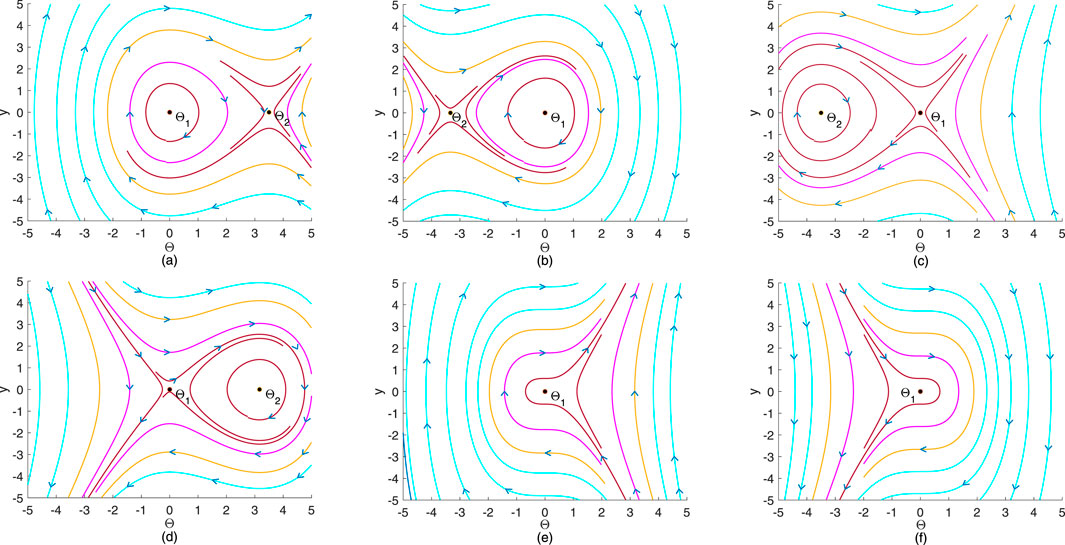
Figure 1. Phase portraits of Equation 2.4. (a) λ₁ = −2.1 and λ₂ = 0.6. (b) λ₁ = −2 and λ₂=0.6. (c) λ₁ = 2.1 and λ₂ = 0.6. (d) Phase portrait with λ₁ = 1.9 and λ₂ = −0.6. (e) Phase portrait with λ₁ = 0 and λ₂ = 2.1. (f) Phase portrait with λ₁ = 0 and λ₂=−1.6.

Multiple attractors and bifurcation phenomena often occur in some nonlinear dynamical systems. Small perturbations can cause the system to shift from one attractor to another, causing the orbit of the system state to become irregular and chaotic. Therefore, we will explore whether Equation 2.4 has chaotic behavior in the case of small external perturbations. In order to simulate the chaotic phenomena in the system, a bounded periodic function can be added to Equation 2.4 as an uncertain perturbation factor. The new equations under the perturbation are described as

$\left\{\begin{array}{c}\frac{d\mathrm{\Theta }}{d\zeta }=y,\hfill \\ \frac{dy}{d\zeta }={\lambda }_2{\mathrm{\Theta }}^2+{\lambda }_1\mathrm{\Theta }+A\sin \varpi \zeta .\hfill \end{array}\right.(2.8)$

It can be found that when periodic perturbations are added, some systems become divergent, even though they were previously bounded, such as when ${\lambda }_1=1.1$ and ${\lambda }_2=-0.6$. Some the phase portraits of Equation 2.8 with bounded phenomenon under the reasonable parameters are shown in Figures 2a–d.

Figure 2

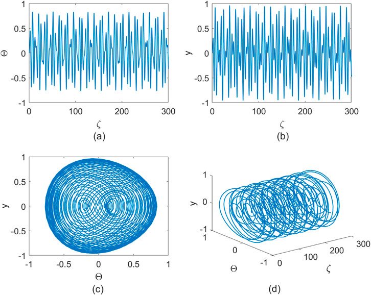
Figure 2. Chaotic behavior of Equation 2.8 at ${\lambda }_1=-2.1,{\lambda }_2=0.6,A=0.5,\varpi =1$. (a) Times series about (θ). (b) Times series about y. (c) 2D phase portrait. (d) 3D trajectory.

3 Traveling wave solutions of Equation 1.2

In this section, some new exact traveling wave solutions of Equation 1.2 are studied based on the theory of the polynomial complete discriminant system [38] and root formula for a cubic polynomial equation. Finally, we demonstrate the solution structure using some two- or three-dimensional pictures.

3.1 Solving procedure

Equation 2.3 is integrated with regard to $\zeta$ once again to obtain

${\left({\mathrm{\Theta }}^{\prime }\right)}^2={\eta }_3{\mathrm{\Theta }}^3+{\eta }_2{\mathrm{\Theta }}^2+{\eta }_1\mathrm{\Theta }+{\eta }_0,(3.1)$

where ${\eta }_3=-\frac{2a}{3bpq},{\eta }_2=\frac{p+q}{bp{q}^2}$ and ${\eta }_1$ and ${\eta }_0$ are arbitrary constants. Let $\omega ={({\eta }_3)}^{\frac{1}{3}}\mathrm{\Theta }$, $m_2={\eta }_2{({\eta }_3)}^{-\frac{2}{3}}$, $m_1={\eta }_1{({\eta }_3)}^{-\frac{1}{3}}$, and $m_0={\eta }_0$. Then, Equation 3.1 can be transformed as

${\left({\omega }^{\prime }\right)}^2={\omega }^3+m_2{\omega }^2+m_1\omega +m_0.(3.2)$

We can obtain the integral form of Equation 3.2 as follows

$\pm {\left({\eta }_3\right)}^{\frac{1}{3}}\left(\zeta -{\zeta }_0\right)=\int \frac{1}{\sqrt{{\omega }^3+m_2{\omega }^2+m_1\omega +m_0}}d\omega ,(3.3)$

where ${\zeta }_0$ is the integration constant. Let $F(\omega )={\omega }^3+m_2{\omega }^2+m_1\omega +m_0$. We can obtain the complete discrimination system of $F(\omega )$ as follows:

$\left\{\begin{array}{c}\mathrm{\Delta }=-27{\left(\frac{2m_2^3}{27}+m_0-\frac{m_1{m}_0}{3}\right)}^2-4{\left(m_1-\frac{m_2^2}{3}\right)}^3\hfill \\ H_1=m_1-\frac{m_2^2}{3}\hfill \end{array}\right..(3.4)$

According to the complete discrimination system (3.4), the solution of Equation 1.2 has the following four situations.

Case 1. $\mathrm{\Delta }=0,H_1<0$. There is $-27{\left(\frac{2m_2^3}{27}+m_0-\frac{m_1{m}_0}{3}\right)}^2=4{\left(m_1-\frac{m_2^2}{3}\right)}^3<0$. Then, $F(\omega )$ has two real roots and a single real root. Using the cubic derivation formula, we obtain

$F\left(\omega \right)={\left(\omega -\upsilon \right)}^2\left(\omega -\mu \right),$

where $\upsilon =-\frac{m_2{m}_1-9m_0}{2(m_2^2-3m_1)},\mu =-m_2+\frac{m_2{m}_1-9m_0}{m_2^2-3m_1}$. Then, the solutions of Equation 3.2 are

$\begin{array}{ll}\hfill & {\mathrm{\Theta }}_1\left(\zeta \right)={\left({\eta }_3\right)}^{-\frac{1}{3}}\left\{\left(m_2-\frac{3\left(m_2{m}_1-9m_0\right)}{2\left(m_2^2-3m_1\right)}\right)\right.\hfill \\ \hfill & \left.\cdot {\tanh }^2\left[\frac{1}{2}{\left(m_2-\frac{3\left(m_2{m}_1-9m_0\right)}{2\left(m_2^2-3m_1\right)}\right)}^{\frac{1}{2}}{\left({\eta }_3\right)}^{\frac{1}{3}}\left(\zeta -{\zeta }_0\right)\right]-m_2+\frac{m_2{m}_1-9m_0}{m_2^2-3m_1}\right\},\hfill \end{array}(3.5)$

$\begin{array}{ll}\hfill & {\mathrm{\Theta }}_2\left(\zeta \right)={\left({\eta }_3\right)}^{-\frac{1}{3}}\left\{\left(m_2-\frac{3\left(m_2{m}_1-9m_0\right)}{2\left(m_2^2-3m_1\right)}\right)\right.\hfill \\ \hfill & \left.\cdot {\coth }^2\left[\frac{1}{2}{\left(m_2-\frac{3\left(m_2{m}_1-9m_0\right)}{2\left(m_2^2-3m_1\right)}\right)}^{\frac{1}{2}}{\left({\eta }_3\right)}^{\frac{1}{3}}\left(\zeta -{\zeta }_0\right)\right]-m_2+\frac{m_2{m}_1-9m_0}{m_2^2-3m_1}\right\},\hfill \end{array}(3.6)$

$\begin{array}{ll}\hfill & {\mathrm{\Theta }}_3\left(\zeta \right)={\left({\eta }_3\right)}^{-\frac{1}{3}}\left\{\left(-m_2+\frac{3\left(m_2{m}_1-9m_0\right)}{2\left(m_2^2-3m_1\right)}\right)\right.\hfill \\ \hfill & \left.\cdot {\tan }^2\left[\frac{1}{2}{\left(-m_2+\frac{3\left(m_2{m}_1-9m_0\right)}{2\left(m_2^2-3m_1\right)}\right)}^{\frac{1}{2}}{\left({\eta }_3\right)}^{\frac{1}{3}}\left(\zeta -{\zeta }_0\right)\right]-m_2+\frac{m_2{m}_1-9m_0}{m_2^2-3m_1}\right\}.\hfill \end{array}(3.7)$

We substitute $\zeta =\frac{p{t}^{\alpha }}{\alpha }+\frac{q{x}^{\beta }}{\beta }$, $m_2={\eta }_2{({\eta }_3)}^{-\frac{2}{3}}$, $m_1={\eta }_1{({\eta }_3)}^{-\frac{1}{3}}$, ${\eta }_3=-\frac{2a}{3bpq}$, and ${\eta }_2=\frac{p+q}{bp{q}^2}$ into Equations 3.5–3.7. Then, the traveling wave solutions of Equation 1.2 are obtained as follows

${\mathrm{\Theta }}_1\left(x,t\right)=-{\left(\frac{3bpq}{2a}\right)}^{\frac{1}{3}}\left\{R_1{\tanh }^2\left[\frac{R_1^{\frac{1}{2}}}{2}{\left(-\frac{2a}{3bpq}\right)}^{\frac{1}{3}}\left(\frac{p{t}^{\alpha }}{\alpha }+\frac{q{x}^{\beta }}{\beta }-{\zeta }_0\right)\right]+R_2\right\},(3.8)$

${\mathrm{\Theta }}_2\left(x,t\right)=-{\left(\frac{3bpq}{2a}\right)}^{\frac{1}{3}}\left\{R_1{\coth }^2\left[\frac{R_1^{\frac{1}{2}}}{2}{\left(\frac{2a}{3bpq}\right)}^{\frac{1}{3}}\left(\frac{p{t}^{\alpha }}{\alpha }+\frac{q{x}^{\beta }}{\beta }-{\zeta }_0\right)\right]+R_2\right\},(3.9)$

${\mathrm{\Theta }}_3\left(x,t\right)=-{\left(\frac{3bpq}{2a}\right)}^{\frac{1}{3}}\left\{-R_1{\tanh }^2\left[\frac{{\left(-R_1\right)}^{\frac{1}{2}}}{2}{\left(-\frac{2a}{3bpq}\right)}^{\frac{1}{3}}\left(\frac{p{t}^{\alpha }}{\alpha }+\frac{q{x}^{\beta }}{\beta }-{\zeta }_0\right)\right]+R_2\right\},(3.10)$

where $R_1=\frac{p+q}{bp{q}^2}{\left(\frac{3bpq}{2a}\right)}^{\frac{2}{3}}-\frac{9(\frac{{\eta }_1(p+q)}{2aq}-3{\eta }_0)}{{(\frac{3bpq}{2a})}^{\frac{1}{3}}\frac{{(p+q)}^2-3{\eta }_1}{abp{q}^3}},R_2=-\frac{p+q}{bp{q}^2}{\left(\frac{3bpq}{2a}\right)}^{\frac{2}{3}}+\frac{3(\frac{{\eta }_1(p+q)}{2aq}-3{\eta }_0)}{{(\frac{3bpq}{2a})}^{\frac{1}{3}}\frac{{(p+q)}^2-3{\eta }_1}{2abp{q}^3}}$.

Case 2. $\mathrm{\Delta }=0,H_1=0$. There is $-27{\left(\frac{2m_2^3}{27}+m_0-\frac{m_1{m}_0}{3}\right)}^2=4{\left(m_1-\frac{m_2^2}{3}\right)}^3$ and $m_1=\frac{m_2^2}{3}$. Therefore, $F(\omega )$ has three same real roots. Due to the cubic derivation formula, there is $F(\omega )={(\omega -\varrho )}^3$, where $\varrho =-\frac{m_2}{3}$. Then, the solutions of Equation 3.2 are

${\mathrm{\Theta }}_4\left(\zeta \right)=4{\left({\eta }_3\right)}^{-\frac{2}{3}}{\left(\zeta -{\zeta }_0\right)}^{-2}-\frac{m_2}{3}.(3.11)$

We substitute $\zeta =\frac{p{t}^{\alpha }}{\alpha }+\frac{q{x}^{\beta }}{\beta }$, $m_2={\eta }_2{({\eta }_3)}^{-\frac{2}{3}}$, and ${\eta }_3=-\frac{2a}{3bpq}$ into Equation 3.11. Then, the traveling wave solution of Equation 1.2 is obtained as follows:

${\mathrm{\Theta }}_4\left(x,t\right)=4{\left(\frac{3bpq}{2a}\right)}^{\frac{2}{3}}{\left(\frac{p{t}^{\alpha }}{\alpha }+\frac{q{x}^{\beta }}{\beta }-{\zeta }_0\right)}^{-2}-\frac{p+q}{{\left(12a^{2}bp{q}^4\right)}^{\frac{1}{3}}}.(3.12)$

Case 3. $\mathrm{\Delta }>0,H_1<0$. There is $-27{\left(\frac{2m_2^3}{27}+m_0-\frac{m_1{m}_0}{3}\right)}^2-4{\left(m_1-\frac{m_2^2}{3}\right)}^3>0$ and $m_1-\frac{m_2^2}{3}<0$. Then, $F(\omega )$ has three real different roots. Because of the cubic derivation formula, we obtain

$F\left(\omega \right)=\left(\omega -\upsilon \right)\left(\omega -\mu \right)\left(\omega -\varrho \right),$

where

$\begin{array}{ll}\hfill & \upsilon =\frac{-m_2-2{\left(m_2^2-3m_1\right)}^{\frac{1}{2}}\cos \frac{\theta }{3}}{3},\hfill \\ \hfill & \mu =\frac{-m_2+{\left(m_2^2-3m_1\right)}^{\frac{1}{2}}\left(\cos \frac{\theta }{3}-3^{\frac{1}{2}}\sin \frac{\theta }{3}\right)}{3},\hfill \\ \hfill & \varrho =\frac{-m_2+{\left(m_2^2-3m_1\right)}^{\frac{1}{2}}\left(\cos \frac{\theta }{3}+3^{\frac{1}{2}}\sin \frac{\theta }{3}\right)}{3},\hfill \\ \hfill & \theta =\arccos \frac{2\left(m_2^2-3m_1\right)-3m_2{m}_1+27m_0}{2{\left(m_2^2-3m_1\right)}^{\frac{2}{3}}}.\hfill \end{array}$

Furthermore, $\upsilon <\mu <\varrho$ as $\theta \in (0,\pi )$.

If $\upsilon <\omega <\varrho$, then the solution of Equation 3.2 is

${\mathrm{\Theta }}_5\left(\zeta \right)={\left({\eta }_3\right)}^{-\frac{1}{3}}\left[\upsilon +\left(\mu -\upsilon \right){\text{sn}}^2\left(\frac{1}{2}{\left(\varrho -\upsilon \right)}^{\frac{1}{2}}{\left({\eta }_3\right)}^{\frac{1}{3}}\left(\zeta -{\zeta }_0\right),m\right)\right],(3.13)$

where $m={\left(\frac{\cos (\frac{\pi }{6}+\frac{\theta }{3})}{\cos (\frac{\pi }{6}-\frac{\theta }{3})}\right)}^{\frac{1}{2}}$ and sn is the Jacobi elliptic sine function. Replacing these variables $\zeta$, $m_2$, $m_1$, ${\eta }_3$, and ${\eta }_2$ by their specific expressions for Equation 3.13, the traveling wave solutions of Equation 1.2 can be obtained as follows:

$\begin{array}{ll}\hfill & {\mathrm{\Theta }}_5\left(x,t\right)=-{\left(\frac{3bpq}{2a}\right)}^{\frac{1}{3}}\left[\frac{-p-q}{{\left(12a^{2}bp{q}^4\right)}^{\frac{1}{3}}}-\frac{2}{3}{R}_1\cos \frac{\theta }{3}\right.+\frac{{}^3\sqrt{3}{R}_1}{3}\cos \left(\frac{\pi +2\theta }{6}\right)\hfill \\ \hfill & \left.\times {\text{sn}}^2\left(-\frac{a^{\frac{1}{3}}{\cos }^{\frac{1}{2}}\left(\frac{\pi -2\theta }{6}\right)}{{\left(12bpq\right)}^{\frac{1}{3}}}\left(\frac{p{t}^{\alpha }}{\alpha }+\frac{q{x}^{\beta }}{\beta }-{\zeta }_0\right),m\right)\right].\hfill \end{array}(3.14)$

If $\omega >\varrho$, then the solution of Equation 3.2 is

${\mathrm{\Theta }}_6\left(\zeta \right)={\left({\eta }_3\right)}^{-\frac{1}{3}}\left[\frac{\varrho -\mu {\text{sn}}^2\left(\frac{1}{2}{\left(\varrho -\upsilon \right)}^{\frac{1}{2}}{\left({\eta }_3\right)}^{\frac{1}{3}}\left(\zeta -{\zeta }_0\right),m\right)}{{\text{cn}}^2\left(\frac{1}{2}{\left(\varrho -\upsilon \right)}^{\frac{1}{2}}{\left({\eta }_3\right)}^{\frac{1}{3}}\left(\zeta -{\zeta }_0\right),m\right)}\right],(3.15)$

where cn is the Jacobi elliptic cosine function. Substituting the specific expression of these variables $\zeta$, $m_2$, $m_1$, ${\eta }_3$, and ${\eta }_2$ into Equation 3.15, the traveling wave solutions of Equation 1.2 can be given as follows

${\mathrm{\Theta }}_6\left(x,t\right)=-{\left(\frac{3bpq}{2a}\right)}^{\frac{1}{3}}\left[\frac{\varrho -\mu {\text{sn}}^2\left(\frac{-a^{\frac{1}{3}}{\cos }^{\frac{1}{2}}\left(\frac{\pi -2\theta }{6}\right)}{{\left(12bpq\right)}^{\frac{1}{3}}}\left(\frac{p{t}^{\alpha }}{\alpha }+\frac{q{x}^{\beta }}{\beta }-{\zeta }_0\right),m\right)}{{\text{cn}}^2\left(\frac{-a^{\frac{1}{3}}{\cos }^{\frac{1}{2}}\left(\frac{\pi -2\theta }{6}\right)}{{\left(12bpq\right)}^{\frac{1}{3}}}\left(\frac{p{t}^{\alpha }}{\alpha }+\frac{q{x}^{\beta }}{\beta }-{\zeta }_0\right),m\right)}\right],(3.16)$

where

$\begin{array}{ll}\hfill & \varrho =\frac{-p-q}{{\left(12a^{2}bp{q}^4\right)}^{\frac{1}{3}}}+\frac{1}{3}{R}_1\cos \left(\frac{\pi -2\theta }{6}\right),\hfill \\ \hfill & \mu =\left(\frac{-p-q}{{\left(12a^{2}bp{q}^4\right)}^{\frac{1}{3}}}+\frac{1}{3}{R}_1\cos \left(\frac{\pi +2\theta }{6}\right)\right),\hfill \\ \hfill & \theta =\arccos \frac{2R_1+\frac{243^{\frac{1}{3}}{\eta }_1\left(p+q\right)}{2aq}+27m_0}{2R_1^{\frac{2}{3}}}.\hfill \end{array}$

Case 4. $\mathrm{\Delta }<0,H_1<0$. There is $-27{\left(\frac{2m_2^3}{27}+m_0-\frac{m_1{m}_0}{3}\right)}^2-4{\left(m_1-\frac{m_2^2}{3}\right)}^3<0$. Then, $F(\omega )$ has only one real root. By applying the cubic derivation formula, we obtain

$F\left(\omega \right)=\left(\omega -\upsilon \right)\left({\omega }^2+\mu \omega +\varrho \right),$

where

$\begin{array}{ll}\hfill & \upsilon =-\frac{1}{3}\left(m_2+Y\right),\mu =\frac{1}{3}\left(-2m_2+Y\right),\varrho =\frac{1}{9}{m}_2^2+\frac{1}{36}\left(\sqrt{3}-4m_2\right)Y^2,\hfill \\ \hfill & Y={}^3\sqrt{m_2^3-9m_2{m}_1+\frac{27}{2}{m}_0+\frac{3}{2}{\left(-3m_2^2{m}_1^2-54m_2{m}_1{m}_0+81m_0^2+12m_2^3{m}_0+12m_1^3\right)}^{\frac{1}{2}}}\hfill \\ \hfill & \hspace{1em}+{}^3\sqrt{m_2^3-9m_2{m}_1+\frac{27}{2}{m}_0-\frac{3}{2}{\left(-3m_2^2{m}_1^2-54m_2{m}_1{m}_0+81m_0^2+12m_2^3{m}_0+12m_1^3\right)}^{\frac{1}{2}}}.\hfill \end{array}$

If $\omega >\upsilon$, then the solution of Equation 3.2 is given as

$\begin{array}{ll}\hfill & {\mathrm{\Theta }}_7\left(\zeta \right)={\left({\eta }_3\right)}^{-\frac{1}{3}}\hfill \\ \hfill & \cdot \left[\upsilon +\frac{2\sqrt{{\upsilon }^2+\upsilon \mu +\varrho }}{1+\text{cn}\left({\left({\upsilon }^2+\upsilon \mu +\varrho \right)}^{\frac{1}{4}}{\left({\eta }_3\right)}^{-\frac{1}{3}}\left(\zeta -{\zeta }_0\right),\frac{1}{2}\left(1-\frac{\alpha +\frac{1}{2}\beta }{{\upsilon }^2+\upsilon \mu +\varrho }\right)\right)}-\sqrt{{\upsilon }^2+\upsilon \mu +\varrho }\right].\hfill \end{array}(3.17)$

Substituting the specific expression of the following variables $\zeta$, $m_2$, $m_1$, ${\eta }_3$, and ${\eta }_2$ into Equation 3.17, the traveling wave solutions of Equation 1.2 can be obtained as follows

$\begin{array}{ll}\hfill & {\mathrm{\Theta }}_7\left(x,t\right)=-{\left(\frac{3bpq}{2a}\right)}^{\frac{1}{3}}\hfill \\ \hfill & \cdot \left[\frac{-p-q}{{\left(36a^{2}bp{q}^4\right)}^{\frac{1}{3}}}-\frac{1}{3}{R}_3+\frac{2\sqrt{R_4}}{1+\text{cn}\left({\left(R_4\right)}^{\frac{1}{4}}-{\left(\frac{3bpq}{2a}\right)}^{\frac{1}{3}}\left(\frac{p{t}^{\alpha }}{\alpha }+\frac{q{x}^{\beta }}{\beta }-{\zeta }_0\right),n\right)}-\sqrt{R_4}\right],\hfill \end{array}(3.18)$

where

$\begin{array}{ll}\hfill & R_3={}^3\sqrt{\frac{9{\left(p+q\right)}^3}{4a^{2}bp{q}^4}+\frac{9{}^3\sqrt{9}{\eta }_1\left(p+q\right)}{2aq}+\frac{27m_0}{2}+\frac{3}{2}W\hspace{0.17em}}\hfill \\ \hfill & +{}^3\sqrt{\frac{9{\left(p+q\right)}^3}{4a^{2}bp{q}^4}+\frac{9{}^3\sqrt{9}{\eta }_1\left(p+q\right)}{2aq}+\frac{27m_0}{2}-\frac{3}{2}W},\hfill \\ \hfill & R_4=\frac{4^{\frac{1}{3}}{\left(p+q\right)}^2}{{\left(9a^4{b}^2{p}^6{q}^2\right)}^{\frac{1}{3}}}+\frac{R_3\left(p+q\right)}{{\left(48a^{2}bp{q}^4\right)}^{\frac{1}{3}}}-\frac{\left(p+q\right)R_3^2}{{\left(324a^{2}bp{q}^4\right)}^{\frac{1}{3}}}+\frac{\sqrt{3}}{36}{R}_3^2,\hfill \\ \hfill & W=\left(-\frac{27{\eta }_1{\left(p+q\right)}^2}{4a^2{q}^2}+\frac{162m_0{\eta }_1\left(p+q\right)}{2aq}+\frac{27m_0{\left(p+q\right)}^3}{a^{2}bp{q}^4}\right.\hfill \\ \hfill & {\left.-\frac{18{\eta }_1^{3}bpq}{2a}+81m_0^2\right)}^{\frac{1}{2}},\hfill \\ \hfill & n=\frac{1}{2}+\frac{\left(p+q\right)}{8{\left(6a^{2}bp{q}^4\right)}^{\frac{1}{3}}{R}_4}+\frac{R_3}{12R_4}.\hfill \end{array}$

3.2 Graphical description

To visualize the structure of these new solutions, the solutions ${\mathrm{\Theta }}_1,{\mathrm{\Theta }}_2$ and ${\mathrm{\Theta }}_3$ are described in the form of two- or three-dimensional pictures (see Figures 3–5). According to the derivation conditions, the appropriate parameters are taken to produce the graphs of the solutions. In each traveling wave solution, there are two fractional derivative parameters, $\alpha$ and $\beta$. We fix $\alpha =0.5$ and observe the effect of $\beta$ on the shapes of the solutions. As observed from these comparison graphs, the smaller the value of $\beta$, the more curved the shape of the solutions.

Figure 3

Figure 3. Figures of the solutions ${\mathrm{\Theta }}_1$ with a = 2, b = −5, p = 3, q = 4, α = 0.5, η₁ = 10, η₀ = 20, ζ₀ = 20. (a) β = 1. (b) β = 0.5. (c) β = 0.3. (d) Change in θ₁ with x when t = 2.6174.

Figure 4

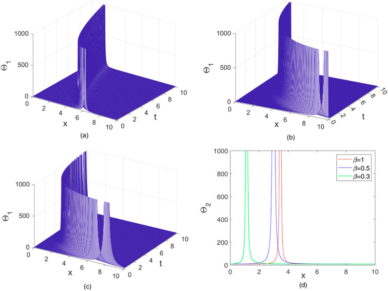
Figure 4. Figures of the solutions ${\mathrm{\Theta }}_2$ with a = 5, b = −5, p = 3, q = 4, α = 0.5, η₁ = 10, η₀ = 11, ζ₀ = 25. (a) β = 1. (b) β = 0.5. (c) β = 0.3. (d) Change in θ₂ with x when t = 3.4673.

Figure 5

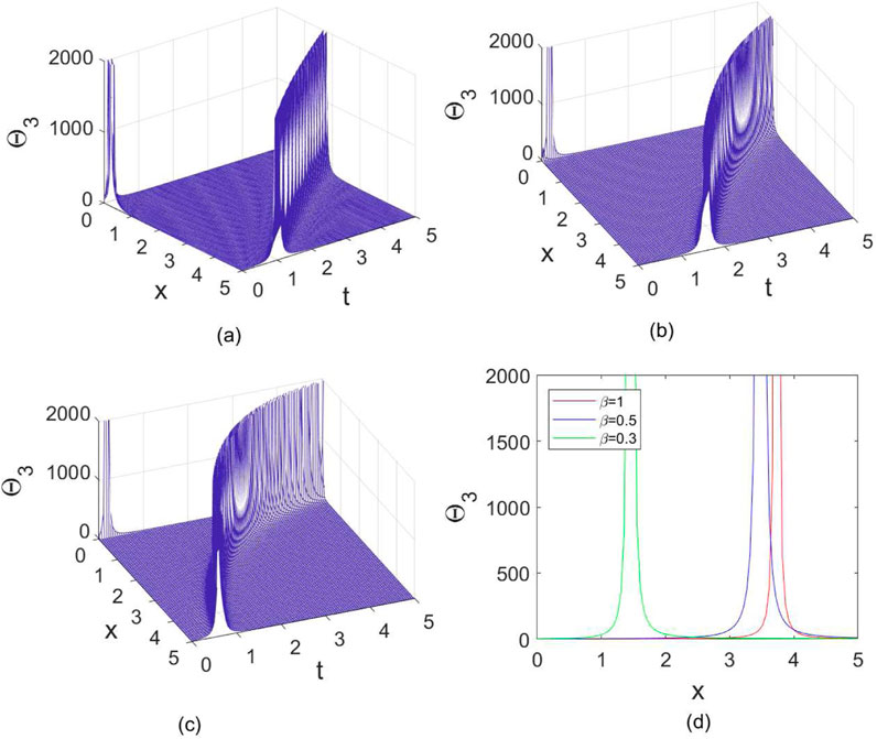
Figure 5. Figures of the solutions ${\mathrm{\Theta }}_3$ with a = 6, b = −5, p = 3, q = 3, α = 0.8, η₁ = 7, η₀ = 1, ζ₀ = −8. (a) β = 1. (b) β = 0.5. (c) β = 0.3. (d) Change in θ₃ with x when t = 2.4121.

4 Conclusion

This paper analyzes the dynamical behavior of the space–time fractional ZKBBM equation and presents seven types of new exact traveling wave solutions by utilizing the theory of the cubic polynomial complete discriminant system and root formulas. These new solutions, including rational, trigonometric, hyperbolic, and Jacobi elliptic function solutions, can be directly applied to simulation, prediction, and control in practical scenarios. Finally, the phase portraits and some of the solutions are plotted using MATLAB software. From these figures, we can clearly and intuitively understand the properties of the equation and the shapes of its solutions under different conditions.

Data availability statement

The original contributions presented in the study are included in the article/supplementary material; further inquiries can be directed to the corresponding author.

Author contributions

SZ: Writing – original draft. ZL: Writing – review and editing.

Funding

The author(s) declare that no financial support was received for the research and/or publication of this article.

Conflict of interest

The authors declare that the research was conducted in the absence of any commercial or financial relationships that could be construed as a potential conflict of interest.

Generative AI statement

The author(s) declare that no Generative AI was used in the creation of this manuscript.

Publisher’s note

All claims expressed in this article are solely those of the authors and do not necessarily represent those of their affiliated organizations, or those of the publisher, the editors and the reviewers. Any product that may be evaluated in this article, or claim that may be made by its manufacturer, is not guaranteed or endorsed by the publisher.

References

1. Zabusky NJ, Kruskal MD. Interaction of “solitons” in a collisionless plasma and the recurrence of initial states. Phys Rev Lett (1965) 15(6):240–3. doi:10.1103/physrevlett.15.240

CrossRef Full Text | Google Scholar

2. Khan AM, Gaur S, Suthar DL. Predicting the solution of fractional order differential equations with Artificial Neural Network. Partial Differential Equations Appl Maths (2024) 10:100690. doi:10.1016/j.padiff.2024.100690

CrossRef Full Text | Google Scholar

3. Deogan AS, Dilz R, Caratelli D. On the application of fractional derivative operator theory to the electromagnetic modeling of frequency dispersive media. Mathematics (2024) 12(7):932. doi:10.3390/math12070932

CrossRef Full Text | Google Scholar

4. Megahid SF, Abouelregal AE, Sedighi HM. Modified Moore-Gibson-Thompson Pennes’ bioheat transfer model for a finite biological tissue subjected to harmonic thermal loading. Mech Time-depend Mater (2024) 28:1441–63. doi:10.1007/s11043-023-09647-3

CrossRef Full Text | Google Scholar

5. Wang N, Xing G, Zhu T, Zhou H, Shi Y. Propagating seismic waves in VTI attenuating media using fractional viscoelastic wave equation. J Geophys Res Solid Earth (2022) 127:e2021JB023280. doi:10.1029/2021jb023280

CrossRef Full Text | Google Scholar

6. Li Y, Zhou Z, Zhang N. Fractional derivative method for anomalous aquitard flow in a leaky aquifer system with depth-decaying aquitard hydraulic conductivity. Water Res (2024) 249:120957. doi:10.1016/j.watres.2023.120957

PubMed Abstract | CrossRef Full Text | Google Scholar

7. Fan E, Zhang J. Applications of the Jacobi elliptic function method to special-type nonlinear equations. Phys Lett A (2002) 305:383–92. doi:10.1016/s0375-9601(02)01516-5

CrossRef Full Text | Google Scholar

8. Yan ZL. Abundant families of Jacobi elliptic function solutions of the (2+1)-dimensional integrable Davey–Stewartson-type equation via a new method. Chaos Solitons Fractals (2003) 18:299–309. doi:10.1016/s0960-0779(02)00653-7

CrossRef Full Text | Google Scholar

9. Yan C. A simple transformation for nonlinear waves. Phys Lett A (1996) 224:77–84. doi:10.1016/s0375-9601(96)00770-0

CrossRef Full Text | Google Scholar

10. Wazwaz AM. A sine-cosine method for handling nonlinear wave equations. Math Comput Model (2004) 40:499–508. doi:10.1016/j.mcm.2003.12.010

CrossRef Full Text | Google Scholar

11. Wang M, Li X, Zhang J. The (G′, G)-expansion method and travelling wave solutions of nonlinear evolution equations in mathematical physics. Phys Lett A (2008) 372:417–23. doi:10.1016/j.physleta.2007.07.051

CrossRef Full Text | Google Scholar

12. Zhang H. New application of the (G′, G)-expansion method. Commun Nonlinear Sci Numer Simulation (2009) 14:3220–5. doi:10.1016/j.cnsns.2009.01.006

CrossRef Full Text | Google Scholar

13. Zaman UH, Arefin MA, Akbar MA, Uddin MH. Analyzing numerous travelling wave behavior to the fractional-order nonlinear Phi-4 and Allen-Cahn equations throughout a novel technique. Results Phys (2022) 37:105486. doi:10.1016/j.rinp.2022.105486

CrossRef Full Text | Google Scholar

14. Uddin MH, Zaman UH, Arefin MA, Akbar MA. Nonlinear dispersive wave propagation pattern in optical fiber system. Chaos Solitons Fractals (2022) 164:112596. doi:10.1016/j.chaos.2022.112596

CrossRef Full Text | Google Scholar

15. Harun-Or-Roshid MdAzizur Rahman. The e^−ϕ(η)-expansion method with application in the (1+1)-dimensional classical Boussinesq equations. Results Phys (2014) 4:150–5. doi:10.1016/j.rinp.2014.07.006

CrossRef Full Text | Google Scholar

16. Filiz A, Ekici M. Sonmezoglu A. F-expansion method and new exact solutions of the Schrödinger-KdV equation. Scientific World J (2014) 14.

Google Scholar

17. Yang XF, Deng ZC, Wei Y. A Riccati-Bernoulli sub-ODE method for nonlinear partial differential equations and its application. Adv Difference equations (2015) 1:117–33. doi:10.1186/s13662-015-0452-4

CrossRef Full Text | Google Scholar

18. Zafar A, Raheel M, Zafar MQ, Nisar KS, Osman MS, Mohamed RN, et al. Dynamics of different nonlinearities to the perturbed nonlinear schrödinger equation via solitary wave solutions with numerical simulation. Fractal and Fractional (2021) 5(4):213. doi:10.3390/fractalfract5040213

CrossRef Full Text | Google Scholar

19. Islam MT, Aktar MA, Gómez-Aguilar JF, Torres-Jiménez J. Further innovative optical solitons of fractional nonlinear quadratic-cubic Schrödinger equation via two techniques. Opt Quan Electron (2021) 53:1–9. doi:10.1007/s11082-021-03223-0

CrossRef Full Text | Google Scholar

20. Rani M, Ahmed N, Dragomir SS, Mohyud-Din ST, Khan I, Nisar KS. Some newly explored exact solitary wave solutions to nonlinear inhomogeneous Murnaghan’s rod equation of fractional order. J Taibah Univ Sci (2021) 15(1):97–110. doi:10.1080/16583655.2020.1841472

CrossRef Full Text | Google Scholar

21. Islam MT, Akter MA, Gómez-Aguilar JF, Akbar MA. Novel and diverse soliton constructions for nonlinear space-time fractional modified Camassa-Holm equation and Schrodinger equation. Opt Quan Electron (2022) 54(4):227. doi:10.1007/s11082-022-03602-1

CrossRef Full Text | Google Scholar

22. Li Z, Lyu J, Hussain E. Bifurcation, chaotic behaviors and solitary wave solutions for the fractional Twin-Core couplers with Kerr law non-linearity. Scientific Rep (2024) 14:22616. doi:10.1038/s41598-024-74044-w

PubMed Abstract | CrossRef Full Text | Google Scholar

23. Li Z, Zhao S. Bifurcation, chaotic behavior and solitary wave solutions for the Akbota equation. AIMS Maths (2024) 9:22590–601. doi:10.3934/math.20241100

CrossRef Full Text | Google Scholar

24. Ma WX. Matrix integrable fourth-order nonlinear schrödinger equations and their exact soliton solutions. Chin Phys Lett (2022) 39(10):100201. doi:10.1088/0256-307x/39/10/100201

CrossRef Full Text | Google Scholar

25. Ma WX. Matrix integrable fifth-order mKdV equations and their soliton solutions. Chin Phys B (2023) 32(2):020201. doi:10.1088/1674-1056/ac7dc1

CrossRef Full Text | Google Scholar

26. Ma WX. Sasa-Satsuma type matrix integrable hierarchies and their Riemann-Hilbert problems and soliton solutions. Physica D (2023) 446:133672. doi:10.1016/j.physd.2023.133672

CrossRef Full Text | Google Scholar

27. Li C, N’Gbo N’G, Su F. Finite difference methods for nonlinear fractional differential equation with ψ-Caputo derivative. Physica D (2024) 460:134103. doi:10.1016/j.physd.2024.134103

CrossRef Full Text | Google Scholar

28. Hanif M, Habib MA. Exact solitary wave solutions for a system of some nonlinear space-time fractional differential equations. Pramana-j Phys (2020) 94(1):7. doi:10.1007/s12043-019-1864-6

CrossRef Full Text | Google Scholar

29. Shakeel M, Tauseef Mohyud-Din S. New (G′/G)-expansion method and its application to the Zakharov-Kuznetsov CBenjamin-Bona-Mahony (ZKCBBM) equation. J Assoc Arab Universities Basic Appl Sci (2015) 18:66–81. doi:10.1016/j.jaubas.2014.02.007

CrossRef Full Text | Google Scholar

30. Ali A, Iqbal MA, Mohyud-Din ST. Solitary wave solutions Zakharov-Kuznetsov-Benjamin-Bona-Mahony (ZK-BBM) equation. J Egypt Math Soc (2016) 24:44–8. doi:10.1016/j.joems.2014.10.008

CrossRef Full Text | Google Scholar

31. Ali A, Iqbal MA, Tauseef Mohyud-Din S. Traveling wave solutions of generalized Zakharov-Kuznetsov-Benjamin-Bona-Mahony and simplified modified form of Camassa-Holm equation exp(−ϕ(η))-Expansion method. Egypt J Basic Appl Sci (2016) 3:134–40. doi:10.1016/j.ejbas.2016.01.001

CrossRef Full Text | Google Scholar

32. Seadawy AR, Lu D, Khater MMA. Solitary wave solutions for the generalized Zakharov-Kuznetsov-Benjamin-Bona-Mahony nonlinear evolution. J Ocean Eng Sci (2017) 2:137–42. doi:10.1016/j.joes.2017.05.002

CrossRef Full Text | Google Scholar

33. Salamat N, Arif AH, Mustahsan M, Missen MMS, Surya Prasath VB. On compacton traveling wave solutions of Zakharov-Kuznetsov-Benjamin-Bona-Mahony (ZK-BBM) equation. Comput Appl Maths (2022) 41:365. doi:10.1007/s40314-022-02082-z

CrossRef Full Text | Google Scholar

34. Mehmet Baskonus H, Gao W. Investigation of optical solitons to the nonlinear complex Kundu-Eckhaus and Zakharov-Kuznetsov-Benjamin-Bona-Mahony equations in conformable. Opt Quan Electron (2022) 54:388. doi:10.1007/s11082-022-03774-w

PubMed Abstract | CrossRef Full Text | Google Scholar

35. Zaman UHM, Asif Arefin M, Ali Akbar M, Hafiz Uddin M. Stable and effective traveling wave solutions to the non-linear fractional Gardner and Zakharov-Kuznetsov-Benjamin-Bona-Mahony equations. Partial Differential Equations Appl Maths (2023) 7:100509. doi:10.1016/j.padiff.2023.100509

CrossRef Full Text | Google Scholar

36. Alizadeh F, Hincal E, Hosseini K, Hashemi MS, Das A. The $$(2 + 1)$$-dimensional generalized time-fractional Zakharov Kuznetsov Benjamin Bona Mahony equation: its classical and nonclassical symmetries, exact solutions, and conservation laws. Opt Quan Electron (2023) 55:1061. doi:10.1007/s11082-023-05387-3

CrossRef Full Text | Google Scholar

37. Jibin L, Huihui D. On the study of singular nonlinear traveling wave equations: dynamical system approach. Beijing: Science Press (2007).

Google Scholar

38. Liu C. Applications of complete discrimination system for polynomial for classifications of traveling wave solutions to nonlinear differential equations. Comput Phys Commun (2010) 181:317–24. doi:10.1016/j.cpc.2009.10.006

CrossRef Full Text | Google Scholar

39. Shan Z, Li Z. The analysis of traveling wave solutions and dynamical behavior for the stochastic coupled Maccari’s system via Brownian motion. Ain Shams Eng J (2024) 15:103037. doi:10.1016/j.asej.2024.103037

CrossRef Full Text | Google Scholar

40. Shan Z. Chaos analysis and traveling wave solutions for fractional (3+1)-dimensional Wazwaz Kaur Boussinesq equation with beta derivative. Scientific Rep (2024) 14:23034. doi:10.1038/s41598-024-74606-y

CrossRef Full Text | Google Scholar

41. Khalil R, Al HM, Yousef A, Sababheh M. A new definition of fractional derivative. J Comput Appl Maths (2014) 264:65–70. doi:10.1016/j.cam.2014.01.002

CrossRef Full Text | Google Scholar