Estimating contagion dynamics models on networks via data assimilation

Network-based contagion models are widely used to describe the spread of epidemics, computer viruses and opinions, yet estimating their states, parameters and hyperparameters remains challenging, especially when only macro-level data are available. We therefore aimed to develop a data-assimilation framework capable of performing this estimation without requiring node-level observations. An ensemble Kalman filter-based approach was designed to assimilate macroscopic data into network-based Susceptible–Infected–Recovered models with heterogeneous parameters. The method was evaluated under three scenarios: (i) homogeneous parameters with known network topology; (ii) heterogeneous parameters with known topology; and (iii) homogeneous parameters with unknown topology. Across all tested scenarios, the proposed algorithms accurately estimated both the system states and the underlying parameter/hyperparameter when the network size are sufficiently large, demonstrating scalability and robustness even when only aggregate statistics were available. The results indicate that the proposed assimilation framework can reliably estimate network-based contagion dynamics from macro-level observations, obviating the need for costly node-level monitoring and offering a practical tool for real-time epidemic analysis and forecasting.

1 Introduction

In contagion dynamics [4], nodes on a network are in one of several states at any given moment, and the transition of a node’s state depends on its own state or the states of its neighboring nodes. The spread of epidemics, computer viruses, and public opinion over networks can all be characterized and studied using the principles of contagion dynamics. This has led to the emergence of fields such as epidemic dynamics [14], cybersecurity dynamics [20], and opinion dynamics [18]. Owing to the similarities in the underlying mechanisms of these fields, models from one domain are often used to study others and can be enhanced in the process. A prime example is the “compartmental models” in epidemic dynamics, such as the susceptible–infected–susceptible (SIS) and susceptible–infected–recovered (SIR) models [3], which have been adapted to study cybersecurity dynamics with the incorporation of considerations for network topology [22, 25].

Although a variety of models and corresponding theories, such as the epidemic threshold theory associated with the SIS model [1], have been proposed, contagion dynamics and its derived fields still face many pressing issues. The most important of these is the uncertainty of model parameters, a problem that has been raised in both epidemic dynamics [14] and cybersecurity dynamics [21]. Nearly all studies are based on the core assumption that model parameters, such as infection rates of viruses, recovery rates of disease, and the intensity of cyber-attacks and network structures, are known. For example, the epidemic threshold is entirely determined by model parameters [1], and the dynamical evolution of some models is also completely determined by these parameters [22, 25]. Without knowing the model parameters, all these works will remain at the theoretical level and cannot be verified for correctness or used to solve practical problems, contradicting the original intention of establishing these fields.

However, the reality is that these parameters are difficult to obtain. For example, the infection and recovery rates of viruses and computer viruses cannot be directly measured, and network structures often contain substantial erroneous information [12]. Therefore, how to extract model parameters from available data has become an emerging direction [14, 21].

Current work on parameter estimation in contagion dynamics is largely based on traditional contagion models, which assume that (i) connections between nodes are well mixed, and thus, the models do not account for the effects of network topology; and (ii) parameters between nodes are homogeneous [17, 23]. However, Newman pointed out that these two assumptions are not realistic: the number of people each node can come into contact with varies greatly, and the ability of different infectors to infect others is also different [11]. Therefore, it is necessary to incorporate network topology into consideration. In the current work on parameter estimation in network-based contagion dynamics, the data are at the node level—that is, the information of each node over time is required [15]. However, such data are often difficult to obtain in reality. To the best of our knowledge, there are currently no works on estimating parameters of network-based contagion dynamics models with heterogeneous parameters from macroscopic data like the average infection rate.

Data assimilation (DA) is a technique that integrates observational data with numerical models to optimize the state and parameters of the model, thereby bringing it closer to the behavior of the real system. In practical applications, data assimilation methods are used not only to improve the initial state of the model but also to estimate key parameters within the model. For example, in meteorology, by assimilating observational data from ground stations and satellites, parameters such as temperature, humidity, and wind fields in atmospheric models can be estimated, thereby enhancing the accuracy of weather forecasts [8]. By dynamically adjusting model parameters to fit observational data, data assimilation significantly enhances the predictive capabilities of models and the understanding of complex systems.

To address the problem of extracting parameters from available data for contagion dynamics models, we propose a method based on the integration of contagion dynamics models and data assimilation. This method not only estimates model parameters but also aids in predicting the state of dynamics. Our contributions are highlighted as follows:

• We proposed a new algorithm that can assimilate macro-data and estimate the parameters of the underlying network-based dynamical model with heterogeneous parameters, which not only fills the gap in the literature but also strengthens the connection between contagion dynamics theoretical models and practical applications.

• In the absence of real-world data, we validated the effectiveness of the proposed algorithm using toy models and investigated its performance under node-heterogeneous parameters and unknown network topology; these results suggest that even when the information on the network topology is uncertain, relatively accurate parameter estimation is still achievable if certain statistical properties of the network are known.

The remainder of this article is organized as follows: Section 2 lists the related work. Section 3 interprets the models and our method. Section 4 conducts the numerical analysis. Finally, Section 5 concludes the paper. There are many abbreviations of proper nouns in the text. For the reader’s convenience, the abbreviations and their corresponding full names are listed in Table 1.

Table 1

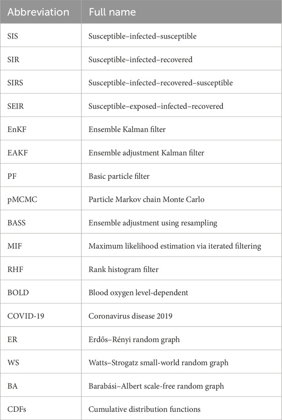
Table 1. Abbreviations and their full names.

2 Related works

There are some studies that utilize data assimilation algorithms to predict the model’s states and estimate parameters.

[17] proposed a framework based on the ensemble adjustment Kalman filter (EAKF) and the susceptible–infected–recovered–susceptible (SIRS) model for real-time prediction of seasonal influenza outbreaks. The study leveraged real-time estimates of influenza infection rates provided by Google Flu Trends, assimilating these data into the SIRS model via the EAKF to optimize the model’s state variables and parameter estimates. The technical strength of the EAKF lies in its ability to dynamically adjust model parameters and state variables, aligning them with actual observational data and enabling the estimation of key epidemiological parameters, such as the average infectious period (D) and the basic reproductive number $R_{0,\max }$, through the data assimilation process. These parameter estimations not only enhance the model’s capacity to fit the dynamics of influenza transmission but also strengthen its ability to predict future influenza activity.

[23] compared the performances of six advanced filtering methods in influenza epidemic modeling and forecasting. The six filtering methods include three types of particle filters, namely, basic particle filter (PF), maximum likelihood estimation via iterated filtering (MIF), and particle Markov chain Monte Carlo (pMCMC), and three types of ensemble filters, namely, ensemble Kalman filter (EnKF), EAKF, and rank histogram filter (RHF). The study used a humidity-driven SIRS model and utilized influenza incidence data from 115 U.S. cities for simulation and retrospective forecasting. The results indicate that the basic particle filter and EnKF methods perform better in fitting historical influenza data and estimating parameters.

[9] proposed an improved state filter algorithm for SIR epidemic forecasting, known as ensemble adjustment using resampling (BASS), which aims to enhance the performance of epidemic predictions based on the SIR model by integrating the linear correction of the EnKF with the resampling technique of the PF. BASS corrects the state variables using maximum likelihood estimation and updates the ensemble by sampling from the best-performing particles, thereby optimizing the state variables and parameter estimates of the model. Empirical results demonstrate that BASS achieves the lowest root-mean-square error and the highest correlation coefficient in 11 of 14 real-world scenarios.

[5] presented an extended susceptible–exposed–infected–recovered (SEIR) model with a vaccination compartment to simulate and forecast the COVID-19 pandemic in Saudi Arabia. The model included seven stages of infection: susceptible, exposed, infectious, quarantined, recovered, dead, and vaccinated. To address uncertainties in the model and improve forecasting skills, the authors used a data assimilation method using the ensemble Kalman filter to estimate model states and parameters by assimilating daily COVID-19 data.

[24] proposed a method based on the hierarchical data assimilation framework to estimate the hyperparameters of spiking neuronal network models for simulating and predicting brain activity. The study considered the role of network topology in the model while also allowing the model’s parameters to be heterogeneous across nodes. It combined hierarchical Bayesian estimation with data assimilation techniques to estimate the distribution of parameters in the mesoscopic neuronal network model using macroscopic blood oxygen level-dependent (BOLD) signal data, rather than directly estimating the exact values of each parameter. Through simulation experiments, the hierarchical data assimilation framework demonstrated high efficiency and accuracy in estimating hyperparameters and simulating BOLD signals while avoiding overfitting.

The aforementioned studies can be summarized as follows: in the field of classical epidemic dynamics, most studies that utilize data assimilation techniques to predict state estimation parameters use models based on the assumptions of homogeneous mixing and homogeneous nodes, without considering the impact of network topology and node heterogeneity on the model. In the field of neuroscience, Zhang et al. challenged these two assumptions and proposed a framework, hierarchical data assimilation, for estimating distribution hyperparameters. However, in their estimation process, the network structure is assumed to be known.

Table 2 presents comparisons between previous studies and our work. In the “Network topology” column, “Fully mixed” indicates that the model does not account for network topology; this will be elaborated upon in the model selection section.

Table 2

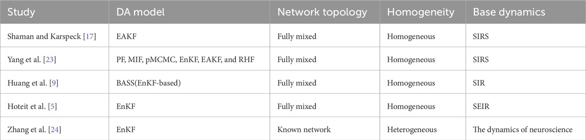
Table 2. Comparison of data assimilation models, network structure assumptions, and node homogeneity assumptions across different studies.

3 Models and methods

3.1 Contagion dynamics

Some classical contagion dynamics models are repeatedly used and investigated across various fields, such as SIS and SEIR [7]. Because the SIR model is the most renowned and extensively studied model in classical epidemiology and is highly representative—with other models such as SIRS and SEIR, mentioned in the Related work section, being its variants [10]—we choose a network security dynamics model based on the SIR model as our model. It is noteworthy that our algorithm can be adapted to other models. Section 4.7 presents a case where we use our algorithm in the SIS model.

Assume that there are $n$ nodes in the network, each of which can be in one of the following three states:

- susceptible (S): nodes that are not yet infected but can contract the virus;

- infected (I): nodes that are currently infected and can transmit the virus to others; or

- recovered (R): nodes that have recovered from the attack of the virus and are now immune.

The network topology can be represented using a directed graph $G=(V,E)$, where $V=\{\mathrm{1,2},\dots ,n\}$ is the node set and $E\subset V\times V$ is the arc set. Node $u\in V$ is an incoming neighbor of node $v\in V$, and $v$ is an outgoing neighbor of node $u$ if $(u,v)\in E$. The adjacency matrix of $G$ is an $n$-dimensional matrix $A={(a_{u,v})}_{n\times n}$, where $a_{u,v}\in \{\mathrm{0,1}\}$ for $u,v\in V$, and $a_{u,v}=1$ if and only if $(u,v)\in E$.

As emphasized earlier, the original SIR model does not account for network topology and assumes homogeneous parameters across all nodes [9]. We assume that the rate of an infected node successfully infecting a susceptible node is $\beta$, and the rate of an infected node recovering and gaining immunity is $\gamma$. Additionally, at time $t$, the fractions of nodes in the susceptible, infected, and recovered states are $s(t)$, $i(t)$, and $r(t)$, respectively. The evolution of the three states is governed by the discrete master equation (Equation 1):

$\begin{array}{cc}\hfill \frac{ds\left(t\right)}{dt}& =-\beta i\left(t\right)s\left(t\right),\hfill \\ \hfill \frac{di\left(t\right)}{dt}& =\beta i\left(t\right)s\left(t\right)-\gamma i\left(t\right),\hfill \\ \hfill \frac{dr\left(t\right)}{dt}& =\gamma i\left(t\right).\hfill \end{array}(1)$

As mentioned in the Related work section, the original model is far from realistic; therefore, we take the network topology into account and assume that the nodes’ parameters are different.

Let $\xi (t)=[{\xi }_1(t),{\xi }_2(t),\dots ,{\xi }_n(t)]$ denote the states of all nodes at time $t$: for each node $v\in V$, ${\xi }_v(t)\in \{\mathrm{0,1,2}\}$, where ${\xi }_v(t)=0$, 1, and 2 indicate that node $v$ is in the susceptible, infected, and recovered states, respectively, at time $t$. If node $v$ is in the infected state, i.e., ${\xi }_v(t)=1$, then ${\beta }_v$ represents the rate that node $v$ infects its outgoing neighbors, while ${\gamma }_v$ denotes the rate of node $v$ recovering. Let $s_v(t)$, $i_v(t)$, and $r_v(t)$ denote the probabilities that node $v$ is in the susceptible, infected, and recovered states, respectively, at time $t$. Then, the evolution of $s_v(t)$, $i_v(t)$, and $r_v(t)$ follows the master equations taking place on $G$: for $v\in V$,

$\begin{array}{cc}\hfill \frac{d{s}_v\left(t\right)}{dt}& =-\left(1-\prod _{u\in V,u\ne v}\left(1-{\beta }_u{a}_{u,v}{i}_v\left(t\right)\right)\right)s_v\left(t\right),\hfill \\ \hfill \frac{d{i}_v\left(t\right)}{dt}& =\left(1-\prod _{u\in V,u\ne v}\left(1-{\beta }_u{a}_{u,v}{i}_v\left(t\right)\right)\right)s_v\left(t\right)-{\gamma }_v{i}_v\left(t\right),\hfill \\ \hfill \frac{d{r}_v\left(t\right)}{dt}& ={\gamma }_v{i}_v\left(t\right).\hfill \end{array}(2)$

3.2 Algorithm for estimating the parameters of contagion dynamics based on EnKF

The main objective of our algorithm is to assimilate macroscopic observational states and estimate the parameters of the underlying dynamical model, with adjustments made according to different scenarios.

3.2.1 Selection of the data assimilation method

From the Related work section [23], two types of data assimilation algorithms are often used in the inference and forecasting of infectious disease models: PF and ensemble filters (including the EnKF and its derivations).

PF and EnKF are both advanced methods for state estimation in nonlinear dynamic systems. The particle filter is a non-parametric filtering technique based on Monte Carlo methods, which approximates the posterior probability distribution of the system using a set of weighted particles. In contrast, the ensemble Kalman filter is a linear filtering method based on ensemble members to estimate the error covariance, making it suitable for efficient state estimation in high-dimensional systems.

Both of these filtering methods can be applied to our approach, and the procedures are similar. Compared to the PF, the EnKF avoids the issue of particle depletion caused by resampling and offers more flexible computation, making it suitable for data assimilation tasks in epidemic models. We compare the performances of the two filtering methods in Section 4.4.3. We adopt the ensemble Kalman filter as our basic method.

3.2.2 Three application scenarios

Below are three scenarios that need to be considered:

1) Scenario 1: The network $G$ is known, and the model is homogeneous, that is, for $v\in V$, ${\beta }_v=\beta$ and ${\gamma }_v=\gamma$, and we need to estimate $\beta$ and $\gamma$.

2) Scenario 2: The network $G$ is known, and the model is heterogeneous. We assume that the compromise probabilities and the recovery probabilities of each node, ${\beta }_v$ and ${\gamma }_v$ for $v\in V$, are sampled from distributions $D_1({\beta }^{\prime })$ and $D_2({\gamma }^{\prime })$, respectively, and we need to estimate ${\beta }^{\prime }$ and ${\gamma }^{\prime }$.

3) Scenario 3: The network $G$ is sampled from a known distribution, and the model is homogeneous. Then, we need to estimate the constants $\beta$ and $\gamma$.

Scenario 1 is the most basic scenario, which takes into account the network topology but still assumes that the parameters are homogeneous. Scenario 2 considers heterogeneous parameters and demonstrates that when there are a sufficient number of nodes in the network, it is the distribution of these parameters—not the individual node values—that influences the contagion dynamics [11]. Scenario 3 takes into account the possibility that the network information in reality may be erroneous or incomplete [13], and it shows that if one grasps the statistical patterns of the network, it is possible to estimate the parameters without strictly knowing the specific structure of the network topology.

The detailed procedure of the algorithm is introduced in the following section.

3.2.3 Evolution system and state vector

Data assimilation methods require an evolution equation, which is corrected at each time step by observations to bring the variables and parameters of the equation closer to the true situation. The set of variables and parameters that need to be updated is referred to as the state vector of the evolution equation. Assume that the state vector is $q$-dimensional and the observations are $r$-dimensional. Let the state vector at time $t_k$ be $x(t_k)\in {\mathbb{R}}^q$. The evolution system generates the state vector $x(t_{k+1})$ and the predicted observation $y(t_{k+1})$ vector for the next moment $t_{k+1}$:

$\begin{array}{cc}\hfill x\left(t_{k+1}\right)& =F\left(x\left(t_k\right),t_k,t_{k+1},w_k\right),\hfill \\ \hfill y\left(t_{k+1}\right)& =H\left(x\left(t_{k+1}\right)\right)+{\eta }_k,\hfill \end{array}$

where $F(\cdot )\in C^1({\mathbb{R}}^q,{\mathbb{R}}^q)$ is the evolution function, $H(\cdot )\in C^1({\mathbb{R}}^q,{\mathbb{R}}^r)$ is the observation function, which extracts the predicted observations $y(t_{k+1})$ from the state vector $x(t_{k+1})$, and the $q$-dimensional Gaussian noise $w_k\sim \mathcal{N}(0,Q_k)$ and the $r$-dimensional Gaussian noise ${\eta }_k\sim \mathcal{N}(0,R_k)$ represent the system noise and the observation noise, where $Q_k$ and $R_k$ are covariance matrices of dimensions $q$ and $r$, respectively.

We define the system state at time $t_k$ as $x(t_k)=\{\bar{i}(t_k),\bar{r}(t_k),{\theta }_1(t_k),{\theta }_2(t_k)\}$, and ${\theta }_1(t_k)$ and ${\theta }_2(t_k)$ correspond to the system parameters at time $t_k$, the meaning of which varies depending on the scenario.

It is worth noting that the evolution system does not directly act on the state variable $x(t_k)$. To reflect the evolution process of Equation 2, we introduce an auxiliary state variable $\xi (t_k)=\{{\xi }_1(t_k),\dots ,{\xi }_n(t_k)\}$ for $x(t_k)$, which represents the state of each node in the network at time $t_k$. At time $t_1$, $\xi (t_1)=({\xi }_1(t_1),\dots ,{\xi }_n(t_1))$ is randomly generated such that $\frac{1}{n}{\displaystyle {\sum }_{v\in V}}\hspace{0.17em}{\mathbf{1}}_{{\xi }_v(t_1)=1}=\bar{i}(t_1)$ and $\frac{1}{n}{\displaystyle {\sum }_{v\in V}}\hspace{0.17em}{\mathbf{1}}_{{\xi }_v(t_1)=2}=\bar{r}(t_1)$. ${\mathbf{1}}_{\cdot }$ is the indicator function. The evolution system is actually the evolution from $\xi (t_k)$ to $\xi (t_{k+1})$, as shown in Equation 3:

$\xi \left(t_{k+1}\right)=f\left(\xi \left(t_k\right),{\theta }_1\left(t_k\right),{\theta }_2\left(t_k\right),t_k,t_{k+1},G\right),(3)$

where $G$ is the network, and let $\bar{i}(t_{k+1})=\frac{1}{n}{\displaystyle {\sum }_{v\in V}}\hspace{0.17em}{\mathbf{1}}_{{\xi }_v(t_k)=1}$ and $\bar{r}(t_{k+1})=\frac{1}{n}{\displaystyle {\sum }_{v\in V}}\hspace{0.17em}{\mathbf{1}}_{{\xi }_v(t_k)=2}$. Then, an evolution from $x(t_k)$ to $x(t_{k+1})$ is completed.

In system $f(\cdot )$, ${\theta }_1(t_k)$ and ${\theta }_2(t_k)$ determine the parameters for each node. In scenarios 1 and 3, for $v\in V$, the infection rate and recovery rate at time $t_{k+1}$ are ${\beta }_v(t_{k+1})=g^{-1}({\theta }_1(t_k))$ and ${\gamma }_v(t_{k+1})=g^{-1}({\theta }_2(t_k))$, respectively, where $g(\cdot )=\frac{\tan (\cdot -\frac{1}{2})\pi }{c}$. This is done because in the subsequent update process, the values of ${\theta }_1$ and ${\theta }_2$ cannot be controlled. By using $g^{-1}(\cdot )$, numbers on the real line can be mapped to the interval (0,1), which is the typical range for $\beta$ and $\gamma$. In addition, the value of $c$ controls the slope of the mapping. After experimentation, it is set to 300.

In Scenario 2, we use the method of “Sampling parameters from the hyperparameter” [24] to update each node’s infection rate and recovery rate. Suppose that ${\mathcal{F}}_{1,{\beta }^{\prime }}(\cdot )$ and ${\mathcal{F}}_{2,{\gamma }^{\prime }}(\cdot )$ are cumulative density functions of the distributions $D_1({\beta }^{\prime })$ and $D_2({\gamma }^{\prime })$, respectively. Then, for $v\in V$,

$\begin{array}{cc}\hfill {\beta }_v\left(t_{k+1}\right)& ={\mathcal{F}}_{1,g^{-1}\left({\theta }_1\left(t_k\right)\right)}^{-1}\left({\mathcal{F}}_{1,g^{-1}\left({\theta }_1\left(t_{k-1}\right)\right)}\left({\beta }_v\left(t_k\right)\right)\right),\hfill \\ \hfill {\gamma }_v\left(t_{k+1}\right)& ={\mathcal{F}}_{1,g^{-1}\left({\theta }_2\left(t_k\right)\right)}^{-1}\left({\mathcal{F}}_{1,g^{-1}\left({\theta }_2\left(t_{k-1}\right)\right)}\left({\gamma }_v\left(t_k\right)\right)\right),\hfill \end{array}$

where $g^{-1}$ is used for the same reason and ${\mathcal{F}}_{1,\cdot }^{-1}$ and ${\mathcal{F}}_{2,\cdot }^{-1}$ are the inverse functions of ${\mathcal{F}}_{1,\cdot }$ and ${\mathcal{F}}_{2,\cdot }$, respectively.

The states and parameters we aim to assimilate are those of the System defined in Equation 2. However, the variables of the System in Equation 2 are the probabilities of each node being in one of the three states, which are the continuous values. Moreover, ${\xi }_v(t)\in \{\mathrm{0,1,2}\}$ is the discrete variable. Therefore, we cannot directly apply the System (Equation 2) as the evolution process $f$. To bridge this gap, we explored various implementations of $f$.

3.2.4 Instantiation of the evolution system

3.2.4.1 Discrete simulation

First, the System (Equation 2) can be discretized, and then the infection process within each time interval can be simulated. Under this condition, $t_k$ is an integer, and then, the evolution of $\xi (t_k)$ follows the discrete-time stochastic dynamics system (Equation 4) taking place on $G$: for $v\in V$ and $k\in \mathbb{N}$,

$\begin{array}{cc}\hfill P\left({\xi }_v\left(t_k+1\right)=1\mid {\xi }_v\left(t_k\right)=0\right)& =1-\prod _{u\in V}\left(1-{\beta }_u{a}_{u,v}{\mathbf{1}}_{\left\{{\xi }_u\left(t_k\right)=1\right\}}\right),\hfill \\ \hfill P\left({\xi }_v\left(t_k+1\right)=2\mid {\xi }_v\left(t_k\right)=1\right)& ={\gamma }_v.\hfill \end{array}(4)$

Specifically, in the simulation, we select a random number $b$ from the uniform distribution $U([\mathrm{0,1}])$, i.e., over the interval [0,1]. If ${\xi }_v(t_k)=0$, then

${\xi }_v\left(t_k+1\right)=\left\{\begin{array}{cc}1\hfill & \text{if\hspace{0.17em}}b<P\left({\xi }_v\left(t_k+1\right)=1\mid {\xi }_v\left(t_k\right)=0\right),\hfill \\ 0\hfill & \text{otherwise}.\hfill \end{array}\right.$

Similarly, if ${\xi }_v(t_k)=1$, then

${\xi }_v\left(t_k+1\right)=\left\{\begin{array}{cc}2\hfill & \text{if\hspace{0.17em}}b<P\left({\xi }_v\left(t_k+1\right)=2\mid {\xi }_v\left(t_k\right)=1\right),\hfill \\ 1\hfill & \text{otherwise}.\hfill \end{array}\right.$

Moreover, the Evolve System (Equation 3) represents the process of continuing the above simulation until the time reaches $t_{k+1}$.

3.2.4.2 Gillespie-based simulation

Second, without considering discretization, the System (Equation 2) can be simulated using the Gillespie algorithm [6, 16]. The Evolve System (Equation 3) for simulating the System (Equation 2) using the Gillespie algorithm over the time interval from $t_k$ to $t_{k+1}$ is shown in Algorithm 1.

Algorithm 1

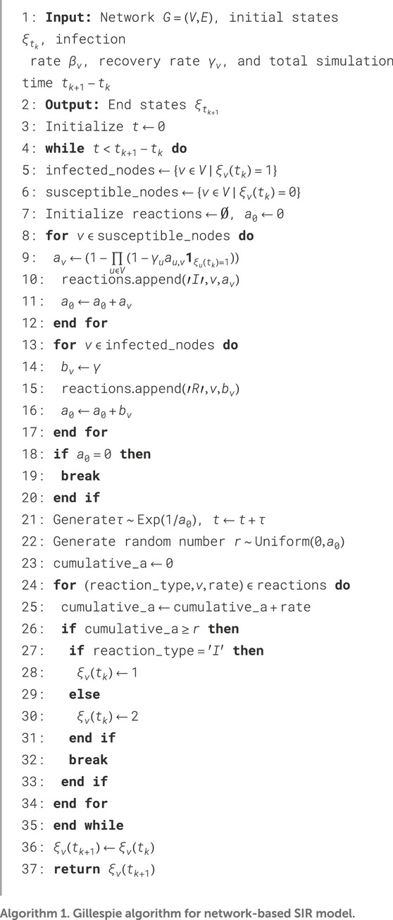
Algorithm 1. Gillespie algorithm for network-based SIR model.

3.2.4.3 Random sampling-based simulation

Third, the Evolve System (Equation 3) can directly evolve the System (Equation 2) and subsequently sample $\xi (t_{k+1})$ based on the probabilities of nodes being in each state. That is,

$s_v\left(t_k\right),i_v\left(t_k\right),r_v\left(t_k\right)=\left\{\begin{array}{cc}\hfill & \mathrm{1,0,0}\text{\hspace{0.17em}if\hspace{0.17em}}{\xi }_v\left(t_k\right)=0,\hfill \\ \hfill & \mathrm{0,1,0}\text{\hspace{0.17em}if\hspace{0.17em}}{\xi }_v\left(t_k\right)=1,\hfill \\ \hfill & \mathrm{0,0,1}\text{\hspace{0.17em}if\hspace{0.17em}}{\xi }_v\left(t_k\right)=2.\hfill \end{array}\right.$

Then, all the triplets $(s_v(t_k),i_v(t_k),r_v(t_k))$ are put into the System (Equation 2) to evolve for $t_{k+1}{t}_k$ time, and the result is denoted as $(s_v(t_{k+1}),i_v(t_{k+1}),r_v(t_{k+1}))$. For $v\in V$, ${\xi }_v(t_{k+1})$ is sampled from $\{\mathrm{0,1,2}\}$ with probabilities $s_v(t_{k+1})$, $i_v(t_{k+1})$, and $r_v(t_{k+1})$.

It should be pointed out that our algorithm is independent of the choice of the System (Equation 3), as long as Equation 3 is a mapping that reflects the discrete-state-to-discrete-state transition of the System (Equation 2). Therefore, our algorithm is applicable to both discrete-time and continuous-time dynamics.

3.2.5 Algorithmic procedure

3.2.5.1 Observation and its generation

The observations are the obtained macroscopic time-series data: assume that during the time interval $[0,T]$, we have sampled $K$ data points ${\{y_{t_k}\}}_{k=1}^K$, where $0\le t_1<t_2<\dots <t_K\le T$. In particular, $y_{t_k}$ represents the average number of infected individuals and the average number of recovered individuals in the system at time $t_k$, i.e.,

$y_{t_k}=\left(\bar{i}\left(t_k\right),\bar{r}\left(t_k\right)\right),$

where $\bar{i}(t_k)=\frac{1}{n}{\displaystyle {\sum }_{v\in V}}\hspace{0.17em}{\mathbf{1}}_{{\xi }_v(t_k)=1}$ and $\bar{r}(t_k)=\frac{1}{n}{\displaystyle {\sum }_{v\in V}}\hspace{0.17em}{\mathbf{1}}_{{\xi }_v(t_k)=2}$.

Due to the lack of real data, we use the Evolve System described in Section 3.2.3 to generate observation data at given time points ${\{t_k\}}_{k=1}^K$.

3.2.5.2 Initialization

We generate $N$ ensemble members, where each ensemble member is a copy of the Evolve System (Equation 3). For simplicity, we denote $\{N\}$ by $\{\mathrm{1,2},\dots ,N\}$. For the $\ell$th ensemble member, we add the subscript $\ell$ to each variable to distinguish it, thereby indicating that the variable belongs to the ensemble member $\ell$.

At the initial time $t_1$, for ensemble members $\ell$, sample ${\bar{i}}_{\ell }^{+}(t_1)$, ${\bar{r}}_{\ell }^{+}(t_1)$, ${\beta }_{\ell }^{+}(t_1)$, and ${\gamma }_{\ell }^{+}(t_1)$ (or ${\beta }_{\ell }^{\prime ,+}(t_1)$ and ${\gamma }_{\ell }^{\prime ,+}(t_1)$) from the initial distribution, and $x_{\ell }^{+}(t_1)=({\bar{i}}_{\ell }^{+}(t_1),{\bar{r}}_{\ell }^{+}(t_1),{\theta }_{1,\ell }^{+}(t_1),{\theta }_{2,\ell }^{+}(t_1))$, where $({\theta }_{1,\ell }^{+}(t_1),{\theta }_{2,\ell }^{+}(t_1))$ is $(g({\beta }_{\ell }^{+}(t_1)),g({\gamma }_{\ell }^{+}(t_1)))$ in scenarios 1 and 3 and $(g({\beta }_{\ell }^{\prime ,+}(t_1)),g({\gamma }_{\ell }^{\prime ,+}(t_1)))$ in Scenario 2.

To distinguish from the components of $\xi (t_k)$, denoted as ${\xi }_v(t_k)$, we use ${\xi }_{,\ell }(t_k)$ to represent the state variables of all nodes belonging to the $\ell$th set member at time step $t_k$. At time $t_1$, ${\xi }_{,\ell }^{+}(t_1)=({\xi }_{1,\ell }^{+}(t_1),\dots ,{\xi }_{n,\ell }^{+}(t_1))$ is randomly generated such that $\frac{1}{n}{\displaystyle \sum _{v\in V}}{\mathbf{1}}_{{\xi }_{v,\ell }^{+}(t_1)=1}={\bar{i}}_{\ell }^{+}(t_1)$ and $\frac{1}{n}{\displaystyle \sum _{v\in V}}{\mathbf{1}}_{{\xi }_{v,\ell }^{+}(t_1)=2}={\bar{r}}_{\ell }^{+}(t_1)$.

3.2.5.3 Forecast process

For the $\ell$th ensemble member, ${\xi }_{,\ell }^{+}(t_k)$, $x_{\ell }^{+}(t_k)$, $t_k$, and $t_{k+1}$ are input into the Evolve System (Equation 3). Let the evolution result be denoted as ${\xi }_{,\ell }^{-}(t_{k+1})$. ${\bar{i}}_{\ell }^{-}(t_{k+1})$ and ${\bar{r}}_{\ell }^{-}(t_{k+1})$ are defined as follows:

${\bar{i}}_{\ell }^{-}\left(t_{k+1}\right)=\frac{1}{n}{\displaystyle \sum _{v\in V}}{\mathbf{1}}_{{\xi }_{v,\ell }^{-}\left(t_{k+1}\right)=1}$

and

${\bar{r}}_{\ell }^{-}\left(t_{k+1}\right)=\frac{1}{n}{\displaystyle \sum _{v\in V}}{\mathbf{1}}_{{\xi }_{v,\ell }^{-}\left(t_{k+1}\right)=2}.$

Then, $x_{\ell }^{-}(t_{k+1})=({\bar{i}}_{\ell }^{-}(t_{k+1}),{\bar{r}}_{\ell }^{-}(t_{k+1}),{\theta }_{1,\ell }^{+}(t_k),{\theta }_{2,\ell }^{+}(t_k))$, and $y_{\ell }^{-}(t_k)=({\bar{i}}_{\ell }^{-}(t_{k+1}),{\bar{r}}_{\ell }^{-}(t_{k+1}))$.

3.2.5.4 Update process

We recall that $w_{\ell ,k+1}\sim \mathcal{N}(0,R_{k+1})$ and ${\eta }_{\ell ,k+1}\sim \mathcal{N}(0,Q_{k+1})$ are the noises, and we apply the adaptive system noise. We assume that $Q_{k+1}$ and $R_{k+1}$ are diagonal matrices: $Q_{k+1}=\text{diag}\{Q_{\mathrm{1,1}}(k+1),Q_{\mathrm{2,2}}(k+1),Q_{\mathrm{3,3}},Q_{\mathrm{4,4}}\}$ and $R_{k+1}=\text{diag}\{R_{\mathrm{1,1}},R_{\mathrm{2,2}}\}$ and set

$\begin{array}{cc}\hfill \sqrt{Q_{\mathrm{1,1}}\left(k+1\right)}& =\max \left(\min \left(5e-\mathrm{6,3}e-2\times \bar{i}\left(t_{k+1}\right)\right),3e-3\right),\hfill \\ \hfill \sqrt{Q_{\mathrm{2,2}}\left(k+1\right)}& =\max \left(\min \left(5e-\mathrm{6,3}e-2\times \bar{r}\left(t_{k+1}\right)\right),3e-3\right),\hfill \end{array}$

where $\bar{i}(t_{k+1})$ and $\bar{r}(t_{k+1})$ are the observations at time step $k+1$. Additionally, $Q_{\mathrm{3,3}}=Q_{\mathrm{4,4}}$ and $R_{\mathrm{1,1}}=R_{\mathrm{2,2}}$ are constants given at the beginning.

The Kalman gain $K_{k+1}$ is calculated based on the observational data $y_{t_{k+1}}$, and the states of the ensemble members $x_{\ell }^{-}(t_{k+1})$ are updated (Equation 5):

$\begin{array}{cc}\hfill & \bar{y}\left(t_{k+1}\right)=\frac{1}{N}{\displaystyle \sum _{\ell =1}^N}{y}_{\ell }^{-}\left(t_{k+1}\right)\hfill \\ \hfill & \bar{x}\left(t_{k+1}\right)=\frac{1}{N}{\displaystyle \sum _{\ell =1}^N}{x}_{\ell }^{-}\left(t_{k+1}\right)\hfill \\ \hfill & P_{k+1}^y=\frac{1}{N-1}{\displaystyle \sum _{\ell =1}^N}\left(y_{\ell }^{-}\left(t_{k+1}\right)-\bar{y}\left(t_{k+1}\right)\right){\left(y_{\ell }^{-}\left(t_{k+1}\right)-\bar{y}\left(t_{k+1}\right)\right)}^{\top }+R_{k+1}\hfill \\ \hfill & P_{k+1}^{xy}=\frac{1}{N-1}{\displaystyle \sum _{\ell =1}^N}\left(x_{\ell }^{-}\left(t_{k+1}\right)-\bar{x}\left(t_{k+1}\right)\right){\left(y_{\ell }^{-}\left(t_{k+1}\right)-\bar{y}\left(t_{k+1}\right)\right)}^{\top }\hfill \\ \hfill & K_{k+1}=P_{k+1}^{xy}{\left(P_{k+1}^y\right)}^{-1}\hfill \\ \hfill & x_{\ell }^{+}\left(t_{k+1}\right)=x_{\ell }^{-}\left(t_{k+1}\right)+K_{k+1}\left(y_{t_{k+1}}+{\eta }_{\ell ,k+1}-y_{\ell }^{-}\left(t_{k+1}\right)\right),\hfill \end{array}(5)$

where ${\eta }_{\ell ,k+1}\sim \mathcal{N}(0,Q_{k+1})$ is the observation noise for the ensemble member $\ell \in \{N\}$. Then, $x_{\ell }^{+}(t_{k+1})=({\bar{i}}_{\ell }^{+}(t_{k+1}),{\bar{r}}_{\ell }^{+}(t_{k+1}),{\theta }_{1,\ell }^{+}(t_{k+1}),{\theta }_{2,\ell }^{+}(t_{k+1}))$.

To update the information of ${\bar{i}}_{\ell }^{+}(t_{k+1})$ and ${\bar{r}}_{\ell }^{+}(t_{k+1})$ into the state of nodes ${\xi }_{,\ell }^{+}(t_{k+1})$, we applied a method similar to “randomized redistribution” in [2].

If at time $t_{k+1}$, $\frac{1}{n}{\displaystyle {\sum }_{v\in V}}\hspace{0.17em}{\mathbf{1}}_{{\xi }_{v,\ell }^{-}(t_{k+1})=1}\ne {\bar{i}}_{\ell }^{+}(t_{k+1})$ or $\frac{1}{n}{\displaystyle {\sum }_{v\in V}}\hspace{0.17em}{\mathbf{1}}_{{\xi }_{v,\ell }^{-}(t_{k+1})=2}\ne {\bar{r}}_{\ell }^{+}(t_{k+1})$, to integrate the information of ${\bar{i}}_{\ell }(t_k)$ and ${\bar{r}}_{\ell }^{+}(t_k)$ into ${\xi }_{,\ell }^{-}(t_{k+1})$, four forms of state correction processes are defined as follows:

•$s\to i$ (security to infection): we traverse the currently infected nodes, i.e., ${\xi }_{v,\ell }^{-}(t_{k+1})=1$, and a set $node2infect$ is formed consisting of their neighbors in state $S$, i.e., ${\xi }_{v,\ell }^{-}(t_{k+1})=0$. We randomly select a node $v_0$ in $s2i$ and transform its state to $I$.

•$i\to r$ (infection to recovery): we collect the nodes with state $I$, i.e., ${\xi }_{v,\ell }^{-}(t_{k+1})=1$ to form the set $i2r$, and we randomly select one node to transition its state to $R$.

•$r\to i$ (recovery to infection): we collect the nodes with state $R$, i.e., ${\xi }_{v,\ell }^{-}(t_{k+1})=2$ to form the set $r2i$, and we randomly select one node to transition its state to $R$.

•$i\to s$ (infection to security): we collect the nodes with state $I$, i.e., ${\xi }_{v,\ell }^{-}(t_{k+1})=1$ to form the set $i2s$, and we randomly select one node to transition its state to $S$.

Let the ceiling function be denoted as $\lceil \cdot \rceil$. The correction of ${\xi }_{,\ell }^{-}(t_{k+1})$ follows Algorithm 2.

Algorithm 2

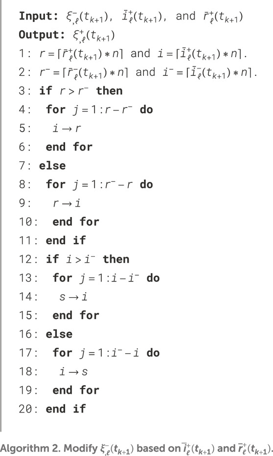
Algorithm 2. Modify ${\xi }_{,\ell }^{-}(t_{k+1})$ based on ${\bar{i}}_{\ell }^{+}(t_{k+1})$ and ${\bar{r}}_{\ell }^{+}(t_{k+1})$.

Let the result of ${\xi }_{,\ell }^{-}(t_{k+1})$ after correction using Algorithm 2 be denoted as ${\xi }_{,\ell }^{+}(t_{k+1})$.

The result of a single step in the System (Equation 2) has significant randomness. Here, we introduce a new parameter: the window length $L$, and assimilate the states $x^{+}(t_k)$ every $L$ steps.

The entire process of our algorithm is presented in Algorithm 3.

Algorithm 3

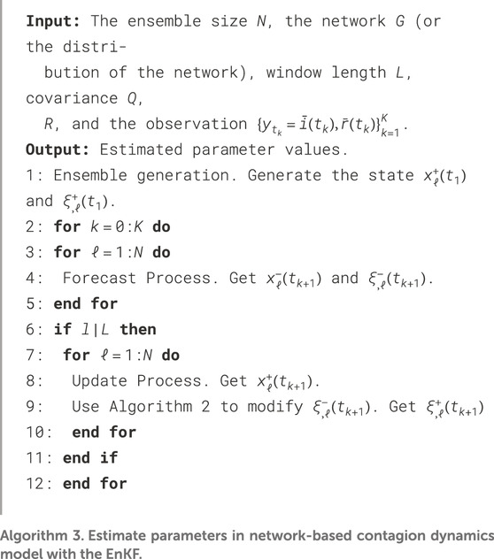
Algorithm 3. Estimate parameters in network-based contagion dynamics model with the EnKF.

3.2.5.5 Estimated result

We use the average of the states of the ensemble members as the estimation result of the algorithm: $i_{\mathit{est}}(t_k)=\frac{1}{N}{\displaystyle {\sum }_{\ell \in \{N\}}}\hspace{0.17em}{\bar{i}}_{\ell }^{+}(t_k)$ and $r_{\mathit{est}}(t_k)=\frac{1}{N}{\displaystyle {\sum }_{\ell \in \{N\}}}\hspace{0.17em}{\bar{r}}_{\ell }^{+}(t_k)$; in scenarios 1 and 3, ${\beta }_{\mathit{est}}(t_k)=\frac{1}{N}{\displaystyle {\sum }_{\ell \in \{N\}}}\hspace{0.17em}{g}^{-1}({\theta }_{1,\ell }^{+}(t_k))$ and ${\gamma }_{\mathit{est}}(t_k)=\frac{1}{N}{\displaystyle \sum _{\ell \in \{N\}}}{g}^{-1}({\theta }_{2,\ell }^{+}(t_k))$, and in Scenario 2, ${\beta }_{\mathit{est}}^{\prime }(t_k)=\frac{1}{N}{\displaystyle {\sum }_{\ell \in \{N\}}}\hspace{0.17em}{g}^{-1}({\theta }_{1,\ell }^{+}(t_k))$ and ${\gamma }_{\mathit{est}}^{\prime }(t_k)=\frac{1}{N}{\displaystyle {\sum }_{\ell \in \{N\}}}\hspace{0.17em}{g}^{-1}({\theta }_{2,\ell }^{+}(t_k))$.

4 Numerical simulation

4.1 Experiment setting

The proposed algorithm has been implemented using the Python programming language with the NDLib library for simulating the toy model. We conducted experiments on a machine equipped with an Intel(R) Core(TM) i7-10750H CPU running at 2.60 GHz, 32.0 GB of RAM, and a 1 TB SSD.

4.2 Experiment dataset

In scenarios 1 and 2, we use real network data to validate our algorithm. Specifically, we utilize the Internet Gnutella05 peer-to-peer network dataset, which contains 8,846 nodes and 31,839 arcs. The average node in- and out-degree is 3.5993, with a maximal node in-degree of 79 and a maximal node out-degree of 65. This dataset can be accessed from the following link: https://snap.stanford.edu/data/p2p-Gnutella05.html.

In Scenario 3, network $G$ is sampled from the following three types of synthetic networks:

• Erdős–Rényi random graph (ER): The graph $G(n,p_e)$ chooses each of the possible edges with probability $p_e$ among $n$ nodes.

• Watts–Strogatz small-world random graph (WS): The graph $G(n,d,p_w)$ is a small-world graph with $n$ nodes, where each node has $d$ adjacent neighbors. Then, edges are rewired with probability $p_w$.

• Barabási–Albert scale-free random graph (BA): The graph $G(n,m)$ is a scale-free graph with $n$ nodes, starting from an initial set of $m_0$ nodes. For each new node added, there are $m$ edges connecting it to existing nodes.

In Scenario 2, where each node has different parameters, we use the exponential distribution to sample ${\beta }_v$ and ${\gamma }_v$. This approach is similar to that described in [24]. In particular, the cumulative distribution functions (CDFs) of $D_1({\beta }^{\prime })$ and $D_2({\gamma }^{\prime })$ are given by ${\mathcal{F}}_{{\beta }^{\prime }}(x)=1-e^{-x/{\beta }^{\prime }}$ and ${\mathcal{F}}_{{\gamma }^{\prime }}(x)=1-e^{-x/{\gamma }^{\prime }}$, respectively. Here, ${\beta }_v$ and ${\gamma }_v$ are sampled from these distributions with parameters ${\beta }^{\prime }$ and ${\gamma }^{\prime }$, respectively.

4.3 Evaluation metrics

We define ${\{\bar{i}(t_k)\}}_{k=1}^K$ and ${\{\bar{r}(t_k)\}}_{k=1}^K$ as the observed average infection and recovery rates, respectively. The true parameter values are represented by ${\beta }_{\mathit{true}}$, ${\gamma }_{\mathit{true}}$, ${\beta }_{\mathit{true}}^{\prime }$ and ${\gamma }_{\mathit{true}}^{\prime }$. Meanwhile, the estimated values at time $t_k$ are denoted as $i_{\text{est}}(t_k)$, $r_{\text{est}}(t_k)$, ${\beta }_{\text{est}}(t_k)$, ${\gamma }_{\text{est}}(t_k)$, ${\beta }_{\text{est}}^{\prime }(t_k)$, and ${\gamma }_{\text{est}}^{\prime }(t_k)$. To verify the effectiveness of the algorithm, we assessed the assimilated data from two aspects:

(i) Measurement of the assimilation effect of observations:

$\begin{array}{cc}\hfill & \text{error}\left(obs\right)=\frac{1}{K}{\displaystyle \sum _{k=1}^K}\frac{{\left(i_{\mathit{est}}\left(t_k\right)-\bar{i}\left(t_k\right)\right)}^2}{\bar{i}{\left(t_k\right)}^2}+\frac{{\left(r_{\mathit{est}}\left(t_k\right)-\bar{r}\left(t_k\right)\right)}^2}{\bar{r}{\left(t_k\right)}^2}.\hfill \end{array}$

(ii) Measurement of the parameter estimation performance:

$\begin{array}{cc}\hfill & \text{error}\left(para\right)=\frac{1}{50}{\displaystyle \sum _{k=K-49}^K}\frac{{\left({\beta }_{\mathit{est}}\left(t_k\right)-{\beta }_{\mathit{true}}\right)}^2}{{\beta }_{\mathit{true}}^2}+\frac{{\left({\gamma }_{\mathit{est}}\left(t_k\right)-{\gamma }_{\mathit{true}}\right)}^2}{{\gamma }_{\mathit{true}}^2},\hfill \end{array}$

or in Scenario 2,

$\begin{array}{cc}\hfill & \text{error}\left(para\right)=\frac{1}{50}{\displaystyle \sum _{k=K-49}^K}\frac{{\left({\beta }_{\mathit{est}}^{\prime }\left(t_k\right)-{\beta }_{\mathit{true}}^{\prime }\right)}^2}{{{\beta }_{\mathit{true}}^{\prime }}^2}+\frac{{\left({\gamma }_{\mathit{est}}^{\prime }\left(t_k\right)-{\gamma }_{\mathit{true}}^{\prime }\right)}^2}{{{\gamma }_{\mathit{true}}^{\prime }}^2}.\hfill \end{array}$

4.4 Homogeneous model and known network

In this subsection, the network topology is explicitly known, and the model parameters are homogeneous across nodes, i.e., ${\beta }_v=\beta$ and ${\gamma }_v=\gamma$. This constitutes the simplest scenario, under which we consider four questions: (1) the performance of the algorithm in continuous-time dynamics; (2) the necessity of introducing network topology into the model; (3) the comparison between the ensemble Kalman filter and the particle filter algorithms; and (4) the optimal parameters for our algorithm. In this subsection, we use the Gnutella05 Internet peer-to-peer network as our network topology.

4.4.1 Performance of the algorithm in continuous-time dynamics

As shown in Section 3.2.3, the algorithm can be applied on the two continuous-time evolution simulation methods. We take $G$ as the Gnutella05 network, with $\beta =0.03$ and $\gamma =0.05$. We used both the simulation method based on the Gillespie algorithm and the random sampling-based simulation to generate observations and assimilate data. Since we cannot control the time intervals at which events are generated in the Gillespie-based simulation, we can only set a maximum simulation time. We set the maximum running time to 100. We conducted a total of 10 experiments, with an average of 1,984 time points generated in each experiment. For each experiment, we selected one time point for every 19 time points as an observation, resulting in a total of 101 selected nodes. For the random sampling-based simulation, we set the time interval to 1, i.e., $t_k=k$ and $K=100$.

Figures 1, 2, respectively, demonstrate the effectiveness of our algorithm based on the two continuous-time simulation methods mentioned above (Gillespie-based and random-sampling-based). For the Gillespie-based simulation in Figure $1,\text{error}(obs)=8.8034e-2$ and $\text{error}(para)=4.4327e-3$; for the random-sampling-based simulation in Figure 2, $\text{error}(obs)=6.1656e-2$ and $\text{error}(para)=4.3138e-3$.

Figure 1

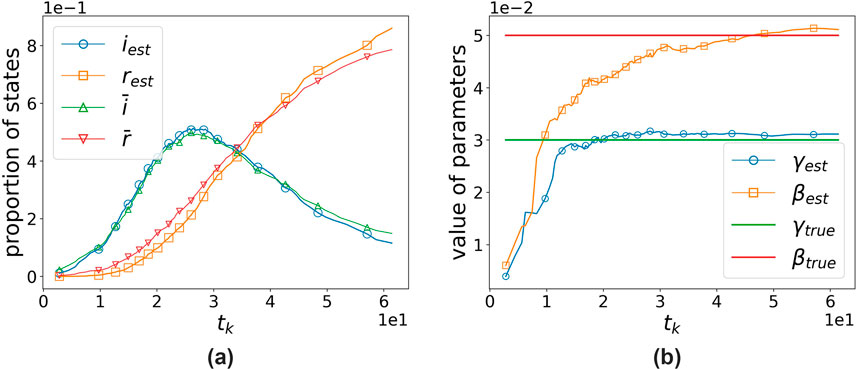
Figure 1. Performance of the algorithm when using the Gillespie-based simulation method. $\bar{i}$ and $\bar{r}$ are the observations, while ${\beta }_{\mathit{true}}$ and ${\gamma }_{\mathit{true}}$ are the true parameter values. $\text{error}(obs)=8.8034e-2$, and $\text{error}(para)=4.4327e-3$. (a) States’ proportion vs. time. (b) Parameters’ value vs. time.

Figure 2

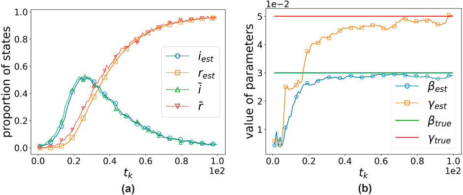
Figure 2. Performance of the algorithm when using the random-sampling-based simulation method. $\bar{i}$ and $\bar{r}$ are the observations, while ${\beta }_{\mathit{true}}$ and ${\gamma }_{\mathit{true}}$ are the true parameter values. $\text{error}(obs)=6.1656e-2$ and $\text{error}(para)=4.3138e-3$. (a) States’ proportion vs. time. (b) Parameters’ value vs. time.

It can be observed that our algorithm’s estimates are close to the true values using both simulation methods. The assimilation effect using the Gillespie-based simulation method is slightly worse, which may be because the time intervals generated using the Gillespie-based method are not uniform, and thus, the magnitude of each correction cannot be controlled. The average of the results from 10 experiments shows that, for the Gillespie-based simulation, $\text{error}(obs)=9.4176e-2$ and $\text{error}(para)=4.2962e-3$; for the random-sampling-based simulation, $\text{error}(obs)=3.6788e-2$ and $\text{error}(para)=4.3795e-3$. This demonstrates that our algorithm is also effective when applied to continuous-time simulation methods.

We compare the differences among the three simulation methods in the following paragraph. Figure 3 illustrates the performance of the three different simulation methods described in Section 3.2.3 when $\beta =0.03$, $\gamma =0.05$, and the evolution time is 100. The simulation results of these three methods are quite close.

Figure 3

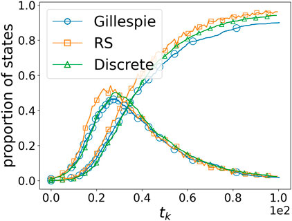
Figure 3. Comparison of the three simulation methods. “Gillespie,” “RS,” and “Discrete” refer to the Gillespie-based simulation, random-sampling-based simulation, and discrete simulation, respectively.

However, there is a significant difference in the running time. The Gillespie-based simulation method generates nearly 2,000 time points each time, with an average running time of 675.2 s for the entire simulation process; the random-sampling-based simulation method, when the number of nodes is very large, consumes a considerable amount of time on each sampling, with an average running time of 136.7 s; the discrete simulation method is the fastest, with an average running time of 10.3 s.

Given that the simulation results are quite similar and that continuous-time dynamics can also be simulated using the discrete simulation method by adjusting the time intervals during discretization (since computations are always discrete in practice), for the sake of efficiency, the discrete simulation method is consistently used in the subsequent experiments.

4.4.2 Necessity of incorporating network topology

When network topology is incorporated, the model’s complexity increases compared to the baseline. Nevertheless, if the standard SIR model remains capable of producing accurate parameter estimates even when observational dynamics encompass network effects, the enhanced model would prove redundant and entail unnecessary computational overhead.

In this subsection, we generate observational data using the dynamics (Equation 2) that incorporate network effects and then estimate parameters through the standard SIR model coupled with the EnKF, replicating the methodology in [9]. With $\gamma$ fixed at 0.002 and$\beta$ varying from 0.005 to 0.01 in 0.001 increments, we set the initial infection rate to 0.002 and perform 3,000 iterations. Figure 4 displays single-experiment results for $\beta =0.006$, where $i_{\mathit{ori}}$ and $r_{\mathit{ori}}$ denote estimated average infection/recovery rates, ${\beta }_{\mathit{ori}}$ and ${\gamma }_{\mathit{ori}}$ represent parameter estimates, $\bar{i}$ and $\bar{r}$ are observed values, while ${\beta }_{\mathit{true}}$ and ${\gamma }_{\mathit{true}}$ indicate true parameter values.

Figure 4

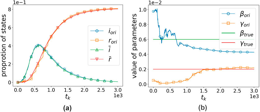
Figure 4. Original SIR model’s performance when $\gamma =0.002$ and $\beta =0.006$. $\bar{i}$ and $\bar{r}$ are the observations; ${\beta }_{\mathit{true}}$ and ${\gamma }_{\mathit{true}}$ are the true parameter values, and $i_{\mathit{ori}}$, $r_{\mathit{ori}}$, ${\beta }_{\mathit{ori}}$, and ${\gamma }_{\mathit{ori}}$ are the estimations with the original SIR model. (a) States’ proportion vs. time. (b) Parameters’ value vs. time.

The algorithm exhibits clear convergence. For each parameter set, we conducted 10 independent trials, with the final 50 time-step averages serving as steady-state estimates. Figure 5 displays the experimental outcomes, where the x-axis denotes the six $\beta$ values (0.005–0.01 in 0.001 increments) and error bars show the range (minimum to maximum) with mean values across trials.

Figure 5

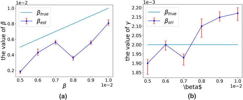
Figure 5. Comparison of true parameters and estimated parameters under the original SIR model. (a) True $\beta$ vs. estimated $\beta$. (b) True $\gamma$ vs. estimated $\gamma$.

It can be clearly observed that the original SIR model systematically underestimates the transmission rate $\beta$. This is because, when considering the network topology, each node can only interact with its adjacent nodes. In contrast, the original SIR model assumes that each node can interact with any other node. This assumption corresponds to a complete graph in terms of network topology, which amplifies the virus’s transmission capability and leads to an underestimation of the virus’s infection capability. Therefore, it is methodologically imperative to use a model based on network topology.

4.4.3 Comparison with algorithms based on particle filter

Our algorithm can also be deployed on particle filtering. We compared the performance between the EnKF- and the PF-based algorithms, with the same number of particles, for ensemble sizes of 50 and 100. The observational data are derived from the following parameters: $\beta =0.005$, $\gamma =0.002$, the initial infection rate is 0.002, and iteration count $K=\mathrm{3,000}$.

Table 3 shows the performance of the two algorithms. Figures 6, 7 visualize the assimilation effects of the two algorithms when the ensemble sizes are 50 and 100, respectively. $i_{\mathit{EnKF}}$, $r_{\mathit{EnKF}}$, ${\beta }_{\mathit{EnKF}}$, and ${\gamma }_{\mathit{EnKF}}$ are the estimates of the average infection rate, average recovery rate, $\beta$, and $\gamma$, respectively, obtained using the EnKF-based algorithm. Similarly, $i_{PF}$, $r_{PF}$, ${\beta }_{PF}$, and ${\gamma }_{PF}$ are the estimates obtained using the PF-based algorithm. $\bar{i}$ and $\bar{r}$ are the observed values, while ${\beta }_t$ and ${\gamma }_t$ are the true values of the parameters $\beta$ and $\gamma$, respectively.

Table 3

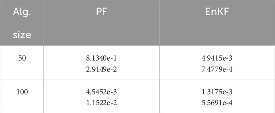
Table 3. Algorithm performance under different filters with sizes of 50 and 100. In each cell, the upper part shows $\text{error}(obs)$, and the lower part shows $\text{error}(para)$.

Figure 6

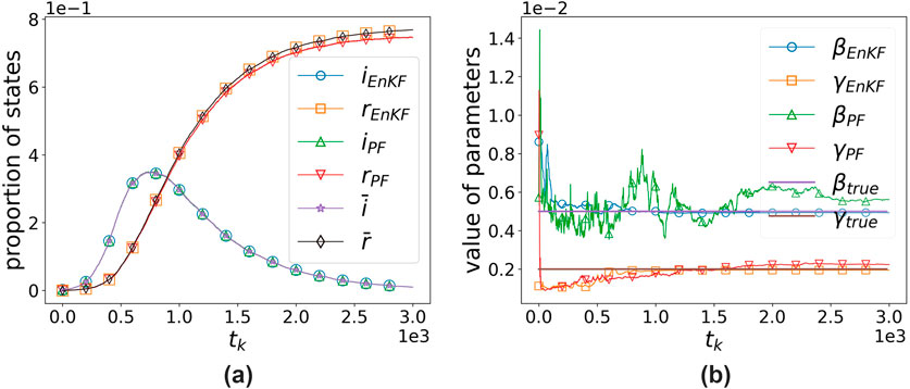
Figure 6. Comparison of algorithms based on the EnKF and PF with size 50. (a) States’ proportion vs. time. (b) Parameters’ value vs. time.

Figure 7

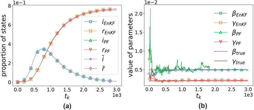
Figure 7. Comparison of algorithms based on the EnKF and PF with size 100. (a) States’ proportion vs. time. (b) Parameters’ value vs. time.

It can be observed that both algorithms perform well in assimilating observational data, with the EnKF-based algorithm showing a slight advantage. However, in terms of parameter estimation, EnKF significantly outperforms PF, with results differing by two orders of magnitude. The EnKF also converges faster and exhibits greater stability, yielding satisfactory results even with an ensemble size of 50. In contrast, PF only shows slightly better performance when the number of particles reaches 100, and its efficiency is far lower than that of the EnKF.

4.4.4 Optimal parameters for this algorithm

We then explore the impact of different hyperparameters: the number of ensemble members $N$, the covariance of the system noises $Q_{\mathrm{3,3}}$, the covariance of the observation noise $R_{\mathrm{1,1}}$, and the window length $L$ on the estimation effect.

We set the observation’s parameters as ${\beta }_t=0.005$, ${\gamma }_t=0.002$, the initial infection rate $i_0=0.002$, and the number of iterations $K=\mathrm{3,000}$. We seek the optimal parameters through empirical trials and determine the best values to be $Q=1e-4$, $R=5e-4$, $N=50$, and $L=10$. Table 4 lists the performance under different parameter settings. In Table 4, each cell indicates the value of the changed parameter and its performance, with all other parameters remaining the same as the best parameter setting. The results are obtained by taking the average of 10 independent experiments.

Table 4

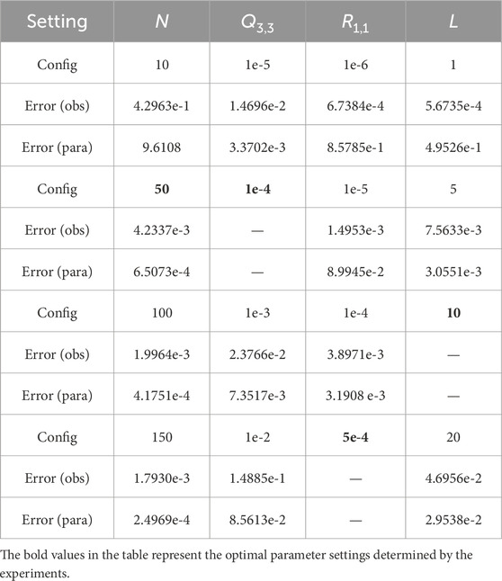
Table 4. Algorithm performance under different parameter settings. Each cell has only one value that differs from the optimal parameters.

Figure 8 illustrates the algorithm’s fitting of observations and estimation of parameters under the optimal parameters. It can be observed that the algorithm exhibits excellent fitting performance for the observations, and the estimated parameters converge to the actual values, which validates our algorithm. For easy comparison, in the example shown in the figure, $\text{error}(obs)=4.5731e-3$ and $\text{error}(para)=6.3527e-4$. The optimal parameters were used in the following scenarios.

Figure 8

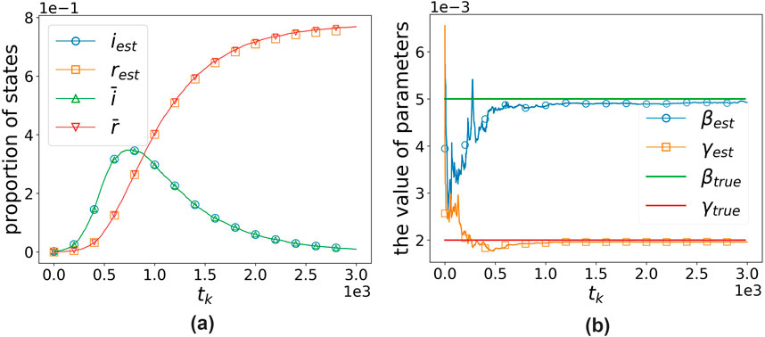
Figure 8. Algorithm’s fitting effect and the estimation effect on parameters under the optimal parameters when $\beta =0.005$ and $\gamma =0.002$, where $\text{error}(obs)=4.5731e-3$ and $\text{error}(para)=6.3527e-4$. (a) States’ proportion vs. time. (b) Parameters’ value vs. time.

As shown in Table 4, the larger the ensemble size $N$, the better the performance of the algorithm. However, since the algorithm is serial, doubling the ensemble size will double the computation time.

Therefore, we set the ensemble size to 50 as its performance is not significantly different from that of ensemble sizes of 100 or 150. When the observational covariance $R_{\mathrm{1,1}}$ is smaller or the window length $L$ is shorter, the algorithm’s assimilation of observational data is better. However, this leads to worse parameter estimation. Thus, intermediate values of $R_{\mathrm{1,1}}=5e-4$ and $L=10$ are chosen. Additionally, when the window length is too long, both the assimilation and observation effects of the algorithm deteriorate significantly. With these parameter settings, our algorithm can complete the optimization process of 3,000 time steps within 40 min.

4.5 Heterogeneous model and known network

We assume that the node parameters are different but sampled from the same exponential distribution: the cumulative distribution functions of $D_1({\beta }^{\prime })$ and $D_2({\gamma }^{\prime })$ are ${\mathcal{F}}_{{\beta }^{\prime }}(x)=1-e^{-x/{\beta }^{\prime }}$ and ${\mathcal{F}}_{{\gamma }^{\prime }}(x)=1-e^{-x/{\gamma }^{\prime }}$, respectively. We still used the Internet Gnutella05 peer-to-peer network and set $Q_{\mathrm{3,3}}=1e-4$, $R_{\mathrm{1,1}}=5e-4$, $N=50$, and $L=10$. First, we set ${\beta }^{\prime }=0.006$ and ${\gamma }^{\prime }=0.003$, and the results are shown in Figure 9. In the experiment shown in Figure 9, $\text{error}(obs)=5.7584e-2$ and $\text{error}(para)=2.4573e-2$. It indicates that our algorithm converges to the true values and can estimate the states well; however, the estimations for the parameters are not as accurate as those of the homogeneous model. The accuracies of the experiments in Figure 9 are $\text{error}(para)=0.27567$ and $\text{error}(obs)=0.02743$.

Figure 9

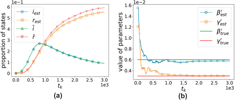
Figure 9. Algorithm’s fitting effect and the estimation effect on hyperparameters. ${\beta }_{\mathit{true}}^{\prime }=0.006$, ${\gamma }_{\mathit{true}}^{\prime }=0.003$, $\bar{i}$, and $\bar{r}$ are the true values, while ${\beta }_{\mathit{est}}^{\prime }$, ${\gamma }_{\mathit{est}}^{\prime }$, $i_{\mathit{est}}$, and $r_{\mathit{est}}$ are our estimations. In the experiment, $\text{error}(obs)=5.7584e-2$ and $\text{error}(para)=2.4573e-2$. (a) States’ proportion vs. time. (b) Parameters’ value vs. time.

We then investigated the impact of different parameters on the accuracy. Table 5 lists the accuracy of the algorithm when ${\beta }^{\prime }=0.005,0.01,0.015,0.02,0.1$ and ${\gamma }^{\prime }=0.003,0.006,0.009,0.012,0.2$. We can observe that when the parameter is small, the algorithm performs well (not inferior to Figure 9); however, when the parameter is large, the algorithm performs poorly. We believe that this may be due to the rapid convergence rate of the SIR model caused by the large parameter values, which does not allow the algorithm sufficient time to update the information.

Table 5

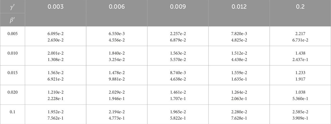
Table 5. Algorithm’s performance under different ${\beta }^{\prime }$ and ${\gamma }^{\prime }$. In each cell, the top value is $\text{error}(obs)$, and the bottom value is $\text{error}(para)$. Each value is obtained by taking the average of 10 independent repeated experiments.

Moreover, the success of our algorithm suggests that when there are sufficient nodes in the network, the infection situation of computer viruses may not be related to the specific defense capabilities of the nodes or the infection capabilities of the viruses but rather to the probability distribution of defense and infection capabilities. This is consistent with the ideas of some studies that used statistical physics to study contagion dynamics [11].

4.6 Different networks

In this subsection, we assume that the model is homogeneous and that the network is unknown, but we know that it has a specific structure, and the structural parameters are known. We used this hyperparameter to generate new random graphs for each ensemble member to estimate the model.

We consider three types of synthetic random networks: Erdős–Rényi graph $G(n,p_e)$, Watts–Strogatz graph $G(n,d,p_w)$, and Barabási–Albert scale-free graph $G(n,m)$. To make a horizontal comparison among different types of networks, we considered the variation in the average degree of the networks. We generate networks with 5,000 nodes and average degrees of 10, 100, 200, and 300, then form observational data with $\beta =0.002$ and $\gamma =0.001$, and set the parameters $Q_{\mathrm{3,3}}=1\times 10^{-4}$, $R_{\mathrm{1,1}}=5\times 10^{-4}$, $N=50$, and $L=10$.

Figure 10 illustrates the algorithm’s performance in separate experiments conducted on three distinct networks with 5,000 nodes, an average degree of 10, and parameters $\beta =0.002$ and $\gamma =0.001$. The experimental results are as follows: on the Erdős–Rényi graph, $\text{error}(obs)=2.1672e-3$ and $\text{error}(para)=4.2538e-2$; on the Watts–Strogatz graph, $\text{error}(obs)=3.7961e-3$ and $\text{error}(para)=6.6674e-2$; and on the Barabási–Albert graph, $\text{error}(obs)=1.0513e-3$ and $\text{error}(para)=5.7914e-3$. Table 6 lists all the accuracy metrics: $\text{error}(obs)$ and $\text{error}(para)$ for reference, where each value was obtained by averaging over 10 repeated independent experiments.

Figure 10

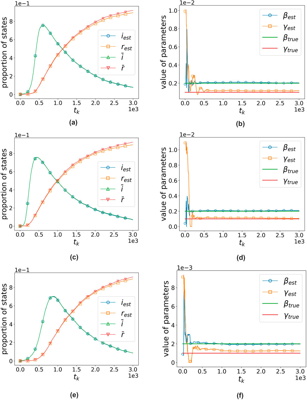
Figure 10. Algorithm’s performance on three random graphs with 5,000 nodes and an average degree of 10 when $\beta =0.002$ and $\gamma =0.001$. (a) States’ proportion vs. time. (b) Parameters’ value vs. time. Performance on the Erdős–Rényi random graph, with $\text{error}(obs)=2.1672e-3$ and $\text{error}(para)=4.2538e-2$. (c) States’ proportion vs. time. (d) Parameters’ value vs. time. Performance on the Watts–Strogatz random graph, with $\text{error}(obs)=3.7961e-3$ and $\text{error}(para)=6.6674e-2$. (e) States’ proportion vs. time. (f) Parameters’ value vs. time. Performance on the Barabási–Albert random graph, with $\text{error}(obs)=1.0513e-3$ and $\text{error}(para)=5.7914e-3$.

Table 6

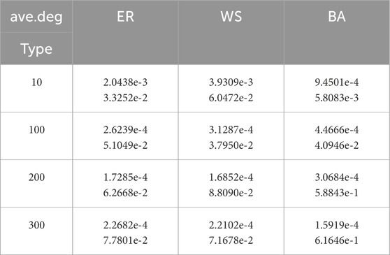
Table 6. Performance of the algorithm when $\beta =0.002$ and $\gamma =0.001$. In each cell, the top value is $\text{error}(obs)$, and the bottom value is $\text{error}(para)$.

It can be observed that even without knowing the specific network structure, our algorithm performs well across all three types of networks, demonstrating its robustness. Meanwhile, as shown in the table, when the average degree increases (e.g., to 200 and 300), the performance of our algorithm in estimating parameters on BA networks decreases significantly. We speculate that this is because BA networks are heterogeneous, with highly uneven degree distributions and a significant number of nodes with very high degrees. These high-degree nodes have a substantial impact on the spread of the virus. As the average degree increases, the heterogeneity of the network also increases, rendering the method of averaging less suitable for estimating network parameters. This, in turn, leads to a decrease in the performance of our algorithm.

4.7 SIS model

In the previous section, we focused on the SIR model; however, it should be noted that our algorithm is not only applicable to the SIR model but can also be used for other classic epidemic models. In this subsection, we use our algorithm to estimate a network-based SIS model [19]. We assume that any node $v$ in the network $G$ can only be in one of the following two states at the same time: 0 (susceptible state) or 1 (infective state), and the evolution of the probabilities of node states obeys the following dynamical system: for node $v\in V$,

$\begin{array}{cc}\hfill \frac{d{s}_v\left(t\right)}{dt}& =-\left(1-\prod _{u\in V,u\ne v}\left(1-{\beta }_u{a}_{u,v}{i}_v\left(t\right)\right)\right)s_v\left(t\right)+{\lambda }_v{i}_v\left(t\right)\hfill \\ \hfill \frac{d{i}_v\left(t\right)}{dt}& =\left(1-\prod _{u\in V,u\ne v}\left(1-{\beta }_u{a}_{u,v}{i}_v\left(t\right)\right)\right)s_v\left(t\right)-{\lambda }_v{i}_v\left(t\right)\hfill \end{array}$

where ${\beta }_v$ and ${\lambda }_v$ for $v\in V$ are the infection rate and recovery rate for node $v$, respectively. Using a method similar to that in Section 3.2, we can estimate this dynamical model using the EnKF.

In the estimation experiment, we used a 5,000-node ER network, with an average degree of 10. The average infection rate $\bar{i}(t_k)$, the number of new infections at each time step $\mathrm{\Delta }i(t_k)$, the infection rate $\beta$, and the recovery rate $\lambda$ were used as the states. We set $\beta =0.002$ and $\lambda =0.001$, and the iteration time $K=\mathrm{3,000}$ to generate the observations. In the estimation process, we set $Q_{\mathrm{3,3}}=1e-4$, $R_{\mathrm{1,1}}=5e-4$, $N=50$, and $L=10$. As mentioned previously, the algorithm updates the true input of the dynamics $\xi (t_k)$ based on the average infection rate $\bar{i}(t_k)$ for every $L$ time steps.

The two subfigures in Figure 11, respectively, show the algorithm’s data assimilation of observational states and its parameter estimation effectiveness. ${\beta }_{\mathit{true}}$ and ${\lambda }_{\mathit{true}}$ are the true parameter values; $\bar{i}$ and $\mathrm{\Delta }i$ are the observations; $i_{\mathit{est}}$, $\mathrm{\Delta }{i}_{\mathit{est}}$, ${\beta }_{\mathit{est}}$, and ${\gamma }_{\mathit{est}}$ are the estimated values. In subfigure (a), due to the large magnitude difference between $\mathrm{\Delta }i$ and $\bar{i}$, the y-axis for $\bar{i}$ is placed on the right side of subfigure (a), while the y-axis for $\mathrm{\Delta }i$ is placed on the left. It can be observed that our algorithm also performs well on the network-based SIS model.

Figure 11

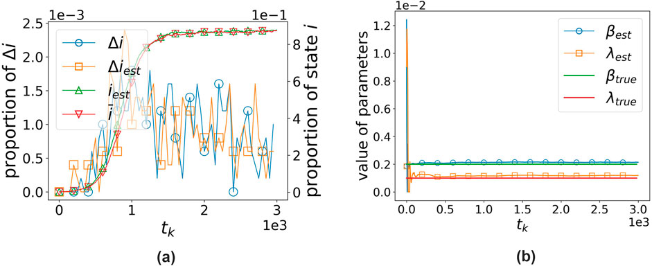
Figure 11. Algorithm performance on the network-based SIS model. (a) States’ proportion vs. time. (b) Parameters’ value vs. time.

5 Conclusion and discussion

This study proposes a data assimilation algorithm to estimate network-based contagion dynamical models, including the states, parameters, and hyperparameters. We validate the performance of the algorithm in three scenarios, demonstrating its powerful capabilities and suggesting that when the network size is sufficiently large, the dynamical behavior may be independent of the specific network and parameters, instead depending on their distributions.

Although our algorithm performed well in experiments, it still has obvious limitations when applied in practice.

(1) Due to the lack of relevant real-world data, we cannot validate the effectiveness of our algorithm on public datasets as other algorithm papers do. Experiments can only be conducted using synthetic data, suggesting that we are not certain about how our algorithm will perform in practical applications.

(2) The method of data assimilation is highly dependent on the choice of the model. For existing data, we must precisely know the underlying model to make accurate predictions and estimates. However, due to the lack of real-world data, we are unable to determine how the algorithm performs on real data. The algorithm also requires information about the specific network structure. In the three scenarios, we know either the exact network structure or that the network structure comes from a specific distribution, which is relatively difficult in reality.

(3) When the underlying dynamics converge too rapidly, our algorithm does not have sufficient time to update the states and acquire information, thus resulting in mediocre performance. We need to understand at what convergence rate of the dynamics our algorithm can ensure accuracy.

(4) There is a lack of theoretical guarantees regarding the reliability of the algorithm and the choice of hyperparameters, and there is also a general lack of publicly available and reliable network-topology-based time series datasets in the field of contagion dynamics. This makes it difficult to validate our algorithm, along with other theoretical results, on public datasets. Ensuring the theoretical reliability of our algorithm and developing methods for collecting data to construct useful datasets will both be important directions for our future research.

Data availability statement

The original contributions presented in the study are included in the article/supplementary material; further inquiries can be directed to the corresponding author.

Author contributions

YW: Data curation, Formal Analysis, Investigation, Software, Validation, Visualization, Writing – original draft, and Writing – review and editing. WL: Conceptualization, Formal Analysis, Funding acquisition, Investigation, Methodology, Resources, Supervision, and Writing – original draft.

Funding

The author(s) declare that financial support was received for the research and/or publication of this article. This work is supported by the Science and Technology Commission of Shanghai Municipality (No. 23JC1400800).

Conflict of interest

The authors declare that the research was conducted in the absence of any commercial or financial relationships that could be construed as a potential conflict of interest.

Generative AI statement

The author(s) declare that Generative AI was used in the creation of this manuscript. The author(s) verify and take full responsibility for the use of generative AI in the preparation of this manuscript. Generative AI was used Kimi.

Publisher’s note

All claims expressed in this article are solely those of the authors and do not necessarily represent those of their affiliated organizations, or those of the publisher, the editors and the reviewers. Any product that may be evaluated in this article, or claim that may be made by its manufacturer, is not guaranteed or endorsed by the publisher.

References

1. Chakrabarti D, Wang Y, Wang C, Leskovec J, Faloutsos C. Epidemic thresholds in real networks. ACM Trans Inf Syst Security (Tissec) (2008) 10(4):1–26. doi:10.1145/1284680.1284681

CrossRef Full Text | Google Scholar

2. Javier Cocucci T, Pulido M, Aparicio JP, Ruíz J, Simoy MI, Rosa S. Inference in epidemiological agent-based models using ensemble-based data assimilation. PloS one (2022) 17(3):e0264892. doi:10.1371/journal.pone.0264892

PubMed Abstract | CrossRef Full Text | Google Scholar

3. Cohen JE. Infectious diseases of humans: dynamics and control. JAMA The J Am Med Assoc (1992) 268(23):3381. doi:10.1001/jama.1992.03490230111047

CrossRef Full Text | Google Scholar

4. Epstein JM, Parker J, Cummings D, Hammond RA. Coupled contagion dynamics of fear and disease: mathematical and computational explorations. PloS one (2008) 3(12):e3955. doi:10.1371/journal.pone.0003955

PubMed Abstract | CrossRef Full Text | Google Scholar

5. Ghostine R, Gharamti M, Hassrouny S, Hoteit I. An extended seir model with vaccination for forecasting the covid-19 pandemic in Saudi Arabia using an ensemble kalman filter. Mathematics (2021) 9(6):636. doi:10.3390/math9060636

CrossRef Full Text | Google Scholar

6. Daniel TG. A general method for numerically simulating the stochastic time evolution of coupled chemical reactions. J Comput Phys (1976) 22(4):403–34. doi:10.1016/0021-9991(76)90041-3

CrossRef Full Text | Google Scholar

7. Herbert W. The mathematics of infectious diseases. SIAM Rev (2000) 42:599–653. doi:10.1137/s0036144500371907

CrossRef Full Text | Google Scholar

8. Hoteit I, Pham D-T, Triantafyllou G, Korres G. A new approximate solution of the optimal nonlinear filter for data assimilation in meteorology and oceanography. Monthly Weather Rev (2008) 136(1):317–34. doi:10.1175/2007mwr1927.1

CrossRef Full Text | Google Scholar

9. Huáng W, Provan GM. An improved state filter algorithm for sir epidemic forecasting. In: European conference on artificial intelligence (2016). doi:10.3233/978-1-61499-672-9-524

CrossRef Full Text | Google Scholar

10. Matt J, Eames KT. Networks and epidemic models. J R Soc Interf (2005) 2(4):295–307. doi:10.1098/rsif.2005.0051

CrossRef Full Text | Google Scholar

11. Newman MEJ, Newman MEJ. Spread of epidemic disease on networks. Phys Rev E, Stat nonlinear, soft matter Phys (2002) 66(1 Pt 2):016128. doi:10.1103/PhysRevE.66.016128

CrossRef Full Text | Google Scholar

12. Mark EJN. Estimating network structure from unreliable measurements. Phys Rev E (2018) 98(6):062321. doi:10.1103/physreve.98.062321

CrossRef Full Text | Google Scholar

13. Newman MEJ. Network structure from rich but noisy data. Nat Phys (2018) 14(6):542–5. doi:10.1038/s41567-018-0076-1

CrossRef Full Text | Google Scholar

14. Nowzari C, Preciado VM, Pappas GJ. Analysis and control of epidemics: a survey of spreading processes on complex networks. IEEE Control Syst Mag (2016) 36(1):26–46. doi:10.1109/MCS.2015.2495000

CrossRef Full Text | Google Scholar

15. Paré PE, Vrabac D, Sandberg H, Johansson KH. Analysis, online estimation, and validation of a competing virus model. In: 2020 American control conference (ACC) (2020). p. 2556–61. doi:10.23919/ACC45564.2020.9147568

CrossRef Full Text | Google Scholar

16. Ran Y, Deng X, Wang X, Jia T. A generalized linear threshold model for an improved description of the spreading dynamics. Chaos: An Interdiscip J Nonlinear Sci (2020) 30(8):083127. doi:10.1063/5.0011658

PubMed Abstract | CrossRef Full Text | Google Scholar

17. Shaman J, Karspeck A. Forecasting seasonal outbreaks of influenza. Proc Natl Acad Sci (2012) 109(50):20425–30. doi:10.1073/pnas.1208772109

PubMed Abstract | CrossRef Full Text | Google Scholar

18. Travieso G, Costa Lda F. Spread of opinions and proportional voting. Phys Rev E—Statistical, Nonlinear, Soft Matter Phys (2006) 74(3):036112. doi:10.1103/PhysRevE.74.036112

CrossRef Full Text | Google Scholar

19. Xu M, Da G, Xu S. Cyber epidemic models with dependences. Internet Mathematics (2015) 11(1):62–92. doi:10.1080/15427951.2014.902407

CrossRef Full Text | Google Scholar

20. Xu S. Cybersecurity dynamics. In: Proceedings of the 2014 symposium and bootcamp on the science of security, HotSoS ’14. New York, NY, USA: Association for Computing Machinery (2014). doi:10.1145/2600176.2600190

CrossRef Full Text | Google Scholar

21. Xu S. Cybersecurity dynamics: a foundation for the science of cybersecurity. Proactive dynamic Netw defense (2019) 1–31. doi:10.1007/978-3-030-10597-6_1

CrossRef Full Text | Google Scholar

22. Xu S, Lu W, Xu L. Push-and pull-based epidemic spreading in networks: thresholds and deeper insights. ACM Trans Autonomous Adaptive Syst (Taas) (2012) 7(3):1–26. doi:10.1145/2348832.2348835

CrossRef Full Text | Google Scholar

23. Yang W, Karspeck AR, Shaman JL. Comparison of filtering methods for the modeling and retrospective forecasting of influenza epidemics. PLoS Comput Biol (2014) 10:e1003583. doi:10.1371/journal.pcbi.1003583

PubMed Abstract | CrossRef Full Text | Google Scholar

24. Zhang W, Chen B, Feng J, Lu W. On a framework of data assimilation for hyperparameter estimation of spiking neuronal networks. Neural Networks (2024) 171:293–307. doi:10.1016/j.neunet.2023.11.016

PubMed Abstract | CrossRef Full Text | Google Scholar

25. Zheng R, Lu W, Xu S. Preventive and reactive cyber defense dynamics is globally stable. IEEE Trans Netw Sci Eng (2017) 5(2):156–70. doi:10.1109/tnse.2017.2734904

CrossRef Full Text | Google Scholar