A survey of GNSS receiver autonomous integrity monitoring: Research status and opportunities

Integrity monitoring is crucial in applications closely related to the safety of human life and property, such as aviation, maritime navigation, autonomous driving, and rail transportation. Receiver autonomous integrity monitoring (RAIM) has attracted significant attention due to its comprehensive monitoring coverage and fast alerting capability. The paper provides a comprehensive review of RAIM algorithms for global navigation satellite system (GNSS) positioning applications. The parameters related to integrity assessment and typical fault detection and exclusion methods are reviewed, and RAIM is categorized into three types of methods: error probability distribution model-based, set representation-based, and machine learning-based. The latest state-of-the-art research, along with the strengths and shortcomings of each type of method, is presented for each type. The opportunities for the future development of RAIM are analyzed in the light of current challenges and existing results, aiming to promote further research and provide effective assurance for GNSS integrity.

1 Introduction

The global navigation satellite system (GNSS) offers many advantages, such as all-weather, all-time, and global coverage, providing accurate and extensive positioning, navigation, and timing services for aviation [1], maritime navigation [2], railway transport [3], and autonomous driving [4]. Among these, integrity is one of the key criteria for evaluating GNSS performance. It is used to assess the trustworthiness of the navigation system, and its concept originally came from the field of aviation, aiming to provide highly reliable navigation and positioning information for civil aviation users. With the widespread application of GNSS in fields closely related to the safety of human lives and property, the concept of integrity has been expanded to other areas and has attracted much attention.

Integrity is defined as the ability to alert the user in a timely manner when the performance of the navigation information provided by GNSS fails to meet specified requirements [5, 6]. In January 2024, two ship groundings occurred in the Israeli ports of Haifa and Ashdod, as a result of excessive global positioning system (GPS) positioning deviation but the receivers did not warn the crews in time [7], which shows that safeguarding GNSS integrity is crucial for the safety of human lives and property. On the other hand, due to the vulnerability of the GNSS signals themselves, they are highly susceptible to jamming and spoofing. On 6 September 2024, OPSGROUP, an organization of aviation practitioners, compiled statistics on GPS spoofing in civil aviation, and the data showed that in the first three-quarters of 2024, an average of up to 1,500 flights were subjected to GPS spoofing every day [8]. The frequent occurrence of jamming and spoofing events will seriously weaken GNSS integrity, at the same time, ephemeris and clock failures, ionospheric and tropospheric fluctuations, and common multipath and non-line-of-sight (NLOS) signals in urban canyons may pose a threat to GNSS integrity, leading users to incorrectly believe and adopt navigation information with excessive errors, which can jeopardize the safety of human life and property. Therefore, providing accurate and reliable integrity services for GNSS users is an urgent issue, and integrity monitoring of GNSS is crucial and irreplaceable.

Depending on the stage of implementation of integrity monitoring, it can be divided into system-level and user-level methods. System-level methods rely on integrity information broadcast by satellite-based or ground-based monitoring stations. User-level methods, on the other hand, do not rely on external information or facilities, but only utilize their own redundant measurement information for integrity monitoring [9], and their main means of implementation is receiver autonomous integrity monitoring (RAIM). As shown in Figure 1, RAIM is theoretically able to monitor faults and abnormalities in the space segment, signal propagation segment, and user segment, with a comprehensive monitoring scope. Additionally, because RAIM is directly deployed at the user terminal, it can respond quickly to all kinds of faults and alert the user in time, and the response speed is usually much better than that of system-level integrity monitoring methods.

Figure 1

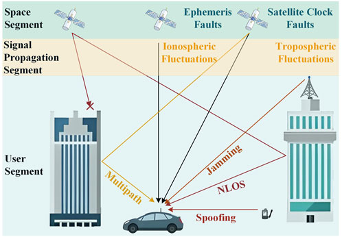
Figure 1. Faults or anomalies that may threaten integrity.

Several review works have summarized the research progress of RAIM. For instance [5], focuses on the advancements of RAIM in aviation [6], summarizes the integrity detection algorithms used in urban canyon environments [9], systematically reviews the integrity monitoring methods in GNSS and inertial navigation system (INS) integrated navigation for autonomous driving applications, and [10] highlights the progress in autonomous integrity monitoring within multi-source fusion navigation. However, these works do not provide a systematic overview of the more novel machine learning (ML)-based and set representation-based RAIM algorithms. Furthermore, many innovative developments in traditional RAIM have emerged, which are not covered in the existing reviews.

Therefore, this paper systematically describes the state-of-the-art RAIM algorithms for GNSS positioning applications. The remaining chapters are organized as follows: Section 2 reviews the parameters related to integrity assessment and typical fault detection and exclusion (FDE) methods. Section 3 introduces the state-of-the-art of three types of RAIMs: those based on the error probability distribution models, set representation, and ML, respectively, and analyzes the strengths and weaknesses of each. Section 4 examines the future development opportunities for RAIM by considering current challenges and existing research results. Finally, Section 5 provides conclusions and future outlooks.

2 Basic definition and theory

2.1 Integrity performance evaluation and related parameters

Four metrics—accuracy, integrity, continuity, and availability—are usually used to evaluate GNSS navigation performance, and the relationship between them can be represented by the navigation performance pyramid [6], as shown in Figure 2.

Figure 2

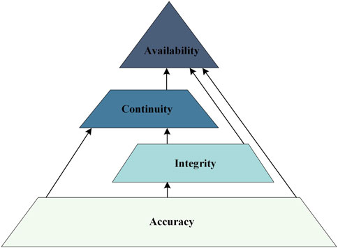
Figure 2. Navigation performance pyramid [6].

Among them, integrity is used to assess the trustworthiness of GNSS, which is measured by a series of parameters such as alert limit (AL), time to alert (TTA), integrity risk (IR), protection level (PL), etc. [6, 11], taking the positioning application as an example, these parameters are defined as follows:

AL: The maximum tolerable position error (PE), usually preset according to user requirements. Different requirements often exist in the horizontal and vertical directions, so it can be further divided into horizontal alert limit (HAL) and vertical alert limit (VAL).

TTA: The maximum tolerable time from when the PE exceeds the AL to when the user receives an alert.

IR: The maximum tolerable probability that the PE exceeds the AL but the user is not alerted within the TTA. This is usually given in terms of per hour or per mile [9]. Alternatively, IR can be defined as the maximum tolerable probability that RAIM fails to alert the user in time in case of a position failure.

PL: Since PE is often difficult to calculate directly, PL is used to represent the statistical bounds of PE. PL should fulfill the following condition: when PE exceeds AL, the probability that PL is less than AL should not exceed the specified IR, as shown in Equation 1.

$P\left(\text{PE}>\text{AL\hspace{0.17em}}\&\text{\hspace{0.17em}PL}<\text{AL}\right)\le \text{IR}(1)$

PL is usually calculated by the user to determine the availability of the navigation system, declaring the navigation system available when $\text{PL}<\text{AL}$, and declaring the navigation system unavailable and alerting the user when $\text{PL}\ge \text{AL}$. Similar to AL, PL can be further classified into horizontal protection level (HPL) and vertical protection level (VPL) [6].

The relationship between the integrity parameters can be more intuitively understood by using the Stanford Diagram [12], as shown in Figure 3. When the system is working normally, $\text{PE}<\text{PL}<\text{AL}$, corresponding to region ① in the figure. When $\text{PL}\ge \text{AL}$, RAIM will declare the navigation system unavailable and issue an alert that the user should not trust the current navigation system, corresponding to regions ③, ④, and ⑤ in the figure, where the events in region ③ unnecessarily declares the navigation system unavailable and reduces the availability. When the actual PE exceeds PL, the navigation system provides misleading information to the user, and the probability of its occurrence is called the probability of misleading information $P_{\text{MI}}$, corresponding to regions ②, ⑤, and ⑥ in the figure. The events in regions ② and ⑤, only provide misleading information and the system is not in a dangerous state, but the events in region ⑥, in which the PE still exceeds AL despite the declaration of the navigation system’s availability, results in the user mistakenly trusting the wrong navigation information and is in a dangerous state, and its occurrence probability is called the hazardous misinformation probability $P_{\text{HMI}}$.

Figure 3

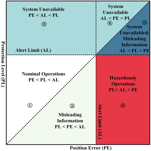
Figure 3. Stanford Diagram [12].

The RAIM algorithm should minimize the probability of events in region ③ to improve system availability; and minimize $P_{\text{MI}}$ and $P_{\text{HMI}}$ so that they do not exceed at least the preset IR to guarantee integrity.

2.2 Typical fault detection and exclusion method

RAIM usually requires fault detection, identification, and exclusion based on redundant measurement information. This subsection introduces several typical FDE methods to set the stage for the subsequent introduction of RAIM algorithms.

2.2.1 ${\mathit{\chi }}^{\mathbf{2}}$ test

The ${\chi }^2$ test [13], which is the most typical fault detection method, constructs the residual in the least squares (LS) algorithm or the innovation in the Kalman filter (KF) as a test statistic $t_k$, as shown in Equation 2:

$t_k={\mathit{r}}_k^T{\mathit{S}}_k^{-1}{\mathit{r}}_k(2)$

In the equation, ${\mathit{r}}_k$ is the residual or innovation, ${\mathit{S}}_k$ is its covariance matrix, and $k$ is the index of the measurement epoch, assuming that the measurement noise follows a zero-mean Gaussian distribution, $t_k$ will obey a central ${\chi }^2$ distribution under the fault-free hypothesis ${\mathcal{H}}_0$ (fault-free case), and a non-central ${\chi }^2$ distribution under the fault hypothesis ${\mathcal{H}}_1$ (faulty case), as shown in Equation 3:

$t_k\sim \left\{\begin{array}{l}{\chi }^2\left(df\right){\mathcal{H}}_0\\ {\chi }^2\left(df,\lambda \right){\mathcal{H}}_1\end{array}\right.(3)$

where $df$ is the degree of freedom of the ${\chi }^2$ distribution, depending on the number of visible satellites, and $\lambda$ is the non-centrality parameter.

When $t_k$ is greater than the detection threshold $T_k$, the fault hypothesis ${\mathcal{H}}_1$ is accepted to alert the user, and vice versa, the fault-free hypothesis ${\mathcal{H}}_0$ is accepted. The false alarm rate $P_{\text{FA}}$ and the missed detection rate $P_{\text{MD}}$ are usually set according to the application requirements, and their relationship with $T_k$ is shown in Figure 4.

Figure 4

Figure 4. Principle of the ${\chi }^2$ test.

After a fault is detected by the ${\chi }^2$ test, the fault can be further identified by the subset ${\chi }^2$ test [14], a method that recalculates the test statistic by removing one satellite measurements in turn, and ultimately selects the set of satellite measurements that passes the ${\chi }^2$ test with the smallest test statistic.

2.2.2 W-test

The w-test [15, 16] implements the FDE by performing a mean-shifted Gaussian test on each component of the normalized residual or innovation, and its test statistic is calculated as shown in Equation 4:

$w_k^{\left(i\right)}=\left|\frac{r_k^{\left(i\right)}}{\sqrt{{\mathit{S}}_k^{\left(i,i\right)}}}\right|(4)$

where $r_k^{\left(i\right)}$ is the $i$-th component in the residual or innovation ${\mathit{r}}_k$, and $S_k^{\left(i,i\right)}$ is the $i$-th diagonal element in its covariance matrix ${\mathit{S}}_k$. If $w_k^{\left(i\right)}$ exceeds the detection threshold $N_{1-P_{\text{FA}}/2}\left(0,1\right)$, the $i$-th satellite measurement is considered to be possibly faulty, and after completing the test for all satellite measurements, the maximum value exceeding the detection threshold is usually considered faulty and excluded, after which the w-test is re-run to verify that no other faulty measurements still exist. Typically, the w-test is used for fault identification and exclusion when a fault is detected in the ${\chi }^2$ test.

2.2.3 Solution separation

The solution separation (SS) [17, 18] method is no longer carried out in the range domain but directly implements fault detection on the position domain and is able to synchronize fault identification and exclusion. The computation process of its test statistics is shown in Figure 5, It accepts the fault hypothesis ${\mathcal{H}}_i$ and excludes the corresponding fault measurement when the test statistic $d_k^{\left(i\right)}$ exceeds the corresponding detection threshold $D_k^{\left(i\right)}$.

Figure 5

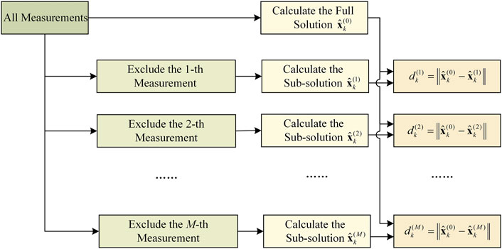
Figure 5. Calculation flowchart of the SS method.

2.2.4 Likelihood ratio test

The likelihood ratio test [11] is able to give the optimal result for hypothesis testing, using the ratio of the likelihood function of the measurement vector under opposing hypotheses to construct the test statistic, as shown in Equation 5:

$l_k=\mathit{ln}\left(\frac{p\left({\mathit{y}}_k\mid {\mathcal{H}}_m\right)}{p\left({\mathit{y}}_k\mid {\mathcal{H}}_0\right)}\right)(5)$

In the equation, $p\left({\mathit{y}}_k\mid {\mathcal{H}}_0\right)$ is the likelihood function under the fault-free hypothesis ${\mathcal{H}}_0$, and $p\left({\mathit{y}}_k\mid {\mathcal{H}}_m\right)$ is the likelihood function under the fault hypothesis ${\mathcal{H}}_m$. In practical RAIM applications, $p\left({\mathit{y}}_k\mid {\mathcal{H}}_m\right)$ is usually computed after excluding the measurement under the corresponding fault hypothesis [19, 20], and this approach is similar to the SS method, which can also be synchronized to achieve FDE.

3 RAIM algorithms

RAIM algorithm usually consists of two modules: the FDE module and the error bounding module. The FDE module detects, identifies and excludes faulty measurements based on the consistency checking principle using redundant measurement information. For a single-constellation receiver, at least five visible satellites are required to perform fault detection, and at least six visible satellites are required to perform fault exclusion [6]. The error bounding module is usually realized by calculating the PL, which is calculated by the user according to the requirements of the IR and other parameters, and compared with the preset al to discriminate the availability of the navigation system in real time. Currently, there are two main ways of calculating PL, one is to quantify the PE caused by undetected faults in the FDE module, and the other is to try to directly characterize the PE and then calculate its statistical bounds. Figure 6 provides a typical flow of RAIM, and it should be noted that not all RAIM algorithms strictly follow this general flow, and some algorithms may include additional steps or omit specific steps.

Figure 6

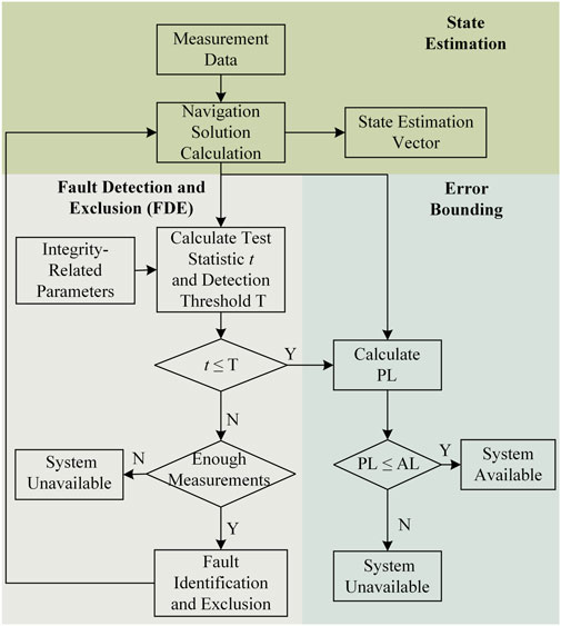
Figure 6. General RAIM algorithm flow [10].

Initially, traditional RAIM algorithms relied on prior modeling of the probability distribution of measurement errors or state estimation errors, which in turn led to the derivation of the probability distribution model of the test statistic for constructing hypothesis tests and calculating PL. However, since error probability distribution models are often difficult to build and validate accurately, the performance of RAIM based on these models is limited by the accuracy of the models, while RAIM based on set representation sidesteps this challenge by no longer treating errors as random quantities, but as unknown deterministic values. In addition, the data-driven ML approach provides another way of thinking for integrity monitoring, showing great potential and advantages in complex scenarios that are difficult to handle with traditional RAIM.

3.1 RAIM based on error probability distribution model

RAIM based on the error probability distribution model is the most widely used, which has the advantages of clear mathematical expression and the detection threshold can be calculated by the preset $P_{\text{FA}}$. Many studies have further divided the RAIM into snapshot scheme and filtering scheme, according to the number of measurement epochs used. The snapshot scheme is based on the current single-epoch measurement data only, and usually employs the LS algorithm for navigation solution calculation; The filtering scheme is based on current and historical measurement data, and usually employs the filtering methods such as the KF, extended KF (EKF), unscented KF (UKF) and the particle filter (PF), among other estimation methods for navigation solution calculation.

3.1.1 Classic LS RAIM

The classic LS RAIM is one of the most typical snapshot schemes. It models the pseudo-range error as a zero-mean Gaussian distribution in the fault-free case, introduces a mean deviation for the error distribution in the faulty case, and considers only the single fault case. The classic LS RAIM includes the pseudo-range comparison method [21], the least squares residual method [22], and the parity vector method [23]. The equivalence of these methods was theoretically demonstrated by [24], where the parity vector method employs an orthogonal transformation to convert residual vectors into parity vectors, providing computational simplicity and high efficiency in calculating test statistics [25].

In the FDE module, the classic LS RAIM employs the ${\chi }^2$ test for fault detection, which constructs the normalized sum of squares of the pseudo-range residual vectors as a test statistic as shown in Equation 2; after a fault has been detected, the w-test is usually used to further identify and exclude fault.

In the error bounding module, Brown et al [26] pioneered the approximated radial protection (ARP) algorithm for calculating the PL, whose computational principle is shown in Figure 7 [13]; if the measurement noise is ignored, there is a linear relationship between the test statistic $t$ and the horizontal PE (HPE), and different satellites $i$ have their own characteristic slope ${\text{SLOPE}}_i$ [27], assuming that the HPE caused by the failure of a single satellite is certain, the corresponding test statistic t is the smallest when the failure occurs on the satellite with the largest characteristic slope ${\text{SLOPE}}_{\mathrm{MAX}}$, making the failure most difficult to be detected. Based on this assumption, the calculation method of HPL is given as shown in Equations 6, 7:

$\text{HPL}=\text{SLOP}{\mathrm{E}}_{\text{MAX}}·\sqrt{{\lambda }_{\mathit{min}}}·\sigma (6)$

$P_{\text{MD}}={\displaystyle \underset{0}{\overset{T_k}{\int }}}{f}_{{\chi }^2\left(n-4,{\lambda }_{\mathit{min}}\right)}\left(x\right)dx(7)$

Figure 7

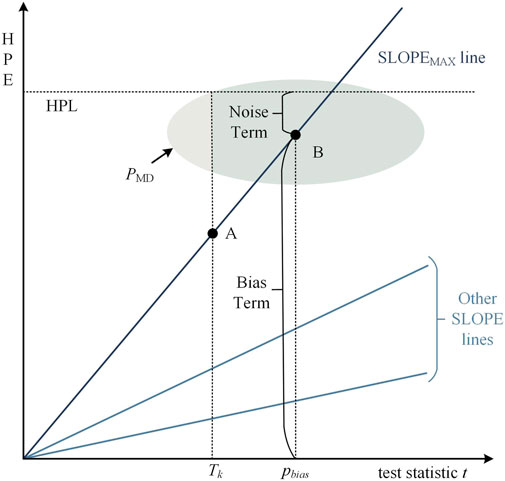
Figure 7. Principle of PL calculation in classic LS RAIM [13].

In the equation, $\sigma$ is the standard deviation of the measurement noise, and ${\lambda }_{\mathit{min}}$ is the minimum non-centrality parameter required to satisfy the specified $P_{\text{FA}}$ and $P_{\text{MD}}$. This parameter can be can be calculated according to Equation 7, where $n$ is the number of visible satellites.

Since the ARP algorithm ignores the effect of measurement noise, in this regard, Sang and Kubik [28] proposed an improved ARP algorithm by incorporating a term related to measurement noise to the PL calculation. The calculation principle is also shown in Figure 7 [13], when the measurement noise is ignored, the minimum detectable fault corresponds to point A in the figure, when the measurement noise is taken into account, the distribution of the test statistic t and the HPE will be elliptical, and the center of the ellipse corresponds to point B in the figure. The HPL is thus divided into bias term and noise term, as shown in Equations 8, 9. The bias term is calculated using the typical ARP algorithm, and the noise term is calculated by multiplying the expansion factor $k$ and the standard deviation ${\sigma }_H$ of the HPE, which is borrowed from the kSigma algorithm commonly used in the monitoring of system-level integrity [29].

$\text{HPL}=\text{SLOP}{\mathrm{E}}_{\text{MAX}}·p_{bias}+k·{\sigma }_H(8)$

$p_{bias}=\sqrt{{\lambda }_{\mathit{min}}}·\sigma (9)$

In the equation, $k$ is the expansion factor related to $P_{\text{MD}}$, and $\sigma$ is the standard deviation of the measurement noise.

3.1.2 Advanced RAIM and relative RAIM

Classic LS RAIM is unable to meet the high integrity requirements of the precision approach phase of civil aviation. In response, the GNSS Evolutionary Architecture Study (GEAS) Panel developed advanced RAIM (ARAIM) algorithm [30–34]. Compared with the classic LS RAIM algorithm, ARAIM has several advantages, including the ability to detect and recognize multi-faults, applicability to multi-constellation GNSS, the ability to monitor integrity in the vertical direction, and the capability to eliminate the first-order ionospheric delay using dual-frequency measurements.

ARAIM employs the Multiple Hypothesis Solution Separation (MHSS) [35, 36] algorithm for FDE, which allows for multi-faults detection by additionally considering multi-faults scenarios on top of the traditional SS method. In addition, ARAIM assigns a specific $P_{\text{FA}}$ and $P_{\text{HMI}}$ values to each fault hypothesis, performs independent hypothesis testing and PL computation, and assigns a specific $P_{\text{HMI}}$ to the fault-free hypothesis ${\mathcal{H}}_0$ for the computation of PL in the case of fault-free. Ultimately, it takes the maximum value as the final PL. The detailed algorithm of ARAIM can be found in [37].

The ARAIM algorithm relies on periodically received integrity support messages (ISM) [38]. To guarantee integrity over longer reception intervals, relative RAIM (RRAIM) has been proposed [30, 39]. The RRAIM algorithm employs a time-differenced carrier phase measurement, defining the epoch of the received ISM as the initial time, and defines the interval from the current epoch back to the initial time as the coasting time. The algorithm combines the pseudo-range of the initial time and the variation of the carrier phase within the coasting time to construct a new measurement model, which employs a residual-based χ² test for fault detection. Similar to ARAIM, PL is calculated under each hypothesis separately, and the maximum of all results is taken as the final PL [40]. pointed out that system availability is closely related to the length of the coasting time, with the best availability achieved when the coasting time is around 1 min; after this, availability gradually decreases with the extension of the coasting time.

So far, there are still ongoing research efforts aimed at improving to the ARAIM algorithm to improve its performance, and these improvements are mainly focused on the following four aspects:

1) When the number of visible satellites is large and the maximum number of faults (the hypothesis that the number of faults is greater than this value is ignored) is large, the computational burden of ARAIM increases significantly, so there are researches aiming to improve its computational efficiency.

2) The traditional ARAIM algorithm assigns $P_{\text{FA}}$ and $P_{\text{HMI}}$ fixed to each fault hypothesis ${\mathcal{H}}_i$, and simply averages them for the same type of fault hypotheses, in this regard, some studies have proposed to optimize the allocation of $P_{\text{FA}}$ and $P_{\text{HMI}}$ to improve the availability.

3) ARAIM also models the measurement errors as Gaussian distributions and obtains parameters such as the mean and variance of the error model based on the ISM parameters, and some studies aim to improve the performance of ARAIM by accurately calculating the model parameters or improving the error model.

4) The traditional ARAIM is based on pseudo-range only, in view of the high accuracy advantage of carrier phase, some studies have adopted carrier phase measurement on the basis of ARAIM framework.

This paper summarizes the latest ARAIM improvement studies in the above four aspects as shown in Table 1.

Table 1

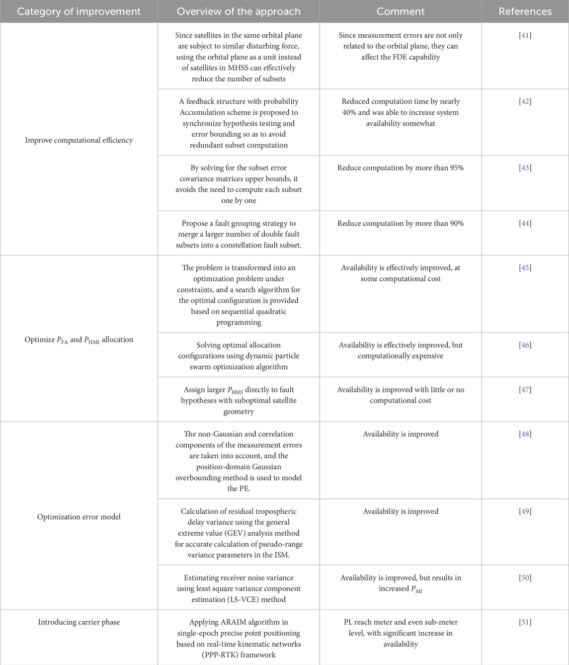
Table 1. Status of ARAIM improvement research.

3.1.3 KF-based RAIM

The above two types of methods belong to the category of snapshot scheme, which only uses single-epoch measurements, and can quickly detect step errors, but the detection ability of slowly growing errors (SGEs) is seriously insufficient; in addition, they are only applicable to receivers that use the LS algorithm for navigation solving, and can not be applied to the real time kinematic (RTK) or precise point positioning (PPP) receivers that have to use filtering methods such as KF. The KF-based RAIM (KF-RAIM) algorithm introduced next can well solve the above problems. Traditional KF-RAIM borrows from the classic LS RAIM and employs residuals or innovations for FDE, such as autonomous integrity monitoring by extrapolation (AIME) [52, 53], extended RAIM (ERAIM) [54, 55], and other typical algorithms. AIME constructs the normalized sum of squares of the innovations ${\mathit{r}}_k$ as the test statistic $s_k^2$, and to improve the detection of SGEs, performs a weighted average within a sliding time window, as shown in Equations 10–12:

$s_k^2=\left({\mathit{r}}_{avg}^T\right)\left({\mathit{S}}_{avg}^{-1}\right)\left({\mathit{r}}_{avg}\right)(10)$

${\mathit{r}}_{avg}={\left({\mathit{S}}_{avg}^{-1}\right)}^{-1}{\displaystyle \sum _{j=k-\tau +1}^k}{\mathit{S}}_j^{-1}{\mathit{r}}_j(11)$

${\mathit{S}}_{avg}^{-1}={\displaystyle \sum _{j=k-\tau +1}^k}{\mathit{S}}_j^{-1}(12)$

where $\tau$ is the time window length, ${\mathit{r}}_j$ is the innovation, and ${\mathit{S}}_j$ is its covariance matrix. The detection delay of the AIME algorithm for the SGEs is inversely proportional to its growth rate, in order to further reduce the detection delay, Bhatti and Ochieng [56] proposed a rate detection method, which adds a KF based on the AIME algorithm to monitor the rate of change of $s_k^2$, reducing the SGEs detection delay by more than 33%.The ERAIM algorithm [54, 55], on the other hand, combines the predicted state vectors and measurement vectors in the KF, constructs a new measurement model and calculates the residuals, which in turn is used for the FDE using the ${\chi }^2$ test and the w-test. In addition, the correlation coefficients between the test statistics are also calculated by ERAIM, which is used to analyze the separability of the faults.

Carrier phase measurements are usually several orders of magnitude more accurate and more robust to noise compared to code measurements. Therefore, Feng et al. [57] developed carrier phase-based RAIM (CRAIM) using innovations to guarantee the integrity of relative positioning, and Schuster et al. [58] further utilized CRAIM for RTK positioning. The CRAIM algorithm uses the double difference of pseudo-range, wide lane, and carrier phase measurements as the EKF measurements, estimating the ambiguity of whole cycles as states to assist in ambiguity resolution. In addition, CRAIM can use the carrier phase measurements to construct a specialized test statistic for detecting cycle slip faults. Addressing the lack of fault identification capability in the CRAIM algorithm, Liu et al. [59] further proposed an extended w-test method with multi-fault detection and identification capability.

In addition to the KF-RAIM based on residuals or innovations, the KF-RAIM based on SS is also widely used [17]. Its test statistics are computed as shown in Figure 4, featuring the unique capability of using both main filter and sub-filters to compute the full solution ${\widehat{\mathit{x}}}_k^{\left(0\right)}$ and sub-solution ${\widehat{\mathit{x}}}_k^{\left(i\right)}$ in parallel. However, the method proposed in [17] lacks multi-fault detection capability and cannot detect INS fault in GNSS/INS integrated navigation. To address this problem, Bhatti et al. [60] proposed a FDE method using a multi-stage parallel subset filter based on the MHSS, which can detect and identify double faults, including INS fault. Zhang et al. [61] further improved the filter bank scheme so that it can be applied to carrier phases for integrity monitoring in PPP, and noting that periodic initialization of the filters can reduce the maximum number of faults that need to be considered, thereby effectively reducing the computational burden. Meng et al. [62], instead of adopting the filter bank scheme, consider the new measurement model constructed in ERAIM as a “pseudo-snapshot” model, and then use the least squares form of the SS method to compute the full solution ${\widehat{\mathit{x}}}_k^{\left(0\right)}$ and the sub-solution ${\widehat{\mathit{x}}}_k^{\left(i\right)}$, which reduces the computational burden to some extent. Gao et al [63] further applied this method to integrity monitoring in RTK positioning and used it to detect fault ambiguity solution.

In terms of error bounding, the innovation or residual-based KF-RAIM divides the PL into a noise term and a bias term [64], where the noise term represents the upper bound of the PE caused by the noise, and the bias term represents the upper bound of the PE caused by measurement bias. In contrast, the SS-based KF-RAIM directly takes the detection threshold $D_k^{\left(i\right)}$ in each fault hypothesis ${\mathcal{H}}_i$ as a bias term, as shown in Equation 13:

${PL}_k=\underset{i}{\mathit{max}}\left\{a_k^{\left(i\right)}+D_k^{\left(i\right)}\right\}(13)$

where the noise term $a_k^{\left(i\right)}$ can be solved based on $P_{\text{MD}}$ and the state covariance matrix of each sub-filter. Tanil et al. [65] compared the above two types of methods in GNSS/INS integrated navigation in an urban environment, and the results showed that when the number of visible satellites is more than four, the KF-RAIM based on the SS method has a smaller $P_{\text{HMI}}$, but the computational burden is heavier.

In view of the high accuracy of carrier phase measurements, the PL calculated by KF-RAIM with the introduction of carrier phase is significantly smaller, reaching meter or even sub-meter level. This improvement enhances the availability of the system, and the experimental results of Schuster et al. [58] show that the HPL calculated by the CRAIM algorithm is in the range of 0.5 m in the case of fault-free. In addition, since carrier phase measurements usually require a ratio test [66] to verify whether the ambiguity of whole cycles is correctly fixed, Li et al. [67] introduced the concept of completeness to the ambiguity validation by defining an ambiguity protection level. When the ambiguity protection level exceeds the ambiguity alarm threshold, the ambiguity validation is considered to have failed, and an alarm is generated.

Since KF and EKF are always limited by Gaussian error models, the actual measurement error and state estimation error are affected by various factors such as receiver motion, linearization modeling errors of nonlinear models, and residual tropospheric and ionospheric errors. As a result, the Gaussian assumption is not appropriate, leading to inherent limitations in KF-RAIM [68]. In response to this challenge, some studies have begun to explore KF-RAIM based on non-Gaussian error models.

Madrid et al. [69] proposed an integrity monitoring scheme called Kalman integrated protection level (KIPL) based on the isotropy assumption (the residual vector points in any direction with equal probability over the measurement space) [70]. The approach models the measurement error as a Student’s t-distribution, which in turn leads to the derivation of a Student’s t-distribution model for the state estimation error, which ultimately allows for the computation of the PL based on the preset IR. Validation results from Gottschalg et al. [71] show that the HPL calculated by KIPL is smaller compared to that calculated by traditional KF-RAIM under the same IR requirement. Wang et al. [72] further extended this algorithm for application in PPP. Similarly, Shao et al. [68] used a robust KF based on the Student’s t distribution [73] for state estimation, which models both measurement and process noises as student’s t-distributions. This method uses a variational Bayesian approach to approximate the state estimation error as a Gaussian distribution for calculating the PL [68]. also discusses multi-faults detection and identification schemes accordingly.

3.1.4 PF-based RAIM

PF allows better state estimation in nonlinear systems and non-Gaussian noise conditions, eliminating the Gaussian noise assumption restriction found in traditional KF-RAIM. Moreover, the posteriori particle ensemble of PF provides a new approach for error bounding.

Li and Kadirkamanathan [74] were the first to propose the introduction of the likelihood ratio test in PF to achieve fault detection. Based on this, some studies [20, 75, 76] borrowed the concept of the SS method and used the likelihood ratio test for integrity monitoring by constructing a parallel filter bank. They calculated the cumulative log-likelihood ratio $LL{R}_k^{\left(i\right)}$ in the time window under different fault hypothesis ${\mathcal{H}}_i$ as a test statistic, as shown in Equation 14:

$LL{R}_k^{\left(i\right)}={\displaystyle \sum _{j=k-\tau +1}^k}\mathit{ln}\left(\frac{{\displaystyle {\sum }_{r=1}^N}p\left({\mathit{z}}_j|{\mathit{x}}_j^{\left(i\right)}\left(r\right)\right)}{{\displaystyle {\sum }_{r=1}^N}p\left({\mathit{z}}_j|{\mathit{x}}_j^{\left(0\right)}\left(r\right)\right)}\right)(14)$

where $\tau$ is the time window length, $k$ denotes the current epoch, $i$ is the fault hypothesis index, $r$ is the particle index, $N$ is the total number of particles, $p\left({\mathit{z}}_j|{\mathit{x}}_j^{\left(i\right)}\left(r\right)\right)$ and $p\left({\mathit{z}}_j|{\mathit{x}}_j^{\left(0\right)}\left(r\right)\right)$ are the likelihood functions under the fault hypothesis ${\mathcal{H}}_i$ and the fault-free hypothesis ${\mathcal{H}}_0$, respectively. The maximum value of $LL{R}_k^{\left(i\right)}$ is usually taken as the test statistic. The fault detection threshold of this method typically needs to be selected empirically, for this problem, He et al [77] proposed to optimize the computation of the detection threshold using a genetic algorithm.

The above fault detection methods require several parallel PFs, which can impose a significant computational burden in the case of a large number of visible satellites. To address this, Han et al. [78] proposed constructing the test statistic using the measurement residuals vector corresponding to the particle of maximum weight, pointing out that the correlation between the residual vector and the satellite projection vector can be used to identify faulty satellites. Hafez et al. [79] proposed constructing the test statistic using the weighted average measurement predicted value of the particle ensemble.

The error bounding method of PF-RAIM is more special, evaluating the actual IR based on the a posteriori set of particles to achieve error bounding, known as Bayesian RAIM (BRAIM) [80]. BRAIM calculates the error of each particle state with respect to the a posteriori estimation and accumulates the weights of the particles whose errors exceed the AL to obtain the estimated integrity risk. This risk is then compared with the preset IR to determine availability, as illustrated in Figure 8 [81]. Gabela et al. [82, 83] further improved this scheme by introducing spatial feature constraint information to assist the weight update step in PF. Empirical results show that with the HAL set to 5 m and the IR requirement specified, the navigation system’s availability exceeds 99%, regardless of whether the measurement noise is modeled as a Gaussian model or a three-component Gaussian mixture model (GMM).

Figure 8

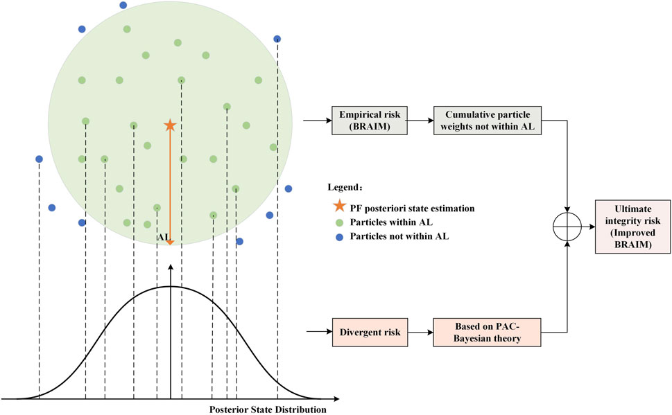
Figure 8. Braim and improved BRAIM Schematics [81].

However, the integrity risk estimated by BRAIM is only the empirical risk based on the set of particles, which has limitations. Because the number of particles in the PF is always limited, it does not fully reflect the state posterior distribution, leading to some underestimation of the estimated integrity risk. Regarding this problem, Gupta et al [81, 84] proposed an improved BRAIM algorithm based on probably approximately correct- Bayesian (PAC-Bayesian) theory, which introduces the divergence risk to quantify the uncertainty caused by the above problem, and derives a method for calculating the upper bound on IR, which is also schematically shown in Figure 8 [81]. Additionally, this study models the measurement noise as a GMM while employing the expectation-maximization (EM) algorithm to determine the model parameters, thereby reducing the difficulty of model parameter estimation.

On the other hand, the particle impoverishment problem, i.e., reduced particle diversity, arises from the resampling operation in PF, which affects the performance of PF-RAIM. In this regard, several studies have proposed improvements to address particle impoverishment, including: introducing a Markov chain Monte Carlo (MCMC) moving step for each particle [75, 85], utilizing selection, crossover, and mutation operations in genetic algorithms to replace the traditional resampling method [86], employing backpropagation neural network (BPNN) to adjust the particle weights [87], and using chaotic particle swarm optimization algorithms to increase particle diversity [20].

3.1.5 Brief summary

Table 2 provides a comparative analysis of different RAIM algorithms based on the error probability distribution model. Among them, the snapshot scheme can quickly detect step errors; however, due to its reliance on only a single epoch measurement, its detection capability is seriously insufficient for SGEs caused by aging satellite equipment or clock drift. In this regard, some studies [88, 89] have improved the snapshot scheme by averaging the test statistics within a sliding time window to enhance SGEs detection capability. Additionally, the filtering scheme can be easily integrated with the INS, and the additional redundant information provided by the INS can effectively improve the system’s availability. However, the introduction of the INS also brings an additional source of integrity risk.

Table 2

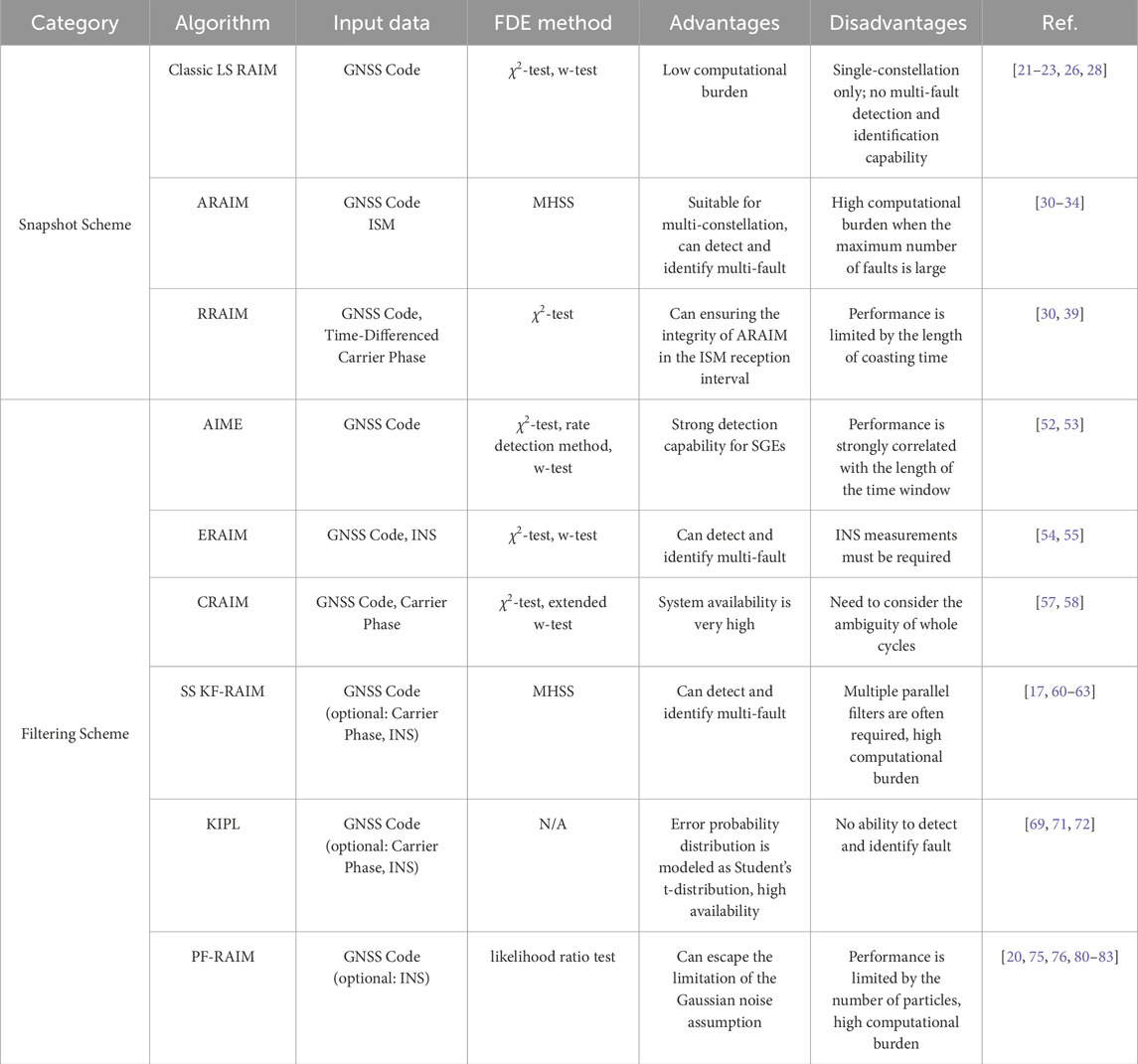
Table 2. Comparative Analysis of RAIM based on error probability distribution model.

3.2 RAIM based on set representation

Traditional RAIM always assumes that the error probability distribution model is known, but in practice, there are significant challenges in the accurate construction and validation of the error probability distribution model. RAIM based on set representation is able to get rid of the limitation of traditional statistical distribution models, and this type of approach treats the error as an unknown deterministic value, aiming to construct the set characterizing the state estimation error by determining the uncertainty intervals of the error, which is used for further FDE and error bounding.

3.2.1 FDE module

In the FDE module [90], proposes an innovative fault detection strategy based on set representation theory, converts the navigation problem into a convex polytope solving problem by applying the uncertainty interval $\left[-\mathit{e},\mathit{e}\right]$ of the observation error to the observed-minus-computed values (OMC) vector $\mathit{y}$ as shown in Equation 15.

$\mathit{y}-\mathit{e}\le \mathit{A}\delta \mathit{x}\le \mathit{y}+\mathit{e}(15)$

In the above equation, $\mathit{A}$ is the design matrix and $\delta \mathit{x}$ is the state estimation vector. It has been shown that the volume of the polytope is negatively correlated with the degree of consistency of the measurements, therefore, a decrease in the volume predicts an increase in the probability of the existence of fault measurements, which in turn leads to the proposal of a new inconsistency metric that warns the user when it exceeds a threshold value. In addition, when the fault value is large, the polytope will be the empty set, so some studies also directly achieve fault detection by determining whether the set of polytope characterizing the state estimation error is empty [91, 92], it is worth noting that [91] compares this method with the traditional classical LS RAIM and ARAIM algorithms based on the SS method, under the assumption of Gaussian noise were compared, but found to be inferior to the traditional methods in terms of fault detection rate and $P_{\text{HMI}}$ metrics [92]. further proposed a corresponding fault identification and exclusion scheme based on the SS idea on the basis of this method.

3.2.2 Error bounding module

The advantage of RAIM based on set representation is reflected in the error bounding module, which can compute the set characterizing the state estimation errors in real time. Among many studies, a special polytope, namely, the zonotope, has been widely chosen as a set representation of the state estimation errors due to its favorable mathematical properties (e.g., Minkowski sum, linear transformation) [93]. The zonotope $\mathbb{Z}$ was first used by Combastel [94] to characterize the state estimation errors $\mathrm{\delta }\mathbf{x}$, which is defined as:

$\mathbb{Z}=<\mathbf{c},\mathbf{H}>=\left\{\mathrm{\delta }\mathbf{x}\in {\mathbb{R}}^n\mid \mathrm{\delta }\mathbf{x}=\mathbf{c}+\mathbf{\text{Hb}}|{‖\mathbf{b}‖}_{\infty }\le 1\right\}(16)$

in Equation 16, $\mathbf{c}\in {\mathbb{R}}^n$ is called the center vector, $\mathbf{H}\in {\mathbb{R}}^{n\times m}$ is called the generation matrix, and $m$ is the order of the zonotope $\mathbb{Z}$. By adjusting the order $m$, the number of faces and the shape of $\mathbb{Z}$ can be changed, making it more flexible in characterizing the state estimation errors. Usually, zonotope is used in combination with filter estimation methods. Liu et al. [93] used zonotope for error bounding and PL calculation in tightly coupled GNSS/INS navigation systems, and pioneered the use of the extended H-infinity filter (EHF), which treats the noise as an unknown deterministic quantity instead of a random quantity, to replace the traditional EKF for state estimation. And the validation results show that the proposed method has higher system availability and lower $P_{\text{MI}}$ than the traditional KF-RAIM.

Referring to the [93, 95], this paper summarizes the generalized flowchart of error bounding based on zonotope set representation at the $k$-th epoch in Figure 9. It is worth noting that, as epoch $k$ advances, the order of the zonotope set characterizing the state estimation error will increase, which will generate a huge computational burden and affect the real-time performance of the algorithm, in this regard [93], proposes an order limitation scheme based on the zonotope reduction method, with the upper limit of the order being customized by the user, and experimentally explores the effect of the order on the computational time and PL.

Figure 9

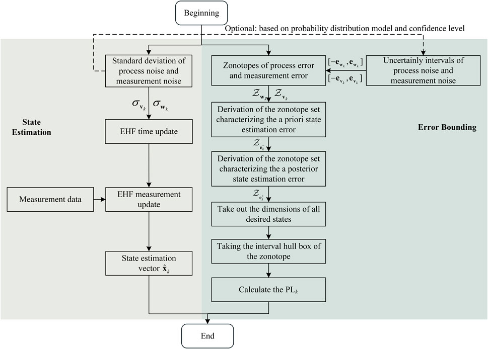
Figure 9. Generalized flowchart of error bounding based on zonotope set representation.

In addition to the above studies using the standard zonotope set, there have been some studies using variants of the zonotope for error bounding. Ashraf et al. [95] proposed to use constrained zonotope to characterize the state estimation error, which makes the geometry of the set more closely match the actual state space and further reduces the conservatism of error bounding. Shetty et al. [96], on the other hand, chose to adopt probabilistic zonotopes as a set representation tool while still assuming that the measurement errors and process errors follow a Gaussian distribution. This allows the state estimation error set to be solved according to the preset confidence level; however, there are some limitations, as the Gaussian distribution assumption is not strictly valid. Additionally [96], employs urban 3D maps and ray-tracing to determine multipath errors uncertainty intervals, in turn, the uncertainty interval of the measurement errors is determined. Su et al [92, 97], on the other hand, proposed an extended point confidence region for characterizing the state-domain error set, which uses a zonotope set to quantify the impact caused by systematic errors, and at the same time uses the traditional confidence ellipsoid or ellipsoid set to quantify the impact caused by stochastic errors, and finally take the Minkowski sum of the two sets as the final set of state estimation errors.

3.2.3 Brief summary

At present, there are not many studies on RAIM based on set representation. Theoretically, this approach does not rely on the error probability distribution model; however, many studies still use the traditional Gaussian distribution assumption to determine the error uncertainty interval based on the preset confidence level. Only some studies have discussed the determination of measurement error intervals, such as those for multipath errors [92, 96] and residual tropospheric and ionospheric errors [98]. These studies cover only part of the measurement errors and lack the determination of process error intervals. There have been studies using ML methods to estimate pseudo-range errors [99, 100], suggesting that attempts could be made to predict the uncertainty intervals of pseudo-range errors with the help of ML, which may be a direction for further research in the future.

3.3 ML-based RAIM

ML-based RAIM (ML-RAIM) has great potential and advantages, as it can effectively address the challenges posed by nonlinear systems and non-Gaussian noise, and it supports integrity monitoring in complex scenarios where it is difficult to model error probability distributions in traditional RAIM (e.g., urban canyon). In addition, since ML-RAIM mostly follow the idea of characterizing the PE in calculating the PL, it makes the two modules of FDE and error bounding relatively independent of the study.

3.3.1 FDE module

According to whether the training data need labels, ML algorithms can be classified into two main categories: supervised learning and unsupervised learning. Supervised learning relies on labeled datasets for training, while unsupervised learning does not require data labels.

In terms of supervised learning research, it can be categorized as traditional pattern recognition, traditional neural networks, and deep learning based on the ML algorithms employed in the research. Traditional pattern recognition methods with inherent advantages such as high interpretability and fast training speed are widely used to detect and identify faulty measurements, especially for NLOS signals [101]. used support vector machine (SVM) algorithm to classify LOS signals and NLOS signals, and six commonly used features were analyzed, and it was found that the feature of pseudo-range residuals had no significant contribution [102]. systematically evaluated the detection effectiveness of various ML algorithms under different fault thresholds and found that the k-nearest neighbor (KNN) algorithm exhibits an optimal fault detection rate.

Compared to single models, ensemble learning has good robustness and stability by combining the prediction results of multiple base learners. Comparative studies in [103] have shown that boosting and bagging ensemble learning algorithms exhibit better performance in NLOS signal detection compared to single models such as support vector regression (SVR), KNN and gradient boosting decision tree (GBDT). Among them, the random forest (RF) algorithm with Bagging strategy performs most prominently. Based on RF algorithm [104], used factor analysis to aggregate the original features into three more interpretable common factors, which improved computational efficiency by about 30%. While the base learner of the above two types of ensemble learning is limited to the same class of models [105], innovatively detects NLOS signals based on the stacking ensemble learning (SEL) algorithm, which supports the use of different classes of models as the base learner. It achieves better generalization ability in different scenarios such as static, low-speed, and high-speed dynamic.

Many studies have also used traditional neural network (NN) algorithms with relatively simple structures for FDE [106]. directly predicts the receiver fault rate based on multi-layer perceptron (MLP) algorithm and alerts the user when the prediction exceeds a specified threshold [107], proposes a NLOS signal detection scheme based on the MLP algorithm, which effectively improves the PPP-RTK positioning accuracy.

Among the traditional NN algorithms, radial basis function neural network (RBFNN) has received a lot of attention from researchers due to its fast training speed and applicability to small sample datasets. Zheng et al. [108] used probabilistic neural network (PNN), which is an RBFNN integrated with Bayesian theory, to propose a fault detection scheme that employs a particle swarm optimization algorithm to compute a specific fitness function, ensuring the preset $P_{\text{FA}}$ and $P_{\text{MD}}$ [108]. also proposed a novel dataset acquisition method to generate training data by sampling the position error distribution in fault and fault-free modes according to the variance inflation model. Huang et al. [109] also used a similar method to acquire training data, employing nonparametric estimation-based neural network (NE-NN) for fault detection and combining it with the SS method for fault identification. Wu et al. [110] similarly proposed a PNN-based fault detection and identification method characterized by the use of single-satellite multi-epoch pseudo-range residuals as feature vectors, which has higher sensitivity compared to classic LS RAIM.

Deep learning algorithms consist of multi-layer NNs that can automatically learn and extract higher-order features from the data and have high generalization ability. Zhu et al [111] enriched and enhanced one-dimensional features within a time window into two-dimensional features and proposed an NLOS signal detection scheme based on convolutional neural network (CNN). Sun et al [112] used a long short-term memory (LSTM) for fault detection, and specially designed a loss function to synthesize the advantages of the snapshot scheme and the filtering scheme, thus improving the detection performance for small magnitude step errors and SGEs [113]. used Hopfield network for NLOS signals detection, and the experimental results show that accuracy is effectively improved compared with traditional SVM and gradient boost machine (GBM) algorithms.

In addition, it has been found that the emergence of NLOS signals has obvious spatiotemporal correlation [114–116], and the self-attention mechanism is able to capture long-range dependence and global contextual information by calculating the relational weights between any two elements in the sequence. Therefore [116], proposed a dual self-attention mechanism (DSN) model to construct two self-attention channels to extract spatial environment features and signal time features, respectively; the former inputs the feature data of all measurements, while the latter inputs the historical feature data of the target measurement, which significantly improves the detection effect of NLOS signals.

On the other hand, in order to cope with the difficulty of adapting the trained model to new environments, and to further improve the model generalization ability [115], further introduced the Siamese neural network architecture based on DSN model, so that the model can be quickly adapted to new environments under the condition of few-shot labeled data. Similarly, Sun et al [117, 118] also proposed a continuous learning-based NLOS detection scheme based on LSTM model, and the experimental results show that the proposed method improves the NLOS signal detection rate by 5%–12% in new environments compared with the traditional model fine-tuning scheme. Table 3 summarizes the above supervised learning-based FDE studies for comparison.

Table 3

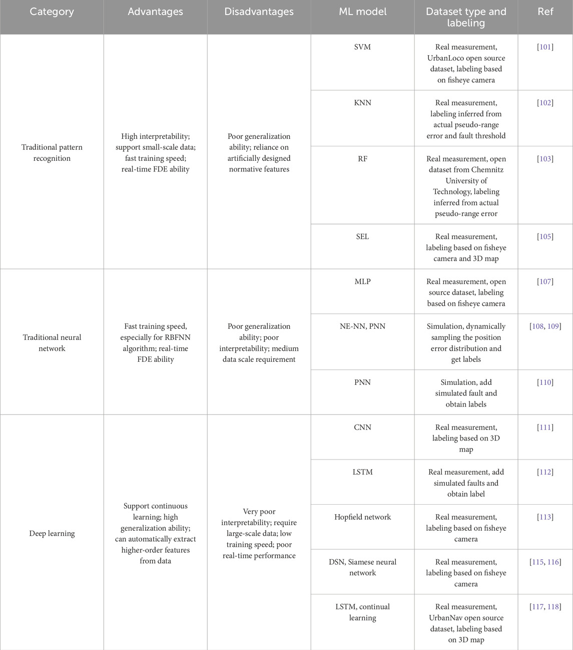
Table 3. FDE based on supervised learning.

Compared to supervised learning, FDE methods based on unsupervised learning do not rely on acquiring difficult labeled data and are able to cope with fault types that do not occur during training. The current research can be divided into two categories, one method is based on traditional clustering or single classification algorithms, and the other method is based on deep learning reconstructed models.

In the field of research based on traditional clustering or one-class classification algorithms, Xia et al [119] used the hierarchical density-based spatial clustering of applications with noise (HDBSCAN) algorithm to cluster and identify fault [120, 121]. compared three clustering algorithms, k-means, Gaussian mixed clustering and fuzzy c-means, and found that the k-means algorithm has the optimal performance in identifying NLOS signals. Wang et al. [122] proposed a fault detection scheme based on the one-class support vector machine (OCSVM) algorithm, which uses only the data from the fault-free case as the training dataset. A fault is detected when the similarity measure of the OCSVM outputs is less than a specified threshold.

Another type of fault detection principle based on deep learning reconstruction model is: using the data in the fault-free case to train the model with data reconstruction ability, when the difference between the model output and the real sample is too large, it indicates that there is a fault. Kim et al. [123] utilized a time-delayed neural network (TDNN) to make predictions based on historical test statistics and compared them with the current test statistics for fault detection. Gogliettino et al. [106] proposed an autoencoder-based fault detection scheme by calculating the difference between the input data and the reconstruction results from the autoencoder, determining that it is a faulty case when the difference exceeds a specified threshold. Shen et al. [124] proposed a combination of a generative adversarial network (GAN) and a recurrent neural network (RNN) for GNSS/INS integrated navigation integrity monitoring. The verification results show that the detection performance for small magnitude step errors and SGEs is improved compared to traditional KF-RAIM; however, this method assumes that the INS is always fault-free and ignores the potential fault risk of the INS. Table 4 summarizes the above unsupervised learning-based FDE studies for comparison.

Table 4

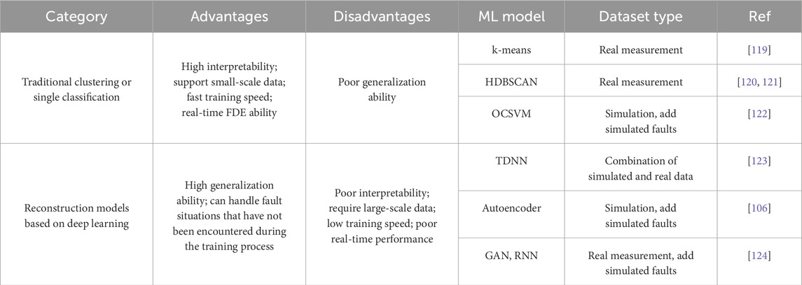
Table 4. FDE based on unsupervised learning.

3.3.2 Error bounding module

In terms of error bounding studies [109], borrowed the idea of PL calculation from the classical LS RAIM algorithm, i.e., to quantify the effect of undetected faults on PE, and proposed to calculate the maximum PE caused by undetected faults in the FDE module based on the search strategy, and then obtain the PL.

In addition, some studies have chosen to use ML algorithms to directly predict PL. Mendonca et al [125] proposed to use decision tree (DT) and NN algorithms to directly predict PL respectively, both of which have smaller $P_{\text{HMI}}$ compared to the traditional KF-RAIM. The conformal regression algorithm has the ability to output the confidence interval of the prediction result under the specified confidence level. Kuratomi et al [126] combined conformal regression with RF algorithm and proposed conformal regression forests (CRF) for predicting PE intervals at specified confidence levels, which provides insights for PL calculation. The confidence level was set to 99.999% in the paper, and the prediction is considered successful if the actual PE falls within the prediction interval. Unfortunately, the optimal set of experimental results in the paper only achieved a 99.99% prediction success rate, which requires further research.

Probabilistic regression ML algorithms provide the credibility or probability distribution model of the prediction results along with the output of the prediction results, so some researchers have tried to use probabilistic regression ML algorithms to predict the statistical characteristics of PE, thus realizing error bounding. Geragersian et al. [127] proposed the use of a Bayesian-LSTM algorithm to predict PE, and since the parameters of the Bayesian neural network are random quantities, the PE standard deviation can be estimated using Monte Carlo methods, and then obtain the PL. Isik et al. [128] proposed a scheme for PL calculation based on natural gradient boosting (NGBoost). The NGBoost algorithm is capable of predicting a probability distribution model that matches the input samples, but it requires pre-determination of the type of the probability distribution model. In this study, PE is assumed to be Gaussian distributed, and the mean and variance are predicted separately, which can be combined with a predefined confidence level to calculate the PL. The experimental results show that system availability is significantly improved in simulated suburban, urban, and urban canyon environments compared to classic LS RAIM. Table 5 summarizes and compares the above availability discriminative studies in ML-RAIM.

Table 5

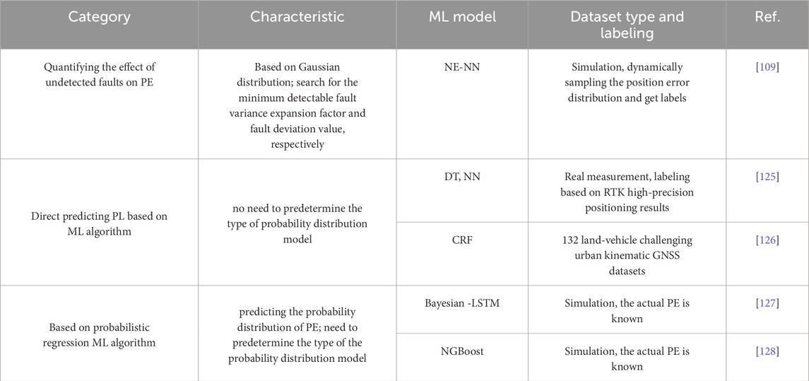
Table 5. ML-based error bounding studies.

3.3.3 Brief summary

Currently, there have been many ML-based GNSS jamming and spoofing detection studies [129–131], but relatively few studies have been applied to integrity monitoring. Although there are similarities between the two, the additional IR requirements of RAIM itself, along have made ML-RAIM studies relatively challenging. Firstly, the datasets used in existing studies are usually limited to a single scenario, failing to comprehensively reflect multiple factors such as satellite faults, ionospheric fluctuations, multipath effects, spoofing, and jamming. This results in flaws in the generalization ability of the trained models. Secondly, most current ML-based FDE strategies lack corresponding error bounding module studies, and in the few studies of error bounding, it is still limited to the traditional Gaussian distribution assumption. Thirdly, there is a lack of relevant research dedicated to feature extraction and selection.

3.4 Comparison and summary

The advantages and disadvantages of the above three types of RAIM algorithms are shown in Table 6.

Table 6

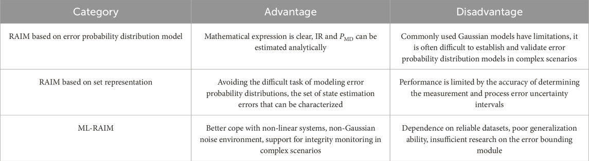
Table 6. Characteristics of the three types of RAIM.

4 Challenges and opportunities of RAIM research

With the wide application of GNSS, existing RAIM research faces the following challenges: Firstly, due to the vulnerability of the GNSS signals themselves, it is very susceptible to jamming and spoofing [132]. Additionally, for the vast number of urban users, multipath and even NLOS signals are very common, which leads RAIM to operate in a more complex and harsh electromagnetic environment. Secondly, in key applications such as assisted driving, autonomous driving, and low-altitude unmanned aerial vehicles (UAVs), the required PL is usually small, often in the meter or even sub-meter level [9]. However, the PL calculated by existing RAIM is often overly conservative (reaching up to tens of meters or even hundreds of meters), resulting in seriously inadequate system availability. Thirdly, most existing RAIM algorithms are based on the Gaussian error model, but the study by [133] have shown that actual measurement and position error often exhibit characteristics of heavy-tailed distributions, making the Gaussian assumption that do not hold strictly. In addition to considering the multipath effects, jamming and spoofing, etc., it is even more difficult for the actual error to follow the assumption of the Gaussian distribution, and at this time, if the Gaussian distribution is still used for modeling errors, an excessively large variance is required to ensure that the estimation of the error is conservative enough, thus seriously reducing the system availability [134].

Considering the current challenges and existing results, future opportunities for RAIM development lie in the following areas: the development and application of adaptive non-Gaussian error probability distributions; the application of more flexible and tight error bounding techniques; and the improvement of the ML-RAIM methods’ generalization ability.

4.1 Adaptive non-Gaussian error probability distributions

Firstly, there have been studies using student’s t-distribution [68] and GMM [84, 135] for modeling measurement or process errors and for integrity monitoring, with experimental results showing superior performance compared to traditional Gaussian model-based approaches. In addition, several other models have been employed to discuss error modeling, including the Rayleigh distribution and the generalized Pareto distribution (GPD) [136], the Dirichlet process mixture (DPM) model [137, 138], and the generalized extreme value (GEV) distribution [133]. Among these, the GPD and GEV distribution are based on extreme value theory and are specifically designed to analyze rare but potentially severe extreme events, focusing on the tail distribution properties of random variables. This aligns well with the needs of integrity studies and has been used for integrity risk assessment and validation [139]. The use of these non-Gaussian error models in conjunction with non-Gaussian noise estimators, such as PF, is expected to effectively improve integrity monitoring performance.

Secondly, almost all existing RAIM systems ignore the temporal correlation of measurement noise. However, colored noise is unavoidable and cannot be overlooked due to hardware noise, multipath effects, and unmodeled errors [140]. Gao et al. [141, 142] exploited the temporal correlation of colored noise by modeling it as a first-order Gaussian-Markov process. The proposed colored Kalman filter outperforms the traditional KF-RAIM in integrity monitoring. Therefore, studying and utilizing the temporal correlation of errors for error modeling will be an important opportunity for the future development of RAIM.

Finally, the error model will change with time, electromagnetic environment, and receiver type, making it a challenge to adaptively select the appropriate error model. This challenge can be improved or even solved by using artificial intelligence (AI) methods to automatically recognize receiver electromagnetic environment [143] (e.g., suburban, urban, and urban canyon) and then automatically and intelligently select the appropriate types and parameters of error models.

4.2 More flexible and tight error bounding

In terms of error bounding module, most RAIM algorithms are usually given in the scalar form of HPL and VPL. It is assumed that the maximum PE in the horizontal plane and vertical line does not exceed the HPL and VPL in each direction, respectively, with the properties of isotropy and symmetry about the origin. However, in complex applications, users often have different AL requirements in different directions, e.g., autonomous driving usually has different AL requirements in the longitudinal and lateral directions [144], and the traditional HPL discriminative method instead constrains the system availability. In view of the above limitations of the traditional scalar form of PL, opening up and applying more flexible error bounding techniques such as ellipsoid or ellipsoid models constructed based on matrix quadratic [145], zonotope sets [93], and extended point confidence region [92, 97] can help to improve navigation system availability.

On the other hand, existing error bounding techniques have the problem of being too conservative, constructing error bounds that are much larger than the actual PEs, leading to a significant increase in the number of events that unnecessarily declare the system unavailable, which seriously reduces the availability. In this regard, the nominal information metric proposed by [125] based on the quantity of information theory, and the average bound gap (ABG) metric proposed by [128] can better assess this issue. The former nominal information metric quantifies the reference value of the information provided by the error bounds, and its larger value implies the stronger ability of the error bounds to envelope the actual PE. The latter ABG is defined as:

$\text{ABG}=\frac{1}{N_{ALL}}{\displaystyle \sum _k}\left(P{L}_k-P{E}_k\right)\text{\hspace{0.17em}When\hspace{0.17em}\hspace{0.17em}}P{L}_k>P{E}_k(17)$

in Equation 17, where $N_{ALL}$ is the total number of epochs, and $P{L}_k$ and $P{E}_k$ are the PL and actual PE for the $k$-th epoch. Minimizing the ABG of the RAIM algorithm while ensuring that it does not increase the $P_{\text{MI}}$ can further improve the availability of the navigation system. By developing a more appropriate error probability distribution model, applying a more flexible error bounding form, and integrating advanced AI algorithms, a tighter error bounding technique can be developed with the goal of optimizing nominal information and ABG, under the premise of guaranteeing that the core integrity related indexes of $P_{\text{MI}}$ and $P_{\text{HMI}}$ meet the standards. This will be another development opportunity for RAIM algorithm in the future.

4.3 Improvement of ML-RAIM generalization ability

The current ML-RAIM research generally overly relies on training data from specific regions or scenarios, and performs poorly in the face of changes in the region as well as brand new measurement anomalies, and the generalization ability is still insufficient. For this problem, comprehensive and reliable datasets should be constructed first. Current datasets for integrity monitoring often rely on simulated faults and lack realistic anomalies such as satellite failures, ionospheric and tropospheric fluctuations, spoofing and jamming. Therefore, efforts should be made to collect data under various application scenarios (e.g., civil aviation, automobiles, personal cell phones, etc.) and to incorporate various types of anomalous conditions. And the dataset should be expanded and enhanced by combining it with AI methods, such as GANs. In addition, the dataset features should be rich enough to cover pre-correlation domain features (e.g., radio frequency fingerprint), spatial domain features (e.g., angle of arrival), and correlation domain features (e.g., carrier to noise density) prior to the navigation solving phase, in addition to the widely used measurement domain features. The constructed dataset is also important for error probability distribution modeling and validation, RAIM algorithm testing and validation, in addition to effectively improving the generalization ability of ML-RAIM.

On the other hand, by introducing advanced training strategies such as incremental learning [117], continuous learning [118], and transfer learning [143], ML-RAIM is able to quickly adapt to data in brand new regions and scenarios, and improve the model generalization ability. Meanwhile, automatic identification of receiver electromagnetic environment based on AI technology [143, 146], so as to target the selection of appropriate trained models, may be a further development opportunity for ML-RAIM algorithm in the future.

5 Conclusion

Integrity monitoring is crucial to safeguard the lives and properties of GNSS users, and RAIM has always attracted significant attention due to its advantages of comprehensive monitoring range and fast alerting. With the wide application of GNSS, existing RAIM algorithms are facing a more complex electromagnetic environment and higher demands for integrity. To assist scholars in related fields in exploring and developing more advanced RAIM algorithms, this paper systematically describes the basic principles of RAIM algorithms and the current status of research in GNSS. The advantages and shortcomings of three types of methods are analyzed: RAIM based on error probability distribution model, RAIM based on set representation, and ML-RAIM. Additionally, the paper discusses the opportunities for future development in light of the latest research on RAIM and the challenges faced.

Finally, although the research on RAIM algorithms in the field of GNSS has made great progress, there are still deficiencies in integrity standard, hardware implementation and algorithm testing, which are outlooked in this paper:

1) At present, the GNSS integrity standard in the civil aviation field has been relatively mature, but for ground applications such as autonomous driving and low-altitude UAVs, the formulation of the corresponding GNSS integrity standard is still an urgent problem to be solved.

2) Almost all RAIM algorithms are developed based on software platforms and offline datasets, and how to implement these RAIM algorithms in hardware while taking into account computational efficiency and real-time performance still needs to be explored in depth.

3) Integrity monitoring strategies usually require performance testing and evaluation, but given the extremely low probability of integrity event, it remains a challenge to effectively, quickly and cost-effectively verify that the performance meets the standard.

Author contributions

ZH: Writing – original draft, Writing – review and editing. WM: Writing – review and editing. RW: Writing – review and editing. PL: Writing – review and editing. ZL: Writing – review and editing. GO: Writing – review and editing.

Funding

The author(s) declare that financial support was received for the research and/or publication of this article. (1) National Nature Science Foundation of China under Grant (U20A0193).

Conflict of interest

The authors declare that the research was conducted in the absence of any commercial or financial relationships that could be construed as a potential conflict of interest.

Generative AI statement

The author(s) declare that no Generative AI was used in the creation of this manuscript.

Publisher’s note

All claims expressed in this article are solely those of the authors and do not necessarily represent those of their affiliated organizations, or those of the publisher, the editors and the reviewers. Any product that may be evaluated in this article, or claim that may be made by its manufacturer, is not guaranteed or endorsed by the publisher.

References

1. Sabatini R, Moore T, Ramasamy S. Global navigation satellite systems performance analysis and augmentation strategies in aviation. Prog aerospace Sci (2017) 95:45–98. doi:10.1016/j.paerosci.2017.10.002

CrossRef Full Text | Google Scholar

2. Giorgi G, Teunissen PJ, Gourlay TP. Instantaneous global navigation satellite system (GNSS)-based attitude determination for maritime applications. IEEE J oceanic Eng (2012) 37:348–62. doi:10.1109/JOE.2012.2191996

CrossRef Full Text | Google Scholar

3. Mikhaylov D, Amatetti C, Polonelli T, Masina E, Campana R, Berszin K, et al. Toward the future generation of railway localization exploiting RTK and GNSS. IEEE Trans Instrumentation Meas (2023) 72:1–10. doi:10.1109/TIM.2023.3272048

CrossRef Full Text | Google Scholar

4. Tahir M, Afzal SS, Chughtai MS, Ali K. On the accuracy of inter-vehicular range measurements using GNSS observables in a cooperative framework. IEEE Trans Intell Transportation Syst (2018) 20:682–91. doi:10.1109/TITS.2018.2833438

CrossRef Full Text | Google Scholar

5. Xu X, Yang C, Liu R. Review and prospect of GNSS receiver autonomous integrity monitoring. Acta Aeronautica et Astronautica Sinica (2013) 34:451–63. doi:10.7527/S1000-6893.2013.0081

CrossRef Full Text | Google Scholar

6. Zhu N, Marais J, Betaille D, Berbineau M. GNSS position integrity in urban environments: a review of literature. Ieee T Intell Transp (2018) 19:2762–78. doi:10.1109/TITS.2017.2766768

CrossRef Full Text | Google Scholar

7. China Shipowners Mutual Assurance Association. LP 06/2024 GPS boat positions not to be overly trusted or gently doubted (2024). Available online at: https://www.chinapandi.com/index.php/cn/loss-prevention-menu-cn/loss-prevention-content-cn/5897-lp-06-2024-gps (Accessed April 25, 2025).

Google Scholar

8. OPS GROUP. GPS spoofing: final report published by WorkGroup (2024). Available online at: https://ops.group/blog/gps-spoofing-final-report/(Accessed April 25, 2025).

Google Scholar

9. Jing H, Gao Y, Shahbeigi S, Dianati M. Integrity monitoring of GNSS/INS based positioning systems for autonomous vehicles: state-of-the-art and open challenges. IEEE Trans Intell Transportation Syst (2022) 23:14166–87. doi:10.1109/TITS.2022.3149373

CrossRef Full Text | Google Scholar

10. Fan Z, Zhao L. Autonomous integrity of multi-source information resilient fusion navigation system: state-of-the-art and open challenges. IEEE Trans Instrumentation Meas (2024) 73:1–17. doi:10.1109/TIM.2024.3427865

CrossRef Full Text | Google Scholar

11. Costa de Oliveira FA, Torres FS, García-Ortiz A. Recent advances in sensor integrity monitoring methods—a review. IEEE Sensors J (2022) 22:10256–79. doi:10.1109/JSEN.2022.3169659

CrossRef Full Text | Google Scholar

12. The Stanford The Stanford – ESA integrity Diagram: focusing on SBAS integrity - navipedia. (2006). Available online at: https://gssc.esa.int/navipedia/index.php/The_Stanford_%E2%80%93_ESA_Integrity_Diagram:_Focusing_on_SBAS_Integrity#The_Stanford-ESA_Modified_Integrity_Diagram[Accessed January 21, 2025].

Google Scholar

13. Zabalegui P, De Miguel G, Perez A, Mendizabal J, Goya J, Adin I. A review of the evolution of the integrity methods applied in GNSS. Ieee Access (2020) 8:45813–24. doi:10.1109/ACCESS.2020.2977455

CrossRef Full Text | Google Scholar

14. Zhu N, Marais J, Bétaille D, Berbineau M. Evaluation and comparison of GNSS navigation algorithms including FDE for urban transport applications. In: Proceedings of the 2017 international technical meeting of the institute of navigation. California: Monterey (2017). p. 51–69. doi:10.33012/2017.14962

CrossRef Full Text | Google Scholar

15. Ni J, Zhu Y, Guo W. An improved RAIM scheme for processing multiple outliers in GNSS. In: 21st international conference on advanced information networking and applications workshops. ON, Canada: Niagara Falls (2007). p. 840–5. doi:10.1109/AINAW.2007.86

CrossRef Full Text | Google Scholar

16. Jiang Y. RAIM fault detection and exclusion with spatial correlation for integrity monitoring. Remote Sensing (2022) 15:176. doi:10.3390/rs15010176

CrossRef Full Text | Google Scholar

17. Da R, Lin C-F. A new failure detection approach and its application GPS to autonomous integrity monitoring. IEEE Trans Aerospace & Electron Syst (1995) 31:499–506. doi:10.1109/7.366336

CrossRef Full Text | Google Scholar

18. Blanch J, Ene A, Walter T, Enge P. An optimized multiple hypothesis RAIM algorithm for vertical guidance. In: Proceedings of the 20th international technical meeting of the satellite division of the institute of navigation (2007). p. 2924–33.

Google Scholar

19. Siegert G, Banyś P, Martínez CS, Heymann F. EKF based trajectory tracking and integrity monitoring of AIS data. In: 2016 IEEE/ION position, location and navigation symposium (PLANS). Savannah, GA, USA (2016). p. 887–97. doi:10.1109/PLANS.2016.7479784

CrossRef Full Text | Google Scholar

20. Wang E, Jia C, Tong G, Qu P, Lan X, Pang T. Fault detection and isolation in GPS receiver autonomous integrity monitoring based on chaos particle swarm optimization-particle filter algorithm. Adv Space Res (2018) 61:1260–72. doi:10.1016/j.asr.2017.12.016

CrossRef Full Text | Google Scholar

21. Lee YC. Analysis of range and position comparison methods as a means to provide GPS integrity in the user receiver. In: Proceedings of the 42nd annual meeting of the institute of navigation. Washington, USA: Seattle (1986). p. 1–4.

Google Scholar

22. Parkinson BW, Axelrad P. Autonomous GPS integrity monitoring using the pseudorange residual. Navigation (1988) 35:255–74. doi:10.1002/j.2161-4296.1988.tb00955.x

CrossRef Full Text | Google Scholar

23. Sturza MA. Navigation system integrity monitoring using redundant measurements. Navigation (1988) 35:483–501. doi:10.1002/j.2161-4296.1988.tb00975.x

CrossRef Full Text | Google Scholar

24. Brown RG. A baseline GPS RAIM scheme and a note on the equivalence of three RAIM algorithms. Navigation (1992) 39:301–16. doi:10.1002/j.2161-4296.1992.tb02278.x

CrossRef Full Text | Google Scholar

25. Mi J, Li Y. Research on RAIM algorithm. In: Bulletin of surveying and mapping (2001). p. 7–9.

Google Scholar

26. Brown RG, Chin GY, Kraemer JH. Update on GPS integrity requirements of the RTCA MOPS. In: Proceedings of the 4th international technical meeting of the satellite division of the institute of navigation. Albuquerque, NM (1991). p. 761–72.

Google Scholar

27. Zhan X, Su X. Integrity monitoring and assisted performance enhancement technology. Beijing: Science Press (2016). p. 145.

Google Scholar

28. Sang J, Kubik K. A probabilistic approach to derivation of geometrical criteria for evaluating GPS RAIM detection availability. In: Proceedings of the 1997 national technical meeting of the institute of navigation. Santa Monica, CA (1997). p. 511–7.

Google Scholar

29. Santa J, Ubeda B, Toledo RG, Skarmeta AF. Monitoring the position integrity in road transport localization based services. In: IEEE vehicular technology conference. Montreal, QC, Canada (2019). p. 1–5. doi:10.1109/VTCF.2006.575

CrossRef Full Text | Google Scholar

30. Geas P. GNSS evolutionary architecture study. Phase I - Panel report. Fed Aviation Adm (2008). Available online at: https://libproxy.libyc.nudt.edu.cn/http/80/cn/com/sunwayinfo/bg/yitlink/report_detail?id=EC23CC4F-FD61-4937-9358-3C67B455B381 (Accessed January 22, 2025).

Google Scholar

31. Geas P. GNSS evolutionary architecture study: phase II-Panel report. Fed Aviation Adm (2010). Available online at: https://www.faa.gov/sites/faa.gov/files/about/office_org/headquarters_offices/ato/GEASPhaseII_Final.pdf (Accessed January 22, 2025).

Google Scholar

32. EU-U.S. Cooperation on satellite navigation working group C (2012). Available online at: https://www.gps.gov/policy/cooperation/europe/2013/working-group-c/ARAIM-report-1.0.pdf [Accessed January 22, 2025]

Google Scholar

33. EU-U.S. Cooperation on satellite navigation working group C-ARAIM technical sub-group: milestone 2 report (2015). Available online at: https://www.gps.gov/policy/cooperation/europe/2015/working-group-c/ARAIM-milestone-2-report.pdf (Accessed January 22, 2025).

Google Scholar

34. EU-U.S. Cooperation on satellite navigation working group C-ARAIM technical subgroup: milestone 3 report (2016). Available online at: https://www.gps.gov/policy/cooperation/europe/2016/working-group-c/ARAIM-milestone-3-report.pdf (Accessed January 22, 2025).

Google Scholar

35. Pervan BS, Pullen SP, Christie JR. A multiple hypothesis approach to satellite navigation integrity. Navigation (1998) 45:61–71. doi:10.1002/j.2161-4296.1998.tb02372.x

CrossRef Full Text | Google Scholar

36. Blanch J, Walter T, Enge P, Wallner S, Fernandez FA, Dellago R, et al. A proposal for multi-constellation advanced RAIM for vertical guidance. In: Proceedings of the 24th international technical meeting of the satellite division of the institute of navigation. Portland, OR (2011). p. 2665–80.

Google Scholar

37. Blanch J, Walter T, Enge P, Lee Y, Pervan B, Rippl M, et al. Advanced RAIM user algorithm description: integrity support message processing, fault detection, exclusion, and protection level calculation. In: Proceedings of the 25th international technical meeting of the satellite division of the institute of navigation. Nashville, TN (2012). p. 2828–49.

Google Scholar

38. Walter T, Blanch J, Enge P. Evaluation of signal in space error bounds to support aviation integrity. Navigation (2010) 57:101–13. doi:10.1002/j.2161-4296.2010.tb01770.x

CrossRef Full Text | Google Scholar

39. Walter T, Enge P, Blanch J, Pervan B. Worldwide vertical guidance of aircraft based on modernized GPS and new integrity augmentations. Proc IEEE (2008) 96:1918–35. doi:10.1109/JPROC.2008.2006099

CrossRef Full Text | Google Scholar

40. Jiang Y, Wang J. A-RAIM and R-RAIM performance using the classic and MHSS methods. J Navigation (2014) 67:49–61. doi:10.1017/s0373463313000507

CrossRef Full Text | Google Scholar

41. Ge Y, Wang Z, Zhu Y. Reduced ARAIM monitoring subset method based on satellites in different orbital planes. GPS Solut (2017) 21:1443–56. doi:10.1007/s10291-017-0658-x

CrossRef Full Text | Google Scholar

42. Meng Q, Liu J, Zeng Q, Feng S, Xu R. Improved ARAIM fault modes determination scheme based on feedback structure with probability accumulation. GPS Solut (2019) 23:16. doi:10.1007/s10291-018-0809-8

CrossRef Full Text | Google Scholar

43. Blanch J, Walter T. Fast protection levels for fault detection with an application to advanced RAIM. IEEE Trans Aerosp Electron Syst (2021) 57:55–65. doi:10.1109/TAES.2020.3011997

CrossRef Full Text | Google Scholar

44. Wang S, Zhai Y, Chi C, Zhan X, Jiang Y. Implementation and analysis of fault grouping for multi-constellation advanced RAIM. Adv Space Res (2023) 71:4765–86. doi:10.1016/j.asr.2023.01.020

CrossRef Full Text | Google Scholar

45. Blanch J, Walter T, Enge P. RAIM with optimal integrity and continuity allocations under multiple failures. IEEE Trans Aerosp Electron Syst (2010) 46:1235–47. doi:10.1109/TAES.2010.5545186

CrossRef Full Text | Google Scholar

46. Wang E, Sun X, Qu P, Zeng H, Xu S, Pang T. ARAIM availability optimization method based on dynamic particle swarm optimization algorithm. Acta Geodætica et Cartographica Sinica (2024) 53:137–45. doi:10.11947/j.AGCS.2024.20230101

CrossRef Full Text | Google Scholar

47. Zhao H, Wu Y, Liu M. Performance analysis of GNSS ARAIM protection level calculation methods. J Navigation Positioning (2023) 11:133–42. doi:10.16547/j.cnki.10-1096.20230517

CrossRef Full Text | Google Scholar

48. Zhao L, Zhang J, Li L, Yang F, Liu X. Position-domain non-Gaussian error overbounding for ARAIM. Remote Sensing (2020) 12:1992. doi:10.3390/rs12121992

CrossRef Full Text | Google Scholar

49. Yang L, Sun N, Rizos C, Jiang Y. ARAIM stochastic model refinements for GNSS positioning applications in support of critical vehicle applications. Sensors (2022) 22:9797. doi:10.3390/s22249797

PubMed Abstract | CrossRef Full Text | Google Scholar

50. Yang L, Zhu J, Sun N. Stochastic model refinement of GNSS advanced receiver autonomous integrity monitoring. Acta Geodætica et Cartographica Sinica (2024) 53:286–95. doi:10.11947/j.AGCS.2024.20210665

CrossRef Full Text | Google Scholar

51. Zhang W, Wang J. Integrity monitoring scheme for single-epoch GNSS PPP-RTK positioning. Satell Navig (2023) 4:10. doi:10.1186/s43020-023-00099-1

CrossRef Full Text | Google Scholar

52. Diesel J, Dunn G. GPS/IRS AIME: certification for sole means and solution to RF interference. In: Proceedings of the 9th International Technical Meeting of the Satellite Division of The Institute of Navigation. Kansas City, MO (1996). p. 1599–606.

Google Scholar

53. Diesel J, King J. Integration of navigation systems for fault detection, exclusion, and integrity determination-Without WAAS. In: Proceedings of the 1995 national technical meeting of the institute of navigation. CA: Anaheim (1995). p. 683–92.

Google Scholar

54. Hewitson S, Wang J. GNSS receiver autonomous integrity monitoring with a dynamic model. J Navigation (2007) 60:247–63. doi:10.1017/S0373463307004134

CrossRef Full Text | Google Scholar

55. Hewitson S, Wang J. Extended receiver autonomous integrity monitoring (eRAIM) for GNSS/INS integration. J Surv Eng (2010) 136:13–22. doi:10.1061/(ASCE)0733-9453(2010)136:1(13)

CrossRef Full Text | Google Scholar

56. Bhatti UI, Ochieng WY, Feng S. Integrity of an integrated GPS/INS system in the presence of slowly growing errors. Part II: analysis. GPS Solut (2007) 11:183–92. doi:10.1007/s10291-006-0049-1

CrossRef Full Text | Google Scholar

57. Feng S, Ochieng W, Moore T, Hill C, Hide C. Carrier phase-based integrity monitoring for high-accuracy positioning. GPS Solut (2009) 13:13–22. doi:10.1007/s10291-008-0093-0

CrossRef Full Text | Google Scholar

58. Schuster W, Bai J, Feng S, Ochieng W. Integrity monitoring algorithms for airport surface movement. GPS Solut (2012) 16:65–75. doi:10.1007/s10291-011-0209-9

CrossRef Full Text | Google Scholar

59. Liu H, Meng X, Chen Z, Stephenson S, Peltola P. A closed-loop EKF and multi-failure diagnosis approach for cooperative GNSS positioning. GPS Solut (2016) 20:795–805. doi:10.1007/s10291-015-0489-6

CrossRef Full Text | Google Scholar

60. Bhatti UI, Ochieng WY. Detecting multiple failures in GPS/INS integrated system: a novel architecture for integrity monitoring. J Glob Positioning Syst (2009) 8:26–42. doi:10.5081/jgps.8.1.26

CrossRef Full Text | Google Scholar

61. Zhang W, Wang J, El-Mowafy A, Rizos C. Integrity monitoring scheme for undifferenced and uncombined multi-frequency multi-constellation PPP-RTK. GPS Solut (2023) 27:68. doi:10.1007/s10291-022-01391-4

CrossRef Full Text | Google Scholar

62. Meng Q, Hsu L-T. Integrity monitoring for all-source navigation enhanced by Kalman filter-based solution separation. IEEE Sensors J (2020) 21:15469–84. doi:10.1109/JSEN.2020.3026081

CrossRef Full Text | Google Scholar

63. Gao Y, Jiang Y, Gao Y, Huang G, Yue Z. Solution separation-based integrity monitoring for RTK positioning with faulty ambiguity detection and protection level. GPS Solut (2023) 27:140. doi:10.1007/s10291-023-01472-y

CrossRef Full Text | Google Scholar

64. Bhatti UI, Ochieng WY, Feng S. Integrity of an integrated GPS/INS system in the presence of slowly growing errors. Part I: a critical review. GPS Solut (2007) 11:173–81. doi:10.1007/s10291-006-0048-2

CrossRef Full Text | Google Scholar

65. Tanil C, Khanafseh S, Joerger M, Kujur B, Kruger B, de Groot L, et al. Optimal INS/GNSS coupling for autonomous car positioning integrity. In: Proceedings of the 32nd international technical meeting of the satellite division of the institute of navigation (2019). p. 3123–40.

Google Scholar

66. Teunissen PJ, Verhagen S. The GNSS ambiguity ratio-test revisited: a better way of using it. Surv Rev (2009) 41:138–51. doi:10.1179/003962609X390058

CrossRef Full Text | Google Scholar

67. Li L, Li Z, Yuan H, Wang L, Hou Y. Integrity monitoring-based ratio test for GNSS integer ambiguity validation. GPS Solut (2016) 20:573–85. doi:10.1007/s10291-015-0468-y

CrossRef Full Text | Google Scholar

68. Shao J, Yu F, Zhang Y, Sun Q, Wang Y, Chen W. Robust sequential integrity monitoring for positioning safety in GNSS/INS integration. IEEE Sensors J (2024) 24:15145–55. doi:10.1109/JSEN.2024.3379578

CrossRef Full Text | Google Scholar

69. Madrid PFN, Saenz MA, Varo CM, Schortmann JC. Computing meaningful integrity bounds of a low-cost Kalman-filtered navigation solution in urban environments. In: Proceedings of the 28th international technical meeting of the satellite division of the institute of navigation. Florida: Tampa (2015). p. 2914–25.

Google Scholar

70. Azaola-Saenz M, Cosmen-Schort-mann J. Autonomous integrity – an error isotropy based approach for multiple fault conditions. In: Inside GNSS (2009). p. 28–36.

Google Scholar

71. Gottschalg G, Gottschalg G, Leinen S, Leinen S. Comparison and evaluation of integrity algorithms for vehicle dynamic state estimation in different scenarios for an application in automated driving. Sensors (2021) 21:1458. doi:10.3390/s21041458

PubMed Abstract | CrossRef Full Text | Google Scholar

72. Wang C-W, Jan S-S. Kalman filter-based integrity monitoring for MADOCA-PPP in terrestrial applications. In: 2023 IEEE/ION position, location and navigation symposium (PLANS). Monterey, CA, USA (2023). p. 436–45.

Google Scholar

73. Huang Y, Zhang Y, Zhao Y, Chambers JA. A novel robust Gaussian–student’s t mixture distribution based kalman filter. IEEE Trans Signal Process (2019) 67:3606–20. doi:10.1109/TSP.2019.2916755

CrossRef Full Text | Google Scholar

74. Li P, Kadirkamanathan V. Particle filtering based likelihood ratio approach to fault diagnosis in nonlinear stochastic systems. IEEE Trans Syst Man, Cybernetics, C (Applications Reviews) (2001) 31:337–43. doi:10.1109/5326.971661

CrossRef Full Text | Google Scholar

75. Yang C. Monitoring theory in global nav satellite system. Nanjing: Nanjing University of Aeronautics and Astronautics (2013).

Google Scholar

76. Ahn J-S, Rosihan R, Won D-H, Lee Y-J, Nam G-W, Heo M-B, et al. GPS integrity monitoring method using auxiliary nonlinear filters with log likelihood ratio test approach. J Electr Eng Technology (2011) 6:563–72. doi:10.5370/JEET.2011.6.4.563

CrossRef Full Text | Google Scholar

77. He P, Liu G, Tan C, Lu Y. Nonlinear fault detection threshold optimization method for RAIM algorithm using a heuristic approach. GPS Solut (2016) 20:863–75. doi:10.1007/s10291-015-0494-9

CrossRef Full Text | Google Scholar

78. Han S, Luo D, Meng W, Li C. Antispoofing RAIM for dual-recursion particle filter of GNSS calculation. Ieee T Aero Elec Sys (2016) 52:836–51. doi:10.1109/TAES.2015.140297

CrossRef Full Text | Google Scholar

79. Hafez OA, Joerger M, Spenko M. How safe is particle filtering-based localization for mobile robots? An integrity monitoring approach. IEEE Trans Robotics (2024) 40:3372–87. doi:10.1109/TRO.2024.3420798

CrossRef Full Text | Google Scholar

80. Pesonen H. A framework for Bayesian receiver autonomous integrity monitoring in urban navigation. Navigation (2011) 58:229–40. doi:10.1002/j.2161-4296.2011.tb02583.x

CrossRef Full Text | Google Scholar

81. Gupta S, Gao GX. Particle RAIM for integrity monitoring. In: Proceedings of the 32nd international technical meeting of the satellite division of the institute of navigation. Miami, Florida (2019). p. 811–26.

Google Scholar

82. Gabela J, Majic I, Kealy A, Hedley M, Li S. Robust vehicle localization and integrity monitoring based on spatial feature constrained PF. In: 2020 IEEE/ION position, location and navigation symposium (PLANS). Portland, OR, USA (2020). p. 661–9. doi:10.1109/PLANS46316.2020.9110189

CrossRef Full Text | Google Scholar

83. Gabela J, Kealy A, Hedley M, Moran B. Case study of bayesian RAIM algorithm integrated with spatial feature constraint and fault detection and exclusion algorithms for multi-sensor positioning. Navigation (2021) 68:333–51. doi:10.1002/navi.433

CrossRef Full Text | Google Scholar

84. Mohanty A, Gupta S, Gao GX. A particle-filtering framework for integrity risk of GNSS-camera sensor fusion. Navigation (2021). 68(4). p. 709–26. doi:10.1002/navi.455

CrossRef Full Text | Google Scholar

85. Wang E, Zhang S, Hu Q. Research on GPS receiver autonomous integrity monitoring algorithm based on MCMC particle filtering. Chin J Scientific Instrument (2009) 30:2208–12. doi:10.19650/j.cnki.cjsi.2009.10.035

CrossRef Full Text | Google Scholar

86. Wang E, Zhang S, Cai M, Pang T. GPS receiver autonomous integrity monitoring algorithm using the genetic particle filter. J Xidian Univ (2015) 42:136–41. doi:10.3969/j.issn.1001-2400.2015.01.022

CrossRef Full Text | Google Scholar

87. Wang E, Pang T, Cai M, Zhang Z. Application of neural network aided particle filter in GPS receiver autonomous integrity monitoring. In: China satellite navigation conference (CSNC) 2014 proceedings: volume II, 304. Berlin, Heidelberg (2014). p. 147–57. doi:10.1007/978-3-642-54743-0_13

CrossRef Full Text | Google Scholar

88. Liu W, Li Z, Wang F. A new RAIM algorithm for detecting and correcting weak pseudo-range bias under gradual change. J Astronautics (2010) 31:1024–9. doi:10.3873/j.issn.1000-1328.2010.04.014

CrossRef Full Text | Google Scholar

89. Sun R, Xu C, Huang G, Lan X, Wu M. Multiple epochs solution separation RAIM algorithm considering alarm time. Syst Eng Electronics (2023) 45:1469–75. doi:10.12305/j.issn.1001-506X.2023.05.23

CrossRef Full Text | Google Scholar

90. Dbouk H, Schön S. Reliable bounding zones and inconsistency measures for GPS positioning using geometrical constraints. Acta Cybern (2020) 24:573–91. doi:10.14232/actacyb.24.3.2020.16

CrossRef Full Text | Google Scholar

91. Su J, Schön S, Joerger M. Towards a set-based detector for GNSS integrity monitoring. In: 2023 IEEE/ION position, location and navigation symposium (PLANS). Monterey, CA, USA (2023). p. 421–9. doi:10.1109/PLANS53410.2023.10139987

CrossRef Full Text | Google Scholar

92. Su J, Schön S. Advances in deterministic approaches for bounding uncertainty and integrity monitoring of autonomous navigation. In: Proceedings of the 35th international technical meeting of the satellite division of the institute of navigation. Denver, Colorado (2022). p. 1442–54. doi:10.33012/2022.18418

CrossRef Full Text | Google Scholar

93. Liu S, Wang K, Abel D. Robust state and protection-level estimation within tightly coupled GNSS/INS navigation system. GPS Solut (2023) 27:111. doi:10.1007/s10291-023-01447-z

CrossRef Full Text | Google Scholar

94. Combastel C. A state bounding observer based on zonotopes. In: 2003 European control conference (ECC) (2003). p. 2589–94. doi:10.23919/ECC.2003.7085991

CrossRef Full Text | Google Scholar

95. Ashraf FF. An application of a set-valued state estimator based on constrained zonotopes in GNSS-INS integration. In: 2023 9th international conference on control, automation and robotics (ICCAR). Beijing, China (2023). p. 49–54. doi:10.1109/ICCAR57134.2023.10151757

CrossRef Full Text | Google Scholar

96. Shetty A, Gao GX. Predicting state uncertainty bounds using non-linear stochastic reachability analysis for urban GNSS-based UAS navigation. IEEE Trans Intell Transportation Syst (2020) 22:5952–61. doi:10.1109/TITS.2020.3040517

CrossRef Full Text | Google Scholar

97. Su J, Schön S. Deterministic approaches for bounding GNSS uncertainty: a comparative analysis. In: 2022 10th workshop on satellite navigation technology (NAVITEC) (2022). p. 1–8.

Google Scholar

98. Su J, Schön S. Improved observation interval bounding for multi-GNSS integrity monitoring in urban navigation. In: Proceedings of the 34th international technical meeting of the satellite division of the institute of navigation (2021). p. 4141–56. doi:10.33012/2021.18078

CrossRef Full Text | Google Scholar

99. Sun R, Fu L, Cheng Q, Chiang K-W, Chen W. Resilient pseudorange error prediction and correction for GNSS positioning in urban areas. IEEE Internet Things J (2023) 10:9979–88. doi:10.1109/JIOT.2023.3235483

CrossRef Full Text | Google Scholar

100. Zhang T, Zhou L, Feng X, Shi J, Zhang Q, Niu X. INS aided GNSS pseudo-range error prediction using machine learning for urban vehicle navigation. IEEE Sensors J (2024) 24:9135–47. doi:10.1109/JSEN.2024.3355705

CrossRef Full Text | Google Scholar

101. Yin N, He D, Xiang Y, Yu W, Zhu F, Xiao Z. Features effectiveness verification using machine-learning-based GNSS NLOS signal detection in urban canyon environment. In: Proceedings of the 36th international technical meeting of the satellite division of the institute of navigation (ION GNSS+ 2023). Colorado: Denver (2023). p. 3035–48. doi:10.33012/2023.19363

CrossRef Full Text | Google Scholar

102. Alghananim MS, Feng C, Feng Y, Ochieng WY. Machine learning-based fault detection and exclusion for global navigation satellite system pseudorange in the measurement domain. Sensors (2025) 25:817. doi:10.3390/s25030817

PubMed Abstract | CrossRef Full Text | Google Scholar

103. Li L, Elhajj M, Feng Y, Ochieng WY. Machine learning based GNSS signal classification and weighting scheme design in the built environment: a comparative experiment. Satell Navig (2023) 4:12. doi:10.1186/s43020-023-00101-w

CrossRef Full Text | Google Scholar

104. Li L, Xu Z, Jia Z, Lai L, Shen Y. An efficient GNSS NLOS signal identification and processing method using random forest and factor analysis with visual labels. GPS Solut (2024) 28:77. doi:10.1007/s10291-024-01624-8

CrossRef Full Text | Google Scholar

105. Zheng F, Li Q, Wang J, Gong X, Jia H, Zhang C, et al. GNSS NLOS detection method based on stacking ensemble learning and applications in smartphones. GPS Solut (2024) 28:129. doi:10.1007/s10291-024-01665-z

CrossRef Full Text | Google Scholar

106. Gogliettino G, Renna M, Pisoni F, Di Grazia D, Pau D. A machine learning approach to GNSS functional safety. In: Proceedings of the 32nd international technical meeting of the satellite division of the institute of navigation. Miami, Florida (2019). p. 1738–52. doi:10.33012/2019.17001

CrossRef Full Text | Google Scholar

107. Li X, Xu Q, Li X, Xin H, Yuan Y, Shen Z, et al. Improving PPP-RTK-based vehicle navigation in urban environments via multilayer perceptron-based NLOS signal detection. GPS Solut (2024) 28:29. doi:10.1007/s10291-023-01567-6

CrossRef Full Text | Google Scholar

108. Zheng X, Xu C, Wang Y, Zou H, Lv X, Zhao S, et al. A dynamic-data-driven method for improving the performance of receiver autonomous integrity monitoring. IEEE access (2021) 9:55833–43. doi:10.1109/ACCESS.2021.3070658

CrossRef Full Text | Google Scholar

109. Huang G, Xu C, Zheng X. Nonparametric estimation-based five-layer neural network RAIM with improved availability. Meas Sci Technology (2022) 34:035009. doi:10.1088/1361-6501/aca555

CrossRef Full Text | Google Scholar

110. Wu M, Xu C, Huang G, Sun R, Lu Z. Probabilistic neural network multi epoch residual RAIM algorithm. Syst Eng Electronics (2023) 45:3967–74. doi:10.12305/j.issn.1001-506X.2023.12.27

CrossRef Full Text | Google Scholar

111. Zhu N, He R, Wang Z. CarNet: a generative convolutional neural network-based line-of-sight/non-line-of-sight classifier for global navigation satellite systems by transforming multivariate time-series data into images. Eng Appl Artif Intelligence (2025) 145:110160. doi:10.1016/j.engappai.2025.110160

CrossRef Full Text | Google Scholar

112. Sun Y. RAIM-NET: a deep neural network for receiver autonomous integrity monitoring. Remote Sensing (2020) 12:1503. doi:10.3390/rs12091503

CrossRef Full Text | Google Scholar

113. Zhou Z, Stefanakis D, Liu B, Yang H. Hopular-based GNSS signal reception classification method for LOS/NLOS detection in urban environments. In: Proceedings of the 36th international technical meeting of the satellite division of the institute of navigation (ION GNSS+ 2023). Colorado: Denver (2023). p. 2990–3004. doi:10.33012/2023.19358

CrossRef Full Text | Google Scholar

114. Zeng K, Li Z, Zhao H, Xie K, Xie S, Niyato D, et al. A spatiotemporal information-driven cross-attention model with sparse representation for GNSS NLOS signal classification. IEEE Internet Things J (2024) 11:31892–908. doi:10.1109/JIOT.2024.3423016

CrossRef Full Text | Google Scholar

115. Zeng K, Li Z, Xie S, Wang Q, Chen W, Zheng Z. A few-shot learning-based semi-supervised method to enhance NLOS recognition accuracy across multiple locations by cross-spatiotemporal information. IEEE Trans Instrum Meas (2024) 73:1–14. doi:10.1109/TIM.2024.3440416

CrossRef Full Text | Google Scholar

116. Zeng K, Wang Q, Tang J, Li Z, Xie K, Xie S. Mitigating NLOS interference in GNSS single-point positioning based on dual self-attention networks. IEEE Internet Things J (2025) 12:4318–30. doi:10.1109/JIOT.2024.3485099

CrossRef Full Text | Google Scholar

117. Sun Y, Li S, Deng Z. Incremental learning for LOS/NLOS classification of global navigation satellite system. In: Proceedings of the 36th international technical meeting of the satellite division of the institute of navigation (ION GNSS+ 2023). Colorado: Denver (2023). p. 231–44. doi:10.33012/2023.19314

CrossRef Full Text | Google Scholar

118. Sun Y, Li S, Fu L, Yin L, Deng Z. NICL: non-line-of-sight identification in global navigation satellite systems with continual learning. IEEE Trans Veh Technol (2025) 74:2480–90. doi:10.1109/TVT.2024.3482452

CrossRef Full Text | Google Scholar

119. Xia Y, Pan S, Meng X, Gao W, Ye F, Zhao Q, et al. Anomaly detection for urban vehicle GNSS observation with a hybrid machine learning system. Remote Sensing (2020) 12:971. doi:10.3390/rs12060971

CrossRef Full Text | Google Scholar

120. Zhu B, Yang C, Liu Y. Analysis and comparison of three unsupervised learning clustering methods for GNSS multipath signals. Acta Geodaetica et Cartographica Sinica (2021) 50(12):1762–71. doi:10.11947/j.AGCS.20210233

CrossRef Full Text | Google Scholar

121. Hu Z, Xu S, Guo J, Li Z. Non-line-of-sight GNSS signal classification for urban navigation based on machine learning: comparison and validation. Adv Space Res (2025) 75:7817–34. doi:10.1016/j.asr.2025.03.018

CrossRef Full Text | Google Scholar

122. Wang Y, Masoud N, Khojandi A. Real-time sensor anomaly detection and recovery in connected automated vehicle sensors. IEEE Trans Intell transportation Syst (2020) 22:1411–21. doi:10.1109/TITS.2020.2970295

CrossRef Full Text | Google Scholar

123. Kim D, Cho J. Improvement of anomalous behavior detection of GNSS signal based on TDNN for augmentation systems. Sensors (2018) 18:3800. doi:10.3390/s18113800

PubMed Abstract | CrossRef Full Text | Google Scholar

124. Shen Z, Zhao X, Pang C, Zhang L. GAN-FDSR: GAN-based fault detection and system reconfiguration method. Sensors (2022) 22:5313. doi:10.3390/s22145313

PubMed Abstract | CrossRef Full Text | Google Scholar

125. Mendonca M, Jokinen A, Yang R, Hau G, Tseng Y-F. Improving integrity and information output on a low-cost GNSS platform using machine-learning algorithms. In: Proceedings of the 35th international technical meeting of the satellite division of the institute of navigation. Denver, Colorado (2022). p. 2694–700. doi:10.33012/2022.18513

CrossRef Full Text | Google Scholar

126. Kuratomi A, Lindgren T, Papapetrou P. Prediction of global navigation satellite system positioning errors with guarantees. In: Machine learning and knowledge discovery in databases: applied data science track. Cham, Switzerland (2021). p. 562–78. doi:10.1007/978-3-030-67667-4_34

CrossRef Full Text | Google Scholar

127. Geragersian P, Petrunin I, Guo W, Grech R. A hybrid deep learning approach for robust multi-sensor GNSS/INS/VO fusion in urban canyons. In: Proceedings of the 36th international technical meeting of the satellite division of the institute of navigation. Denver, Colorado (2023). p. 2624–43. doi:10.33012/2023.19271

CrossRef Full Text | Google Scholar

128. Isik OK, Petrunin I, Tsourdos A. Machine learning-based environment-aware GNSS integrity monitoring for urban air mobility. DRONES (2024) 8:690. doi:10.3390/drones8110690

CrossRef Full Text | Google Scholar

129. Brkić M, Begušić D. Recent advances on jamming and spoofing detection in GNSS. Sensors (Basel, Switzerland) (2024) 24:4210. doi:10.3390/s24134210

CrossRef Full Text | Google Scholar

130. Zhong W, Xiong H, Hua Y, Shah DH, Liao Z, Xu Y. TSFANet: temporal-spatial feature aggregation network for GNSS jamming recognition. IEEE Trans Instrumentation Meas (2024) 73:1–13. doi:10.1109/TIM.2024.3375975

CrossRef Full Text | Google Scholar

131. Li J, Chen Z, Yuan X, Xie T, Xu Y, Zheng Z, et al. A real-time GNSS time spoofing detection framework based on feature processing. GPS Solut (2025) 29:45. doi:10.1007/s10291-024-01802-8

CrossRef Full Text | Google Scholar

132. Li X, Lu Z, Yuan M, Liu W, Wang F, Yu Y, et al. Tradeoff of code estimation error rate and terminal gain in SCER attack. IEEE Trans Instrum Meas (2024) 73:1–12. doi:10.1109/TIM.2024.3406807

CrossRef Full Text | Google Scholar

133. Panagiotakopoulos D, Majumdar A, Ochieng WY. Extreme value theory-based integrity monitoring of global navigation satellite systems. GPS Solut (2014) 18:133–45. doi:10.1007/s10291-013-0317-9

CrossRef Full Text | Google Scholar

134. Kbayer N, Sahmoudi M. 3D-mapping-aided gnss localization for integrity monitoring in urban environments. In: 2017 14th international multi-conference on systems, signals & devices (SSD). Marrakech, Morocco (2017). p. 591–6. doi:10.1109/SSD.2017.8167014

CrossRef Full Text | Google Scholar

135. Fang X, Song D, Shi C, Fan L, Hu Z. Multipath error modeling methodology for GNSS integrity monitoring using a global optimization strategy. Remote Sensing (2022) 14:2130. doi:10.3390/rs14092130

CrossRef Full Text | Google Scholar

136. Ahmad KAB, Sahmoudi M, Macabiau C. Characterization of GNSS receiver position errors for user integrity monitoring in urban environments. In: ENC-GNSS 2014, European navigation conference. Rotterdam,Pays-Bas (2014).

Google Scholar

137. Rabaoui A, Viandier N, Marais J, Duflos E. On the use of Dirichlet process mixtures for the modelling of pseudorange errors in multi-constellation based localisation. In: 2009 9th international conference on intelligent transport systems telecommunications,(ITST). Lille, France (2009). p. 465–70.

Google Scholar

138. Rabaoui A, Viandier N, Marais J, Duflos E. Using Dirichlet Process Mixtures for the modelling of GNSS pseudorange errors in urban canyon. In: Proceedings of the 22nd international technical meeting of the satellite division of the institute of navigation. Savannah, GA (2009). p. 2391–9.

Google Scholar

139. Li L, Li R, Wang L, Wang R, Li M, Li M. GNSS integrity risk evaluation in the position domain based on the generalized Pareto distribution. Meas Sci Technol (2023) 34:095010. doi:10.1088/1361-6501/acd137

CrossRef Full Text | Google Scholar

140. Li B, Zhang Z, Shen Y, Yang L. A procedure for the significance testing of unmodeled errors in GNSS observations. J Geod (2018) 92:1171–86. doi:10.1007/s00190-018-1111-9

CrossRef Full Text | Google Scholar

141. Gao Y, Gao Y, Liu B, Jiang Y. Enhanced fault detection and exclusion based on Kalman filter with colored measurement noise and application to RTK. GPS Solut (2021) 25:82. doi:10.1007/s10291-021-01119-w

CrossRef Full Text | Google Scholar

142. Gao Y, Jiang Y, Gao Y, Huang G. A linear Kalman filter-based integrity monitoring considering colored measurement noise. GPS Solut (2021) 25:59–13. doi:10.1007/s10291-021-01086-2

CrossRef Full Text | Google Scholar

143. Zhu F, Luo K, Tao X, Zhang X. Deep learning based vehicle-mounted environmental context awareness via GNSS signal. IEEE Trans Intell Transport Syst (2024) 25:9498–511. doi:10.1109/TITS.2024.3350874

CrossRef Full Text | Google Scholar

144. Bijjahalli S, Sabatini R. A high-integrity and low-cost navigation system for autonomous vehicles. IEEE Trans Intell Transportation Syst (2019) 22:356–69. doi:10.1109/TITS.2019.2957876

CrossRef Full Text | Google Scholar

145. Bruckner D, Van Graas F, Skidmore T. Statistical characterization of composite protection levels for GPS. GPS Solut (2011) 15:263–73. doi:10.1007/s10291-010-0188-2

CrossRef Full Text | Google Scholar

146. Yaqoob S, Cafiso S, Morabito G, Pappalardo G. Deep transfer learning-based anomaly detection for cycling safety. J Saf Res (2023) 87:122–31. doi:10.1016/j.jsr.2023.09.010

PubMed Abstract | CrossRef Full Text | Google Scholar