Cardiac dynamics of a human ventricular tissue model with a focus on early afterdepolarizations

This study aims to investigate the computationally complex cardiac dynamics of the well-known human ventricular model of Ten Tusscher and Panfilov from 2006. The corresponding physical system of the cellular model is described by a set of nonlinear differential equations containing various system parameters. If one or a set of specific system parameters crosses a certain threshold, the system is forced to change dynamics, which might result in dangerous cardiac dynamics and can be precursors to cardiac death. To perform an efficient numerical analysis, the original model is revised and simplified such that the modified models perfectly match the trajectory (time-dependent cardiac potential) of the original model. Moreover, it is demonstrated that the reduced models have the same dynamics. Furthermore, using the lowest dimensional model, it is shown by means of bifurcation analysis that combinations of reduced slow and rapid potassium currents and an enhanced calcium current may lead to early afterdepolarizations, which are pathological voltage oscillations during the repolarization or plateau phase of cardiac action potentials and are considered potential precursors to cardiac arrhythmia. Finally, to outline synchronization effects and pattern formation on a larger scale (macro scale), a two-dimensional epicardial monodomain equation is studied.

1 Introduction

Computational physiology and medicine, computational physics, biology and biophysics, mathematics for healthcare, and modeling of biomedical applications have gained importance in numerous interdisciplinary and multidisciplinary research projects [1–4]. Mathematical modeling has become an integral part and contributes significantly to a better understanding of real-world phenomena, such as cardiac or neuronal dynamics [5–14]. In addition to mathematical modeling and simulations, the analysis of these complex systems has increasingly become the focus of research. In the field of mathematical and computational cardiology, a strong focus is on the investigation of certain cardiac arrhythmias, such as early afterdepolarizations (EADs). EADs are pathological voltage oscillations during the repolarization or plateau phase of cardiac action potentials (APs) (cf. Figure 1) and are considered potential precursors to cardiac arrhythmia, often associated with potassium deficiency or elevated calcium or sodium currents caused, for example, by ion channel diseases, drugs, or oxidative stress.

Figure 1

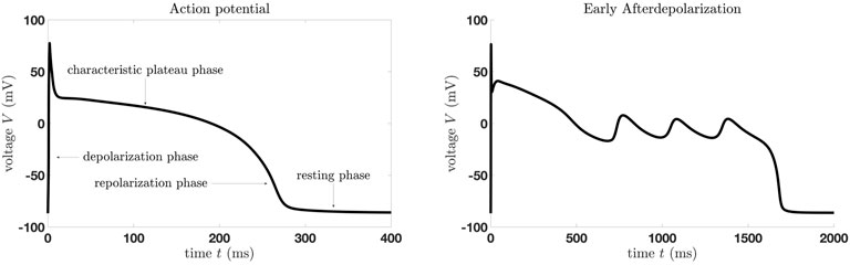
Figure 1. Simulations of a human ventricular cell model by Ten Tusscher and Panfilov from 2006 (TP06 model), [15]. (Left) Characteristic action potential. (Right) Early afterdepolarizations.

The presence of EADs strongly correlates with the onset of dangerous cardiac arrhythmia, including torsades de pointes, polymorphic ventricular tachycardia, and fibrillation, which are specific types of abnormal heart rhythms that can lead to sudden cardiac death [16, 17]. This potential spreading of EADs from cells to the whole heart, resulting in dangerous cardiac arrhythmias, provided the number of affected cells is large enough, is called EAD synchronization [16]. It is therefore highly important to fully understand the mechanism of such a phenomenon on the cellular as well as the tissue/organ level.

The main emphasis in this research field has been the modeling of cardiac muscle cells and the heart and the computational studies of these models [18, 19]. However, nowadays the focus moves towards systematic and more mathematical investigations of phenomena on the cellular level, such as EADs [20–23]. Bifurcation theory has proven to be a good tool for analyzing these systems by investigating changes in the qualitative or topological structure of a particular family of dynamic systems. It seeks to explain how the behavior of a system (e.g., its stable states or periodic cycles) changes with variation in a system parameter. In the context of cardiac dynamics, this often means studying how cardiac muscle cell dynamics such as action potentials or the heart rhythm can change—from normal sinus rhythm to arrhythmias such as tachycardia or fibrillation—when physiological parameters (such as ionic conductance, and pacing rate) are altered. Bifurcation theory is useful because it helps identify thresholds or critical points where the dynamics of the cardiac cell or the heart shift from one behavior to another, such as a small change in a physiological parameter leading to sudden cardiac arrhythmia. Bifurcation theory is particularly suited to systems with nonlinear dynamics, where other approaches fail; thus, bifurcation analysis is utilized in this manuscript.

This approach has mainly been used for studies of low- (up to four) dimensional ODE models [21, 24, 25]. Potential reasons for this are that bifurcation analysis of high-dimensional nonlinear systems is more challenging and might fail more easily due to imprecise settings. Further reasons are issues occurring due to the modeling of cell models themselves since they might not be smooth and regular enough. However, one main issue considering such a reduced problem is the loss of information [26, 27]. On the other hand, one can argue (for example, in [24, 25, 28]) that some sort of time-scale separation argument [29] is used to identify the gating variable of the $K^{+}$ current as the slowest variable to reduce the dimension $n$ of the system to $n-1$, $n\ge 3$ by using this gating variable as a bifurcation parameter. The advantage of this approach is that the analysis of the rapid subsystem is easier, but again, one may lose information cf. [27]. Moreover, this approach is not applicable to studying the effect of the ${\text{Ca}}^{2+}$ current or the ${\text{Na}}^{+}$ current since their gating variables are faster than that of the $K^{+}$ current.

The aim of the paper is to provide a mathematically feasible and physiologically realistic model for analyzing the electrophysiological dynamics of a cardiac muscle cell. Based on the reduced model, the bifurcation analysis enables the systematic investigation of the ionic current interactions, particularly the interaction of the calcium current with the slow and fast potassium currents. This analysis provides a deeper insight into how an enhanced calcium current in combination with reduced slow and fast potassium currents leads to EADs. In addition, the result of the bifurcation analysis allows quantification of these dangerous interactions. This study is divided into three parts. 1) To decode the dynamical structure that leads to EADs, we perform model reductions for the highly nonlinear and high-dimensional cell model. The reduced models are compared, and their advantages are emphasized. Furthermore, we show that the simplified models reproduce the dynamics of the full model. The aim is to obtain a model that is as simple and numerically efficient as possible to simulate and analyze it without losing information about the behavior of the voltage of the original model. These reduced models retain the essential nonlinear features of the full system but are better suited for mathematical analysis, such as bifurcation theory. 2) We investigate the reduced model by means of numerical bifurcation analysis and determine the complex behavior of the cardiac cell model. Furthermore, we will show that the occurrence of EADs in both the full and reduced model is determined by the same underlying bifurcation mechanism—a period doubling cascade. This shows that EADs arise on a generic route to chaos, which can also be captured and explained in simplified models. In the case of a stable period doubling cascade, chaos can also be simulated. Using bifurcation analysis, we identify critical transitions in the behavior of the system when key parameters are varied. In particular, we focus on the occurrence of EADs through a period doubling cascade. This approach allows (i) confirmation of the validity of the reduction; (ii) accurate determination of the conditions for the occurrence of EADs; (iii) predictions that can serve as a basis for further numerical or experimental studies. 3) Finally, based on these results, we will perform numerical simulations for the two-dimensional monodomain model to determine macroscale synchronization effects.

The motivation for this is as follows. Cardiac myocytes can exhibit complex oscillatory patterns, such as spiking and bursting, that are related to ion–current interactions. In addition to normal APs of a cardiac myocyte, certain types of cardiac arrhythmias can occur. These include certain types of cardiac arrhythmias that can lead to sudden cardiac death. Furthermore, irregular behavior such as (deterministic) chaos or chaotic EADs has been observed in both experimental and computational studies (cf. [30–33] and the references contained therein). Moreover, heart dynamics or the heart rhythm can react very sensitively to the influence of certain medications, and computational studies can provide new insights and help make better predictions cf. [34–39]. To this end, we modified and simplified the cardiac muscle cell model of Ten Tusscher and Panfilov from 2006 [15, 40] to perform numerical bifurcation analysis. This allows the investigation of the dynamics of the TP06 model and prediction of the occurrence of normal APs or cardiac arrhythmias, such as EADs. The focus of this study is on the model reduction and enhancement of the efficiency of the numerical bifurcation analysis without loss of information to the original TP06 model.

2 Methods

This section focuses on the methodology used in this manuscript, including the modeling of cardiac single models and the heart, as well as model reduction. Moreover, the bifurcation analysis and the numerical methods are discussed.

2.1 Cardiac single-cell modeling

Here, we briefly describe the cardiac model we will investigate in this paper. The mathematical modeling of action potentials (APs) of excitable biological cells, such as cardiac myocytes, has its origin in the Hodgkin–Huxley model [41]. Here, an approach was developed to model the APs of excitable biological cells through a system of ordinary differential equations (ODEs). These conductance-based models represent a minimal biophysical interpretation of excitable biological cells in which current flow across the membrane is due to the charging of membrane capacitance and movement of ions through ion channels that are selective for certain ion species. An initial stimulus activates the ion channels once a certain threshold potential is reached. Then, these ion channels open and/or close, allowing an ion current to flow that changes the membrane potential. This electrophysiological behavior of a cardiac myocyte is represented by the following ODE:

$C_m\frac{\mathrm{d}V}{\mathrm{d}t}=-{\mathrm{I}}_{\text{ion}}+{\mathrm{I}}_{\text{stim}},$

where $V$ denotes the voltage (in $mV$) and $t$ the time (in $ms$), while ${\mathrm{I}}_{\text{ion}}$ is the sum of all transmembrane ionic currents. The (epi-, mid-myo,- and endocardial) human ventricular TP06 model contains several different ion currents, ion pump, ion exchanger, and background currents:

${\mathrm{I}}_{\text{ion}}={\mathrm{I}}_{\text{K}1}+{\mathrm{I}}_{\text{to}}+{\mathrm{I}}_{\text{Kr}}+{\mathrm{I}}_{\text{Ks}}+{\mathrm{I}}_{\text{CaL}}+{\mathrm{I}}_{\text{NaK}}+{\mathrm{I}}_{\text{Na}}+{\mathrm{I}}_{\text{bNa}}+{\mathrm{I}}_{\text{NaCa}}+{\mathrm{I}}_{\text{bCa}}+{\mathrm{I}}_{\text{pK}}+{\mathrm{I}}_{\text{pCa}}.$

These currents depend on individual ionic conductances ${\mathrm{G}}_{\text{current}}$ and Nernst potentials ${\mathrm{E}}_{\text{current}}$. Moreover, they may depend on gating variables which are important for the activation and inactivation of ion currents. The gating variables satisfy the differential equation

$\frac{\mathrm{d}g}{\mathrm{d}t}=a_g\left(1-g\right)-b_{g}g=a_g-\left(a_g+b_g\right)g=\frac{g_{\infty }-g}{{\tau }_g},(1)$

where $g$ represents the gating variables, while $g_{\infty }≔g_{\infty }(V)=a_g\cdot {(a_g+b_g)}^{-1}$ denotes the equilibrium of the gating variable $g$ and ${\tau }_g≔{\tau }_g(V)={(a_g+b_g)}^{-1}$ its time scale. Furthermore, the ionic concentrations of the TP06 model from [15, 40] read as:

$\begin{array}{ll}\hfill \frac{\mathrm{d}\bar{R}}{\mathrm{d}t}& =-k_2{\left[Ca\right]}_{ss}\bar{R}+k_4\left(1-\bar{R}\right),\hfill \\ \hfill \frac{\mathrm{d}{\left[Ca\right]}_i}{\mathrm{d}t}& ={\text{Ca}}_{\text{ibufc}}\left(\left({\mathrm{I}}_{\text{leak}}-{\mathrm{I}}_{\text{up}}\right)\frac{V_{sr}}{V_c}+{\mathrm{I}}_{\text{xfer}}-\frac{\left({\mathrm{I}}_{\text{bCa}}+{\mathrm{I}}_{\text{pCa}}-2{\mathrm{I}}_{\text{NaCa}}\right)}{2V_{c}F}\right),\hfill \\ \hfill \frac{\mathrm{d}{\left[Ca\right]}_{sr}}{\mathrm{d}t}& ={\text{Ca}}_{\text{srbufsr}}\left({\mathrm{I}}_{\text{up}}-\left({\mathrm{I}}_{\text{rel}}+{\mathrm{I}}_{\text{leak}}\right)\right),\hfill \\ \hfill \frac{\mathrm{d}{\left[Ca\right]}_{ss}}{\mathrm{d}t}& ={\text{Ca}}_{\text{ssbufss}}\left(-\frac{{\mathrm{I}}_{\text{CaL}}}{2V_{ss}F}+{\mathrm{I}}_{\text{rel}}\frac{V_{sr}}{V_{ss}}-{\mathrm{I}}_{\text{xfer}}\frac{V_c}{V_{ss}}\right),\hfill \\ \hfill \frac{\mathrm{d}{\left[Na\right]}_i}{\mathrm{d}t}& =-\frac{{\mathrm{I}}_{\text{Na}}+{\mathrm{I}}_{\text{bNa}}+3{\mathrm{I}}_{\text{NaK}}+3{\mathrm{I}}_{\text{NaCa}}}{V_{c}F},\hfill \\ \hfill \frac{\mathrm{d}{[K]}_i}{\mathrm{d}t}& =-\frac{{\mathrm{I}}_{\text{K}1}+{\mathrm{I}}_{\text{to}}+{\mathrm{I}}_{\text{Kr}}+{\mathrm{I}}_{\text{Ks}}-2{\mathrm{I}}_{\text{NaK}}+{\mathrm{I}}_{\text{pK}}+{\mathrm{I}}_{\text{stim}}}{V_{c}F}.\hfill \end{array}$

Note that we do not specify the constants, but they are available in [15, 40] or in the code provided in [42]. Furthermore, the main ion currents except the sodium current are listed in the following.

$•$ L-type calcium current with gating variables $d$, $f$, $f2$ and $f_{\text{Cass}}$:

${\mathrm{I}}_{\text{CaL}}={\mathrm{G}}_{\text{CaL}}df{f}_2{f}_{\text{Cass}}\frac{4\left(V-15\right)F^2}{RT}\frac{0.25{\text{Ca}}_{\text{ss}}\exp \left.\left(2\left(V-15\right)\frac{F}{RT}\right)-{\text{Ca}}_{\text{o}}\right)}{\exp \left(2\left(V-15\right)\frac{F}{RT}\right)-1},$

$•$ transient outward current with gating variables $r$ and $s$:

${\mathrm{I}}_{\text{to}}={\mathrm{G}}_{\text{to}}rs\left(V-{\mathrm{E}}_{\text{K}}\right),$

$•$ slow delayed rectifier current with gating variable $x_s$:

${\mathrm{I}}_{\text{Ks}}={\mathrm{G}}_{\text{Ks}}{x}_s^2\left(V-{\mathrm{E}}_{\text{Ks}}\right),$

$•$ rapid delayed rectifier current with gating variables $x_{r_1}$ and $x_{r_2}$:

${\mathrm{I}}_{\text{Kr}}={\mathrm{G}}_{\text{Kr}}{x}_{r_1}{x}_{r_2}\left(V-{\mathrm{E}}_{\text{K}}\right),$

$•$ inward rectifier current:

${\mathrm{I}}_{\text{K}1}={\mathrm{G}}_{\text{K}1}{x}_{K{1}_{\infty }}\left(V-{\mathrm{E}}_{\text{K}}\right),$

where the gating variables satisfy the differential Equation 1. Finally, note the difference between the epi-, mid-myo-, and endocardial human ventricular TP06 model. There are two parts of the model which differ for these three cell types.

1. The modeling of the gating variable $s$ of the transient outward current ${\mathrm{I}}_{\text{to}}$ is different:

$s_{\infty }=\left\{\begin{array}{c}\frac{1}{1+e^{\frac{V+20}{5}}}\text{for\hspace{0.17em}epicardial\hspace{0.17em}and\hspace{0.17em}M\hspace{0.17em}cells},\hfill \\ \frac{1}{1+e^{\frac{V+28}{5}}}\text{for\hspace{0.17em}endocardial\hspace{0.17em}cells}\hfill \end{array}\right.$

and

${\tau }_s=\left\{\begin{array}{c}85e^{-\frac{{\left(V+45\right)}^2}{320}}+\frac{5}{1+e^{\frac{V-20}{5}}}+3\text{for\hspace{0.17em}epicardial\hspace{0.17em}and\hspace{0.17em}M\hspace{0.17em}cells},\hfill \\ 1000e^{-\frac{{\left(V+67\right)}^2}{1000}}+8\text{for\hspace{0.17em}endocardial\hspace{0.17em}cells}.\hfill \end{array}\right.$

2. The values of ${\mathrm{G}}_{\text{to}}$ and ${\mathrm{G}}_{\text{Ks}}$ differ:

${\mathrm{G}}_{\text{to}}=\left\{\begin{array}{c}0.294\frac{nS}{pF}\text{for\hspace{0.17em}epicardial\hspace{0.17em}and\hspace{0.17em}M\hspace{0.17em}cells},\hfill \\ 0.073\frac{nS}{pF}\text{for\hspace{0.17em}endocardial\hspace{0.17em}cells}\hfill \end{array}\right.$

and

${\mathrm{G}}_{\text{Ks}}=\left\{\begin{array}{c}0.392\frac{nS}{pF}\text{for\hspace{0.17em}epi}-\text{\hspace{0.17em}and\hspace{0.17em}endocardial\hspace{0.17em}cells},\hfill \\ 0.098\frac{nS}{pF}\text{for\hspace{0.17em}M\hspace{0.17em}cells}.\hfill \end{array}\right.$

For a full description of the variables involved, please see [15, 40].

This also implies that we only need one proper bifurcation analysis with respect to ${\mathrm{G}}_{\text{Ks}}$ for epicardial and M cells since the models are different only in ${\mathrm{G}}_{\text{Ks}}$. Furthermore, we need a separate analysis for endocardial cells. This also explains why the trajectories in Figures 2, 3 are different. For the simulations in Figures 2, 3, we used the same setting as in [15], except for the value ${\mathrm{G}}_{\text{Kr}}$, which we set to $18\%$ of the original value and the value ${\mathrm{G}}_{\text{GaL}}$, which we have chosen as five times bigger than that in [15]. Therefore, the M cell enters a region where EADs occur.

Figure 2

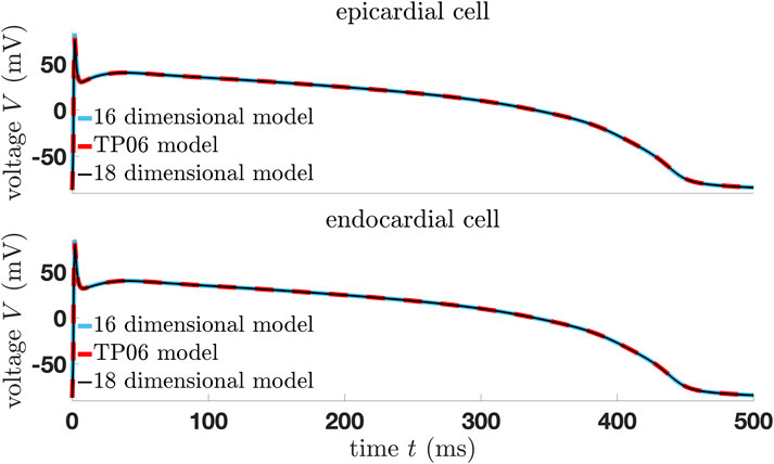
Figure 2. Comparison of the modified models and original TP06 human ventricular epi- and endocardial cell model.

Figure 3

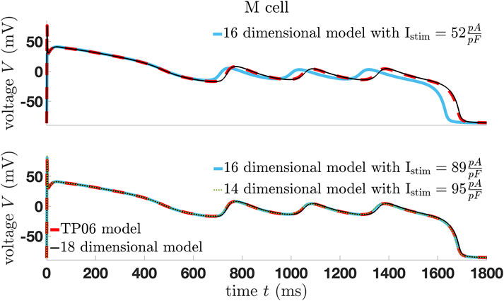
Figure 3. Comparison of the modified and original TP06 human ventricular mid-myocardial cell model.

2.2 Monodomain model

To model the heart, different types of reaction–diffusion type systems are available, where the focus is on different research questions, and their complexities vary (cf. e.g., [43–48]). This paper focuses on the two-dimensional monodomain model since it is used to model the original TP06 model (cf. [15, 40]). In addition to this, monodomain models have been shown to be a good approximation for wave propagation in cardiac tissue (e.g., [49]) and are well studied (e.g., [50, 51]). The monodomain model reads as follows:

$\frac{\lambda }{1+\lambda }\nabla \cdot \left(M_i\nabla V\right)=\chi \left(C_m\frac{\partial V}{\partial t}+{\mathrm{I}}_{\text{ion}}\left(V,g\right)-{\mathrm{I}}_{\text{stim}}\right)(2)$

with equal anisotropy rates $M_e=\lambda M_i$, where $\lambda$ is a scalar constant, $\nabla$ is the spatial gradient, $M_i$ and $M_e$ denotes the intra- and extracellular conductivity tensors, and $\chi$ is the membrane surface area per unit volume. Moreover, the system is equipped with Neumann boundary conditions, $(M_i\nabla V)\cdot \vec{n}=0$, where $\vec{n}$ denotes the normal vector. In the fashion of [39], we write the monodomain Equation 2 as a reaction–diffusion system, which it is:

$\frac{\partial V}{\partial t}=D\mathrm{\Delta }V-\frac{{\mathrm{I}}_{\text{ion}}\left(V,g\right)+{\mathrm{I}}_{\text{stim}}}{C_m},(3)$

where $D$ denotes the diffusion coefficient $D=\frac{\lambda }{1+\lambda }\frac{M_i}{\chi }\frac{1}{C_m}$. Moreover, we use the same mesh, time, and space discretization and stimulus, as in [39] (Table 1).

Table 1

Table 1. Mesh, stimulation, and diffusion parameters.

Notice that for normal AP simulations, a time step of $\mathrm{\Delta }t=0.05ms$ is used, while for the simulations of EAD settings, it is $\mathrm{\Delta }t=0.02ms$.

2.3 Model reduction

The aim of model reduction is to simplify a complex mathematical model while retaining its essential behaviors and properties so that the reduced model can be calculated more quickly and analyzed more easily. Therefore, we modify and simplify the TP06 cell model and then compare the dynamics of the resulting three modified TP06 models—one 18-dimensional, one 16-dimensional, and one 14-dimensional system of ordinary differential equations (ODEs). The 18-dimensional model is in the fashion of [52, 53] and perfectly represents the original model, while the 16-dimensional model gives a perfect approximation of the original model in case we modify the initial stimulus. The same applies to the 14-dimensional model. Notice that without the modification of the initial stimulus, the models show very similar dynamics compared to the original one; however, the trajectories do not perfectly coincide with that from the TP06 model.

2.4 Bifurcation theory

Very powerful tools to systematically analyze the dynamics of cardiac myocytes are bifurcation theory [54] and geometric singular perturbation theory [55] (see for instance, recent studies in [21, 26, 56–65] and the references contained therein). These computational studies can be used to develop new therapies and help in improving clinical decisions [66–70].

In general, the state of a physical system can be observed when it is stable, and one expects that a small change in a system parameter should not change its dynamics. Rather, stable solutions can be expected to continuously change in unique ways. No dramatic change is observed when varying any parameter, as long as a continuous solution branch retains its stability. However, when a certain physical parameter exceeds a threshold, the physical system may be forced to change its dynamics, and complex behavior may result. Therefore, bifurcation theory is used to explain certain phenomena and dynamics of the TP06 model of Ten Tusscher and Panfilov from 2006 (cf. [15]).

One requirement to be able to apply bifurcation theory is that the investigated system is sufficiently smooth. However, this is not the case for the original TP06 model (reported, for instance, in [53, 71]). In [53], the authors modified the sodium current ${\mathrm{I}}_{\text{Na}}$ similar to the approach used in [52], while in [71] the sodium current ${\mathrm{I}}_{\text{Na}}$ was modified based on [72]. Both approaches enable (numerical) bifurcation analysis with slight differences. The advantage of the approach used in [53] is that the remodeled system almost always perfectly fits the original TP06 model without changing the stimulus, while the ansatz in [71] leads to an almost perfect remodeling of the original TP06 model. On the other hand, the ansatz in [71] results in a lower-dimensional model, and therefore the bifurcation analysis is more efficient. These advantages and disadvantages must be considered.

The important bifurcations in this study are 1) Andronov–Hopf bifurcations; 2) torus bifurcations; 3) period-doubling bifurcations [54]. An Andronov–Hopf bifurcation occurs when a fixed point of a dynamic system changes its stability and a limit cycle (periodic orbit) occurs. In a supercritical Andronov–Hopf bifurcation, a stable limit cycle occurs. In the subcritical case, an unstable limit cycle appears. The Lyapunov coefficient determines the nature of the Andronov–Hopf bifurcation. Its sign indicates whether the bifurcation is supercritical (negative coefficient, stable limit cycle) or subcritical (positive coefficient, unstable limit cycle). It quantifies the nonlinear effects near the bifurcation point. A torus bifurcation (or Neimark–Sacker bifurcation) occurs when a limit cycle loses stability and a quasiperiodic orbit emerges on a torus. The system’s dynamics then evolve with two incommensurate frequencies, leading to motion on a 2D torus instead of a simple periodic loop. At period-doubling bifurcations, the periodic behavior of the system changes, giving rise to a new orbit with twice the period. Moreover, a period-doubling cascade is clearly linked to the occurrence of EADs and, in the case of a supercritical period-doubling cascade, is clearly linked to chaos (e.g., [30]).

2.5 Numerical methods

For our simulations, we utilized MATLAB R2023b and Python 3.9 with FEniCS [73, 74]. To solve the ODE system, we mainly use the MATLAB ode solver ode15s with a relative tolerance of $10^{-13}$ and an absolute tolerance of $10^{-18}$. For the monodomain model, the two-dimensional simulations are done in FEniCS, where the coupled ODE–PDE system is solved using cbcbeat [75] or fenics-beat [76], which are Python/FEniCS-based libraries for running cardiac electrophysiology simulations. Note that cbcbeat and fenics-beat use a second-order splitting scheme with the Crank–Nicolson method for time stepping. Moreover, the Rush and Larsen scheme [77] is used to integrate the gating variables in time. For the bifurcation analysis, we used CL_MATCONT, a continuation toolbox for MATLAB [78, 79]. Codes are available via [42].

3 Results

The modifications we present here reduce the complexity of the 19-dimensional TP06 model in several steps to an 18-, 16-, and 14-dimensional system with astonishing consistency with the original model (Figures 2, 3). Here, we changed the conductance of the slow delayed rectifier current ${\mathrm{I}}_{\mathrm{K}\mathrm{s}}$, rapid delayed rectifier current ${\mathrm{I}}_{\mathrm{K}\mathrm{r}}$, and the L-type calcium current ${\mathrm{I}}_{\mathrm{C}\mathrm{a}\mathrm{L}}$ such that $({\mathrm{G}}_{\mathrm{K}\mathrm{s}},{\mathrm{G}}_{\mathrm{K}\mathrm{r}},{\mathrm{G}}_{\mathrm{C}\mathrm{a}\mathrm{L}})\to ({\mathrm{G}}_{\mathrm{K}\mathrm{s}},0.18\cdot {\mathrm{G}}_{\mathrm{K}\mathrm{r}},5\cdot {\mathrm{G}}_{\mathrm{C}\mathrm{a}\mathrm{L}})$.

As well as the modifications and model reduction which we will present in the next section, we have to adjust the initial stimulus for the 16-dimensional model in Figure 2, using ${\mathrm{I}}_{\text{stim}}=89\frac{pA}{pF}$ instead of ${\mathrm{I}}_{\text{stim}}=52\frac{pA}{pF}$. Moreover, the effect of the different stimuli can be clearly observed in Figure 3. In the first row of Figure 3, an initial stimulus of ${\mathrm{I}}_{\text{stim}}=52\frac{pA}{pF}$ is applied to the 16-dimensional model. Although the trajectories do not match perfectly, the dynamics are similar. In the second row of Figure 3, perfectly matching trajectories of the TP06 model and its different versions are shown, highlighting whether a different stimulus is applied. Notice that the MATLAB code to produce Figures 2, 3 is provided in [42]. Using this code, the readers can also convince themselves that the modified systems effectively approximate the original system.

As well as the model reduction, the focus is on the complex dynamics these models can develop. Numerical bifurcation analysis is applied, highlighting that a reduction in the slow and rapid delayed rectifier current, ${\mathrm{I}}_{\mathrm{K}\mathrm{s}}$ and ${\mathrm{I}}_{\mathrm{K}\mathrm{r}}$, in combination with an enhanced L-type calcium current ${\mathrm{I}}_{\mathrm{C}\mathrm{a}\mathrm{L}}$, force the system to develop EADs. This can be linked to the existence of a subcritical period-doubling cascade. Moreover, it is shown that no chaos may appear.

Finally, we investigate the 2D synchronization effects. In the 2D case, we highlight that the monodomain equation’s dependence on the system parameters develops stable spiral waves, but wave break-up may also appear (cf. Figure 10) due to the EAD developed by the cellular model.

3.1 Model modification and reduction

First, we remove the ODE representing the intracellular ion concentration ${[K]}_i$ and set ${[K]}_i$ constant equal to the initial concentration ${[K]}_i$ of the TP06 model, ${[K]}_i=138.3mM$. In [80], it was postulated that models for cardiac cells that account for changes in intracellular ion concentrations violate a conservation principle. Moreover, it turned out that the variation in the concentration ${[K]}_i$ is rather small (cf. [71]). Consequently, these systems never reach a steady state—a resting potential—which is required to be able to apply bifurcation theory. All modifications we present below are tabularly collected and compared in the first section of the supplementary material.

3.1.1 18 dimensional model

As indicated in [71], the first issue is in the modeling of the sodium current in (40, 15)

${\mathrm{I}}_{\text{Na}}={\mathrm{G}}_{\text{Na}}{m}^{3}hj\left(V-{\mathrm{E}}_{\text{Na}}\right),$

where ${\mathrm{G}}_{\text{Na}}$ denotes the ionic conductance and ${\mathrm{E}}_{\text{Na}}$ the Nernst potential, while the different gating variables $m$, $h$, and $j$ satisfy differential Equation 1. To be more precise, the issue appears in the modeling of the gating variables $h$ and $j$ since the voltage-dependent functions ${\alpha }_h$, $,{\beta }_h$, ${\alpha }_j$, and $,{\beta }_j$ are not continuous:

$\begin{array}{ll}\hfill {\alpha }_h& =\left\{\begin{array}{cc}0\hfill & \text{\hspace{0.17em}if\hspace{0.17em}}V\ge -40mV,\hfill \\ 0.057\exp \left(\frac{-\left(V+80\right)}{6.8}\right)\hfill & \text{\hspace{0.17em}if\hspace{0.17em}}V<-40mV,\hfill \end{array}\right.\hfill \\ \hfill b_h& =\left\{\begin{array}{cc}\frac{0.77}{0.13\left(1+\exp \left(\frac{-\left(V+10.66\right)}{11.1}\right)\right)}\hfill & \text{\hspace{0.17em}if\hspace{0.17em}}V\ge -40mV,\hfill \\ \left(2.7e^{0.079V}+3.1\cdot 10^5{e}^{0.3485V}\right)\hfill & \text{\hspace{0.17em}if\hspace{0.17em}}V<-40mV,\hfill \end{array}\right.\hfill \\ \hfill {\alpha }_j& =\left\{\begin{array}{cc}0\hfill & \text{\hspace{0.17em}if\hspace{0.17em}}V\ge -40mV,\hfill \\ \left(-2.5428\cdot 10^4{e}^{0.2444V}-6.948\cdot 10^{-6}{e}^{-0.04391V}\right)\frac{V+37.78}{1+e^{0.311\left(V+79.23\right)}}\hfill & \text{\hspace{0.17em}if\hspace{0.17em}}V<-40mV,\hfill \end{array}\right.\hfill \\ \hfill b_j& =\left\{\begin{array}{cc}0.6\frac{e^{0.057V}}{1+e^{-0.1\left(V+32\right)}}\hfill & \text{\hspace{0.17em}if\hspace{0.17em}}V\ge -40mV,\hfill \\ \frac{0.02424e^{-0.01052V}}{1+e^{-0.1378\left(V+40.14\right)}}\hfill & \text{\hspace{0.17em}if\hspace{0.17em}}V<-40mV,\hfill \end{array}\right.\hfill \end{array}$

(cf. [40]). In the fashion of [52, 53], we introduce a new function

$u=\frac{1}{1+e^{-5\left(V+40\right)}},$

(cf. Supplementary Figure S8) and remodel the rate constants ${\alpha }_h,{\beta }_h,{\alpha }_j$ and ${\beta }_j$ as follows:

$\begin{array}{ll}\hfill {\alpha }_h& =\left(1-u\right)0.057e^{\frac{-\left(V+80\right)}{6.8}},\hfill \\ \hfill {\beta }_h& =\frac{0.77}{0.13\left(1+e^{\frac{-\left(V+10.66\right)}{11.1}}\right)}u+\left(1-u\right)\left(2.7e^{0.079V}+3.1\cdot 10^5{e}^{0.3485V}\right),\hfill \\ \hfill {\alpha }_j& =\left(1-u\right)\left(-2.5428\cdot 10^4{e}^{0.2444V}-6.948\cdot 10^{-6}{e}^{-0.04391V}\right)\frac{V+37.78}{1+e^{0.311\left(V+79.23\right)}},\hfill \\ \hfill {\beta }_j& =0.6\frac{e^{0.057V}}{1+e^{-0.1\left(V+32\right)}}u+\left(1-u\right)\frac{0.02424e^{-0.01052V}}{1+e^{-0.1378\left(V+40.14\right)}}.\hfill \end{array}$

Now, the modified model is sufficiently smooth without any discontinuity. Therefore, bifurcation analysis is applicable, and no further modifications are needed to fit the original model. Note that the function $u$ is modeled in such a way that $u=1$ for $V=-40mV$ to represent the switching modeled in [40] of ${\alpha }_h,{\beta }_h,{\alpha }_j$ and ${\beta }_j$ at $V=-40mV$, while the factor “$-5$” might be improvable (cf. Supplementary Figure S8–10).

3.1.2 16 dimensional model

A further way to avoid the issue with the discontinuity of the rate constants ${\alpha }_h,{\beta }_h,{\alpha }_j$ and ${\beta }_j$ is to notice that the equilibrium of $h$ and $j$ is equal. In [71], the gating variables $h$ and $j$ are reformulated to one new gating variable $v$, the sodium current is modified to

${\mathrm{I}}_{\text{Na}}={\mathrm{G}}_{\text{Na}}{m}^3{v}^2\left(V-{\mathrm{E}}_{\text{Na}}\right),$

and a new time scale is introduced such that $v$ satisfies (Equation 2) with

$v_{\infty }=h_{\infty }=j_{\infty }=\frac{1}{{\left(1+e^{\frac{V+71.55}{7.43}}\right)}^2}$

The time relaxation constant is given by

${\tau }_v=0.25+\frac{2.24\cdot v_{\infty }}{\left(1-\tanh \left(6.468+0.07V\right)\right)},$

which could probably be improved. However, we realized that instead of considering a 17-dimensional model, it is more practical to set $v=v_{\infty }=h_{\infty }=j_{\infty }$ and to adjust the initial stimulus. This removes the discontinuity, and in addition, we reduce the model by a further dimension.

3.1.3 14 dimensional model

Finally, in this fashion and motivated by [81], we also fixed two further gating variables equal to their steady-state solutions—that is, we fixed the gating variable $r$ of the transient outward current ${\mathrm{I}}_{\text{to}}$ and the gating variable $x_{r_2}$ of the rapid delayed rectifier current ${\mathrm{I}}_{\text{Kr}}$ such that

$r=r_{\infty }=\frac{1}{1+e^{\frac{-\left(V+20\right)}{6}}}\text{and}{x}_{r_2}=x_{{r_2}_{\infty }}=\frac{1}{1+e^{\frac{V+88}{24}}}.$

This again requires modification of the initial stimulus, which must be higher than the 16-dimensional model. However, this simplified model shows a remarkably accurate approximation of the original model, and additionally, it is much less challenging to analyze, which we will highlight later in more detail.

3.2 Bifurcation analysis of the cardiac single-cell model

The aim of the study is to make statements about the behavior of the trajectories and the dynamics of the TP06 system. To this end, it investigates the stability and bifurcations of the modified systems (cf. [30, 53, 54, 82]). Moreover, we provide the corresponding codes in [42].

A bifurcation of a dynamic system is a qualitative change in its dynamics caused by the change of parameters. Therefore, we study the modified TP06 model by means of (numerical) bifurcation analysis using CL_MATCONT, a continuation toolbox for MATLAB [78, 79]. We consider an autonomous system of ordinary differential equations, where the right-hand side of this system depends on several state variables and parameters. Therefore, we consider the modified TP06 models, containing 18, 16, or 14 state variables, without initial stimulus for the bifurcation analysis, and we will focus our study on the effect of a deficit in the fast and slow potassium currents ${\mathrm{I}}_{\text{Kr}}$ and ${\mathrm{I}}_{\text{Ks}}$, respectively, and an enhancement in the L-type calcium current ${\mathrm{I}}_{\mathrm{C}\mathrm{a}\mathrm{L}}$.

The starting point of the bifurcation analysis is to determine an equilibrium of the modified autonomous system. To this end, the algebraic equations are solved thus:

$\begin{array}{ll}\hfill 0& ={\mathrm{I}}_{\text{K}1}+{\mathrm{I}}_{\text{to}}+{\mathrm{I}}_{\text{Kr}}+{\mathrm{I}}_{\text{Ks}}+{\mathrm{I}}_{\text{CaL}}+{\mathrm{I}}_{\text{NaK}}+{\mathrm{I}}_{\text{Na}}+{\mathrm{I}}_{\text{bNa}}+{\mathrm{I}}_{\text{NaCa}}+{\mathrm{I}}_{\text{bCa}}+{\mathrm{I}}_{\text{pK}}+{\mathrm{I}}_{\text{pCa}},\hfill \\ \hfill 0& =-k_2{\left[Ca\right]}_{ss}\bar{R}+k_4\left(1-\bar{R}\right),\hfill \\ \hfill 0& ={\text{Ca}}_{\text{ibufc}}\left(\left({\mathrm{I}}_{\text{leak}}-{\mathrm{I}}_{\text{up}}\right)\frac{V_{sr}}{V_c}+{\mathrm{I}}_{\text{xfer}}-\frac{\left({\mathrm{I}}_{\text{bCa}}+{\mathrm{I}}_{\text{pCa}}-2{\mathrm{I}}_{\text{NaCa}}\right)}{2V_{c}F}\right),\hfill \\ \hfill 0& ={\text{Ca}}_{\text{srbufsr}}\left({\mathrm{I}}_{\text{up}}-\left({\mathrm{I}}_{\text{rel}}+{\mathrm{I}}_{\text{leak}}\right)\right),\hfill \\ \hfill 0& ={\text{Ca}}_{\text{ssbufss}}\left(-\frac{{\mathrm{I}}_{\text{CaL}}}{2V_{ss}F}+{\mathrm{I}}_{\text{rel}}\frac{V_{sr}}{V_{ss}}-{\mathrm{I}}_{\text{xfer}}\frac{V_c}{V_{ss}}\right),\hfill \\ \hfill 0& =-\frac{{\mathrm{I}}_{\text{Na}}+{\mathrm{I}}_{\text{bNa}}+3{\mathrm{I}}_{\text{NaK}}+3{\mathrm{I}}_{\text{NaCa}}}{V_{c}F}\hfill \end{array}$

with $g\equiv g_{\infty }(V)$, where $g$ represents the gating variables. The next step is to derive the stability of the equilibrium to determine the eigenvalues of the Jacobian or using the Routh–Hurwitz criterion [30, 82]. If we do so, we are able to determine the stability of the modified systems dependent on the ionic conductances ${\mathrm{G}}_{\text{Ks}}$, ${\mathrm{G}}_{\text{Kr}}$, and ${\mathrm{G}}_{\text{CaL}}$ (Figure 4). Here, we have stable (black surfaces) and unstable regions (gray surfaces).

Figure 4

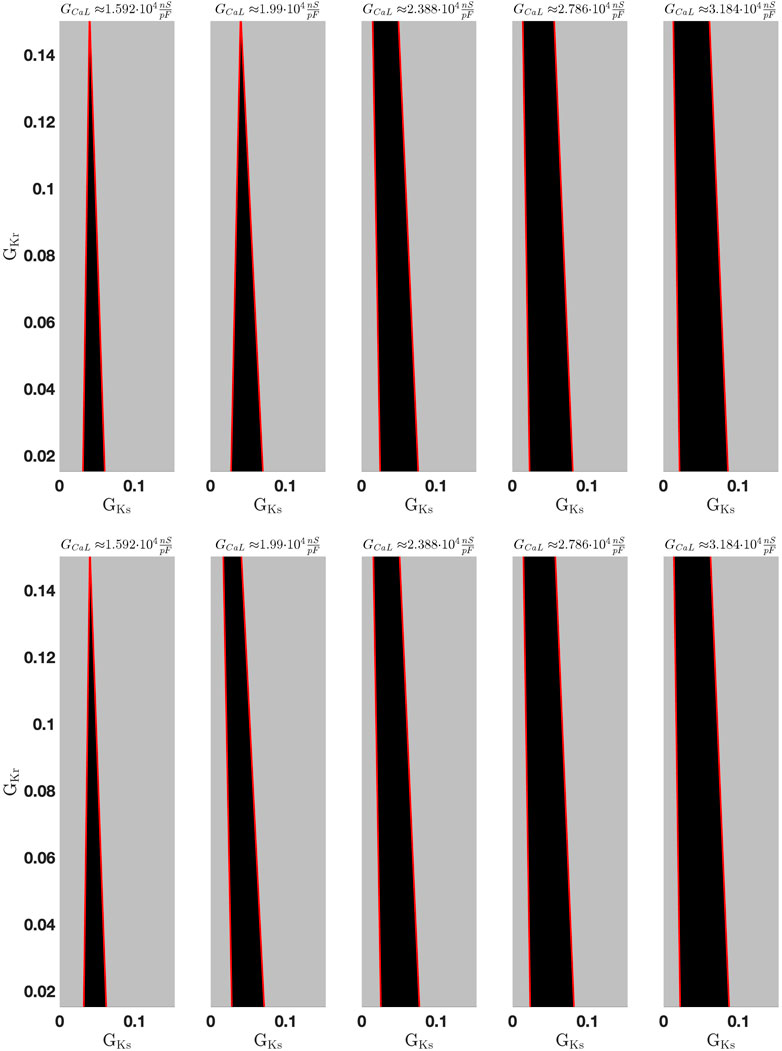
Figure 4. Multiple bifurcation analysis. Stable (black surface) and unstable (gray surface) regions projected on the $({\mathrm{G}}_{\mathrm{K}\mathrm{s}},{\mathrm{G}}_{\mathrm{K}\mathrm{r}},{\mathrm{G}}_{\mathrm{C}\mathrm{a}\mathrm{L}})$-space. (Upper) epicardial cell. (Lower) endocardial cell.

The unstable region allows the system to oscillate; after an initial stimulus the trajectory—the time-dependent voltage variation of the ODE model—can either develop normal APs or other oscillatory behavior such as EADs or some sort of ventricular tachycardia, which cannot be specified at this stage. However, in case the trajectory enters the stable region, it will reach a stable equilibrium—in this case not the resting potential, the potential becomes $V\approx 0mV$. This corresponds to sudden death, because if multiple cardiac cells lose their membrane potential, the heart can no longer generate electrical impulses, leading to asystole (cardiac arrest). Figure 4 also indicates that for increasing ${\mathrm{G}}_{\text{CaL}}$ and decreasing ${\mathrm{G}}_{\text{Ks}}$ and ${\mathrm{G}}_{\text{Kr}}$, the stable area becomes larger and the risk of sudden death increases, where the possibility that the voltage becomes continuously 0 is increased. This result is also compatible with the current state of knowledge. Moreover, Figure 4 also shows two red lines—the Andronov–Hopf bifurcation curves. At an Andronov-Hopf bifurcation, the system changes stability via a pair of purely imaginary eigenvalues—${\lambda }_{\mathrm{1,2}}=\pm \mathbf{i}{\omega }_0$ and ${\omega }_0>0$—and a limit cycle appears.

Note that the standard value ${\mathrm{G}}_{\text{Kr}}$ is $0.153\frac{nS}{pF}$. Therefore, in case ${\mathrm{G}}_{\text{CaL}}$ does not increase too much and ${\mathrm{G}}_{\text{Ks}}$ remains its standard value, the risk that the cardiac myocyte TP06 model develops sudden death is small to almost 0. However, if ${\mathrm{G}}_{\text{CaL}}$ increases, such as by a factor 5, and ${\mathrm{G}}_{\text{Kr}}$ is small, the risk of a sudden death increases and the M cells already develop EADs for the standard value of ${\mathrm{G}}_{\text{Ks}}$ (Figure 3). Again, this is reasonable and compatible with the current state of knowledge since it is known that EADs can be related to the limit cycle bifurcating from an Andronov–Hopf bifurcation (e.g., [30, 71, 82]), and from a medical point of view, EADs can be precursors to sudden cardiac death.

Our goal is to examine the parameter set $({\mathrm{G}}_{\mathrm{K}\mathrm{s}},{\mathrm{G}}_{\mathrm{K}\mathrm{r}},{\mathrm{G}}_{\mathrm{C}\mathrm{a}\mathrm{L}})$ and to better understand the behavior of the (endocardial) cell model and compare the stationary dynamics of the 18-, 16-, and 14-dimensional model. A more practical way of analyzing a dynamic system by means of bifurcation theory is to use the continuation algorithm from [78, 79]. Choosing the parameter set $({\mathrm{G}}_{\mathrm{K}\mathrm{s}},{\mathrm{G}}_{\mathrm{K}\mathrm{r}},{\mathrm{G}}_{\mathrm{C}\mathrm{a}\mathrm{L}})\to ({\mathrm{G}}_{\mathrm{K}\mathrm{s}},0.1\cdot {\mathrm{G}}_{\mathrm{K}\mathrm{r}},5\cdot {\mathrm{G}}_{\mathrm{C}\mathrm{a}\mathrm{L}})$ and ${\mathrm{G}}_{\mathrm{K}\mathrm{s}}$ as a bifurcation parameter, we obtain two supercritical Andronov–Hopf bifurcations (Tables 2, 3) which both generate a stable limit cycle, and thus the bifurcating limit cycles are both stable. Between these Andronov–Hopf bifurcations, the system exhibits the stable equilibrium branch. Tables 2, 3 show that the three different models have almost identical Andronov–Hopf bifurcations.

Table 2

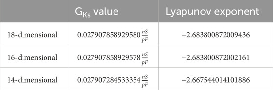
Table 2. Comparison: First supercritical Andronov–Hopf bifurcation.

Table 3

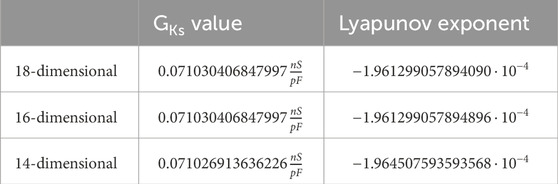
Table 3. Comparison: second supercritical Andronov–Hopf bifurcation.

We give all eigenvalues corresponding to the Andronov–Hopf bifurcations from Tables 2, 3 in Supplementary Tables S1, 2.

Starting a limit cycle continuation from the second supercritical Andronov–Hopf bifurcation, we derive a limit cycle branch containing a torus bifurcation and a (first) period-doubling bifurcation (cf. Table 4). Note that this limit cycle branch is the reason for the occurrence of both AP and EADs, which we will highlight later in more detail.

Table 4

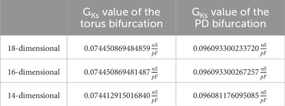
Table 4. Comparison: torus bifurcation and period-doubling (PD) bifurcation of the first limit cycle branch.

Again, we give all characteristic multipliers corresponding to the period-doubling bifurcations from Table 4 in Supplementary Table S3. It is remarkable that, for 18, 16, and 14 dimensions, not only are the equilibrium curves identical, which is obvious, but the stability and the bifurcation points are also identical to a certain degree, which is visible in Tables 2–4. This is also reflected in Figure 5, where no are apparent differences. The first limit cycle branch (red surface) of the three simplified models bifurcates from a supercritical Andronov–Hopf bifurcation (red dot). At this bifurcation, the equilibrium curve (black line: the dashed part represents the unstable branch, the solid part the stable branch) also changes stability.

Figure 5

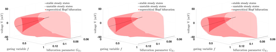
Figure 5. Comparison of the bifurcation diagrams using ${\mathrm{G}}_{\mathrm{K}\mathrm{s}}$ as a bifurcation parameter with value shifts ${\mathrm{G}}_{\mathrm{K}\mathrm{r}}\to 0.1\cdot {\mathrm{G}}_{\mathrm{K}\mathrm{r}}$ and ${\mathrm{G}}_{\mathrm{C}\mathrm{a}\mathrm{L}}\to 5\cdot {\mathrm{G}}_{\mathrm{C}\mathrm{a}\mathrm{L}}$. (Left) 18-dimensional. (middle) 16-dimensional, and (right) 14-dimensional models.

Note that fixing more gating variables equal to its steady-state solution will not change the equilibrium curve, but it will change its stability and potential bifurcations points and, therefore, the dynamics of the whole system. Furthermore, Figure 6 shows the limitation of the 18-dimensional model since for the M cells, the trajectory does not fit perfectly. Moreover, the stimuli for the 16- and 14-dimensional models differ from those in Figure 3. In any case, normal AP is well represented by the simplified models. In the case of more complex patterns such as EADs, the general dynamics of all models are identical, but finding the correct basin of attraction modifying the stimulus is more difficult.

Figure 6

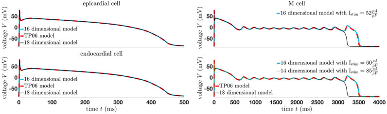
Figure 6. Comparison of the trajectories of the modified models using the standard value of ${\mathrm{G}}_{\mathrm{K}\mathrm{s}}$ with value shifts ${\mathrm{G}}_{\mathrm{K}\mathrm{r}}\to 0.1\cdot {\mathrm{G}}_{\mathrm{K}\mathrm{r}}$ and ${\mathrm{G}}_{\mathrm{C}\mathrm{a}\mathrm{L}}\to 5\cdot {\mathrm{G}}_{\mathrm{C}\mathrm{a}\mathrm{L}}$.

Our next aim is to study the 14-dimensional epicardial TP06 model in more detail by means of bifurcation analysis. Our focus is on a situation like in Figure 6, where we use ${\mathrm{G}}_{\mathrm{K}\mathrm{s}}$ as the bifurcation parameter and consider value shifts ${\mathrm{G}}_{\mathrm{K}\mathrm{r}}\to 0.1\cdot {\mathrm{G}}_{\mathrm{K}\mathrm{r}}$ and ${\mathrm{G}}_{\mathrm{C}\mathrm{a}\mathrm{L}}\to 5\cdot {\mathrm{G}}_{\mathrm{C}\mathrm{a}\mathrm{L}}$. We thus have a reduced rapid delayed rectifier current and an enhanced L-type calcium current. Utilizing the bifurcation analysis, we can extract the behavior and dynamics of the system. Starting a numerical continuation from a steady state solution, we find two supercritical Andronov–Hopf bifurcations (cf. Table 5).

Table 5

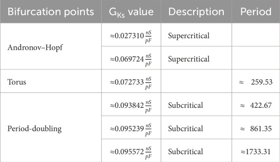
Table 5. Bifurcation for the 14-dimensional epicardial cell model with $({\mathrm{G}}_{\mathrm{K}\mathrm{s}},{\mathrm{G}}_{\mathrm{K}\mathrm{r}},{\mathrm{G}}_{\mathrm{C}\mathrm{a}\mathrm{L}})\to ({\mathrm{G}}_{\mathrm{K}\mathrm{s}},0.1\cdot {\mathrm{G}}_{\mathrm{K}\mathrm{r}},5\cdot {\mathrm{G}}_{\mathrm{C}\mathrm{a}\mathrm{L}})$.

From these bifurcation points, a stable limit cycle branch bifurcates each. Following the limit cycle branch from the second Andronov–Hopf bifurcation $({\mathrm{G}}_{\mathrm{K}\mathrm{s}}\approx 0.069724\frac{nS}{pF})$, we find a torus bifurcation and a first period-doubling bifurcation. Furthermore, the limit cycle branch changes stability; finally, it will collide with the equilibrium curve and terminate there (cf. Figure 7 and Supplementary Figure S7).

Figure 7

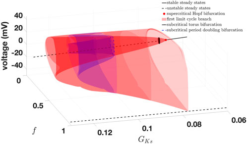
Figure 7. Bifurcation diagram of the 14-dimensional epicardial cell model with $({\mathrm{G}}_{\mathrm{K}\mathrm{s}},{\mathrm{G}}_{\mathrm{K}\mathrm{r}},{\mathrm{G}}_{\mathrm{C}\mathrm{a}\mathrm{L}})\to ({\mathrm{G}}_{\mathrm{K}\mathrm{s}},0.1\cdot {\mathrm{G}}_{\mathrm{K}\mathrm{r}},5\cdot {\mathrm{G}}_{\mathrm{C}\mathrm{a}\mathrm{L}})$, where ${\mathrm{G}}_{\mathrm{K}\mathrm{s}}$ is used as a bifurcation parameter. The bifurcation diagram contains the second Andronov–Hopf bifurcation, the first two limit-cycle branches, the torus bifurcation, and the first period-doubling bifurcation.

This behavior is similar for all investigated combinations of $({\mathrm{G}}_{\mathrm{K}\mathrm{s}},{\mathrm{G}}_{\mathrm{K}\mathrm{r}},{\mathrm{G}}_{\mathrm{C}\mathrm{a}\mathrm{L}})$. However, the position of the points varies (cf. Tables 5, 6). Starting a continuation from the first period-doubling bifurcation, we find a second limit cycle branch containing a second period-doubling bifurcation (cf. again Figure 7). Taking this approach further results in an unstable period-doubling cascade; in Figure 8, we zoom in on the region with the first four limit cycle branches.

Table 6

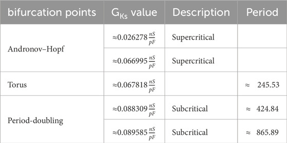
Table 6. Bifurcation for the 14-dimensional epicardial cell model with $({\mathrm{G}}_{\mathrm{K}\mathrm{s}},{\mathrm{G}}_{\mathrm{K}\mathrm{r}},{\mathrm{G}}_{\mathrm{C}\mathrm{a}\mathrm{L}})\to ({\mathrm{G}}_{\mathrm{K}\mathrm{s}},0.18\cdot {\mathrm{G}}_{\mathrm{K}\mathrm{r}},5\cdot {\mathrm{G}}_{\mathrm{C}\mathrm{a}\mathrm{L}})$.

Figure 8

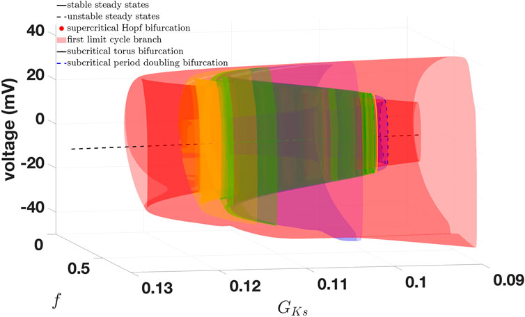
Figure 8. Zoom of Figure 7 containing the first four limit cycle branches.

To highlight the transition at each limit cycle bifurcation, Figure 9 shows four trajectories at the torus bifurcation and the first three period-doubling bifurcations (from left to right).

Figure 9

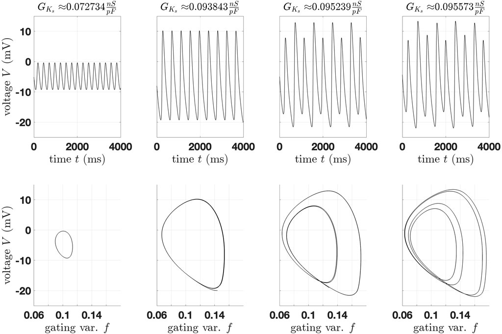
Figure 9. Comparison of trajectories of the 14-dimensional epicardial cell model (“action potentials” at the torus bifurcation and the first three period-doubling bifurcations (from left to right).

We start a simulation with an initial value on the limit cycle and with the corresponding ${\mathrm{G}}_{\mathrm{K}\mathrm{s}}$ value. Further details are in Supplementary Figures S1–S6.

Based on the bifurcation diagram, we can identify a ${\mathrm{G}}_{\mathrm{K}\mathrm{s}}$ region where EADs may appear. This region is clearly linked to the period-doubling cascade; however, whether EADs occur or not is also dependent on the initial values and the initial stimulus. Thus, if the initial values and stimulus are chosen in such a way that the trajectory is not able to enter the basin of attraction of the period-doubling cascade, then no EAD will appear, even though the system is in the dangerous region. This may happen, for instance, if the initial stimulus is high, which one may link to the usage of a pacemaker.

Finally, we provide for comparison the first five important bifurcations in the situation of the parameter shift $({\mathrm{G}}_{\mathrm{K}\mathrm{s}},{\mathrm{G}}_{\mathrm{K}\mathrm{r}},{\mathrm{G}}_{\mathrm{C}\mathrm{a}\mathrm{L}})\to ({\mathrm{G}}_{\mathrm{K}\mathrm{s}},0.18\cdot {\mathrm{G}}_{\mathrm{K}\mathrm{r}},5\cdot {\mathrm{G}}_{\mathrm{C}\mathrm{a}\mathrm{L}})$ (cf. Table 6).

3.3 Simulation of the monodomain model

The final focus of this study is to outline the synchronization and pattern formation of cardiac cells. Studying a monodomain model after analyzing its cellular model helps us understand how individual cellular electrophysiological behaviors scale and interact across tissue-level structures to simulate realistic electrical propagation in the heart. The simulations of the monodomain Equation 3 are done with FEniCS [73, 74], and the coupled ODE–PDE system is solved using cbcbeat (described in [75]) or fenics-beat [76]. Again, codes are provided in [42].

As in [39], we apply the S1–S2 protocol to generate spiral waves, meaning that we first apply to a thin strip $x\le 10mm$ on the left side of the square region. This induces a plane wave that propagates to the right edge of the square. Then, after $340ms$, we apply a second stimulus to the lower half plane ($0\le x<L$ and $0\le y<\frac{L}{2}$, where $L$ denotes domain size).

We restrict ourselves to the epicardial human ventricular tissue model of [15] and to two different parameter settings: the normal AP setting and the parameter set $({\mathrm{G}}_{\mathrm{K}\mathrm{s}},{\mathrm{G}}_{\mathrm{K}\mathrm{r}},{\mathrm{G}}_{\mathrm{C}\mathrm{a}\mathrm{L}})\to (0.098\frac{nS}{pF},0.18\cdot {\mathrm{G}}_{\mathrm{K}\mathrm{r}},5\cdot {\mathrm{G}}_{\mathrm{C}\mathrm{a}\mathrm{L}})$. The last setting either means that we simulate the mid-myocardial model with reduced ${\mathrm{I}}_{\text{Kr}}$ and enhanced ${\mathrm{I}}_{\text{CaL}}$ or the epicardial model with reduced ${\mathrm{I}}_{\text{Kr}}$ and ${\mathrm{I}}_{\text{Ks}}$ and enhanced ${\mathrm{I}}_{\text{CaL}}$.

In Figure 10, we represent ten different time points, where each column corresponds to one time point, with spiral-wave pattern formations for a normal AP setting. The first row presents the normal AP for time points $2000ms,3000ms,4000ms,5000ms$ and $5400ms$, and the second for time points $6000ms,7000ms,8000ms,9000ms$ and $10000ms$. A stable spiral wave is thus initiated. However, in the case of EADs, we see a wave break-up, where the spiral wave disappears, the AP reaches its resting potential, and no further activity is recognized (cf. Figure 11).

Figure 10

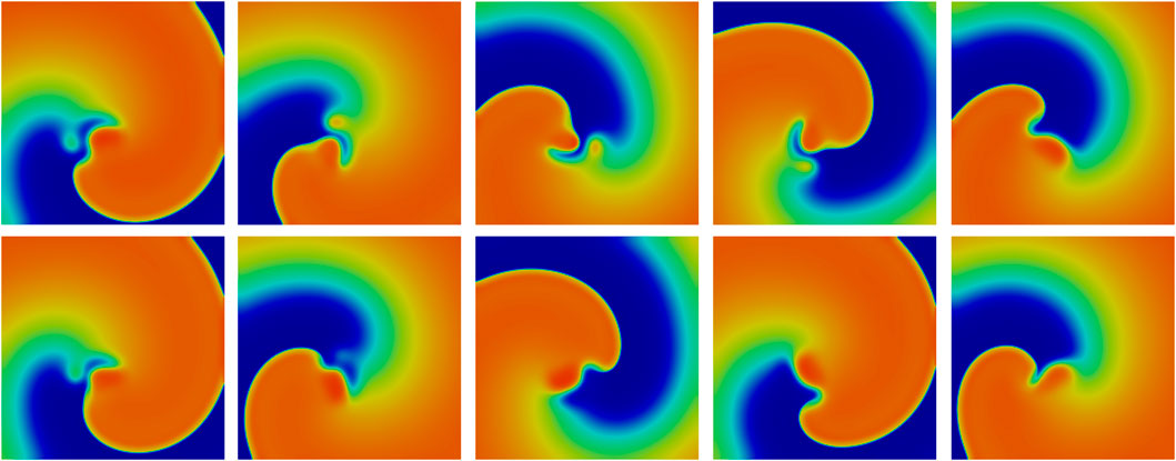
Figure 10. Spiral wave of a normal AP. (First row) normal AP after $2000ms,3000ms,4000ms,5000ms$ and $5400ms$. (Second row) normal AP after $6000ms,7000ms,8000ms,9000ms$ and $10000ms$.

Figure 11

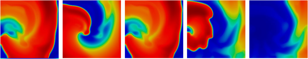
Figure 11. Spiral wave of the EAD, respective wave break-up induced by the EAD at time points $2000ms,3000ms,4000ms,5000ms$ and $5400ms$.

4 Discussion

This paper aims to investigate the complex dynamics of the TP06 model [15, 40], such as the occurrence of action potentials and certain cardiac arrhythmia. While the focus is on early afterdepolarizations (EADs), the approach presented is also applicable to other diseases. A very efficient and beneficial method of studying the behavior of dynamical systems is delivered by bifurcation theory. Thus, one main goal of the paper is the numerical bifurcation analysis of the cellular TP06 model. To this end, we reported the difficulties in modeling the original model, which is also highlighted in [53, 71]. In addition, we discussed several possible modifications and model reductions of the TP06 model which allow numerical bifurcation analysis and apply the numerical continuation algorithm provided in [78, 79]. The aim of model reduction is to simplify a complex mathematical model while retaining its essential behaviors and properties so that the reduced model can be calculated more quickly and analyzed more easily. From an analytical point of view, it is desirable to derive a very simple model; indeed, certain details can be lost, such as on specific ion currents or concentrations, due to the focus on the voltage potential. One specific example is fixing the intracellular potassium concentration ${[K]}_i$. A time-dependent variation of ${[K]}_i$ has only a small effect on the voltage $V$ in this model and causes problems for the bifurcation analysis; however, it might be of importance in certain applications. Thus, we present several steps/levels of model reduction and are able to reduce the 19-dimensional TP06 model to a 14-dimensional version, which has (almost) identical dynamics and trajectories as the original model (cf. Figure 5 and Tables 2–4). This model reduction allows not only performance of numerical bifurcation but also decreases the numerical effort and time. Apart from the steady-state dynamics, which are (almost) identical, it is necessary to adjust the initial stimulus such that the trajectory is able to enter the same basin of attraction. Moreover, Figure 6 illustrates that finding the correct basin of attraction is more difficult for complex dynamics and patterns. On the other hand, we can predict the dynamics of the original TP06 model extract very accurately by analyzing the reduced model. Thus, using the results from a mathematical model which is more feasible and low dimensional for the original model avoids the problem of possible loss of information as long as the approximation reflects the dynamics of the model sufficiently well—which is the case in our study.

After the remodeling, a systematical bifurcation analysis is provided using the set of parameters $({\mathrm{G}}_{\mathrm{K}\mathrm{s}},{\mathrm{G}}_{\mathrm{K}\mathrm{r}},{\mathrm{G}}_{\mathrm{C}\mathrm{a}\mathrm{L}})$, which are known to induce EADs for certain combinations of values (e.g., [7, 8]). This is one aspect for focusing on EADs; another is they are complex voltage oscillations, and therefore this focus provides a better test for the accuracy of our model reduction. Thus, the bifurcation analysis can be seen not only as a tool for analyzing the dynamics of the system but can also be used to test the accuracy of our model reduction. The (numerical) bifurcation analysis shows that the oscillatory behavior of modified TP06 models is induced by an Andronov–Hopf bifurcation, and the occurrence of EADs is related to the existence of an unstable period-doubling bifurcation cascade. In addition, we can conclude oscillatory behavior for the TP06 model from the behavior of the modified models. Moreover, deterministic chaos is not observed, which is in line with [30, 71]. We show that even though the system is in a dangerous region and EADs potentially occur, the initial values and stimulus decide whether the trajectory enters the basin of transient attraction of the period-doubling bifurcation cascade. Therefore, we have three driving forces that induce EADs: the steady-state dynamics of the system related to a combination of a reduced slow and a reduced fast potassium current—${\mathrm{I}}_{{\mathrm{K}}_{\mathrm{s}}}$ and ${\mathrm{I}}_{{\mathrm{K}}_{\mathrm{r}}}$—with an enhanced calcium current ${\mathrm{I}}_{\mathrm{C}\mathrm{a}\mathrm{L}}$, the initial values, and the initial stimulus. This knowledge can now be used to prevent the occurrence of EADs.

Furthermore, to outline the synchronization effects of cardiac cells, we performed numerical experiments highlight how networks of cells 2D-synchronize. Here, we can extract from our investigation how stable patterns appear (Figure 10). In addition, we showed that EADs may induce a wave break-up (Figure 11). While these results show a correlation between EADs and spiral wave breakup, the underlying mechanisms remain complex. A possible explanation is that the prolongation of AP, which often occurs in EADs, increases the heterogeneity of tissue cohesion and refractoriness. This may increase the spatial dispersion of repolarization and thus create the conditions for wavefront fragmentation. In addition, prolonged APs may shorten the effective wavelength of reentrant waves, increasing the chance of wavefront curvature and instability. It is also possible that EADs themselves act as transient depolarization triggers that disrupt the spiral core or interact with the refractory tail of the wavefront to promote breakup. Future research using targeted perturbations and parameter sensitivity analysis will be required to reveal the contributions of these different mechanisms. Moreover, it is highly important to analyze how and when EADs induce wave break-ups resulting in cardiac death. The heart (model) itself contains properties that allow it to stabilize and recover phenomena such as EADs. Here, it is not only the cellular behavior that plays a key role in the geometry of the heart (model) but also its discretization, its diffusivity, and the amount of affect cells that develop EADs.

The main focus of this study has been the model reduction of the cardiac cell model and providing an approach and codes to efficiently investigate cardiac dynamics numerically. These codes can be utilized to investigate different types of arrhythmia and cardiac dynamics on single-cell level. Moreover, it can be used for drug design or to make virtual experiments on the response of cardiac cells or the heart on external influences, such as a pacemaker. We showed on a tissue level that the local steady-state dynamics of the system include certain pattern formations. Furthermore, we discovered that the diffusivity of the system, the initial configuration, and the initial stimulus is highly important for pattern formation and network dynamics. This should be studied in more detail and is part of a future study.

Data availability statement

The raw data supporting the conclusions of this article will be made available by the author without undue reservation.

Author contributions

AE: writing – original draft and writing – review and editing.

Funding

The author(s) declare that financial support was received for the research and/or publication of this article. The author acknowledges the funding by the German Research Foundation (DFG) within the DFG Priority Program SPP 2171 Dynamic Wetting of Flexible, Adaptive, and Switchable Substrates through the project 422786086.

Acknowledgments

The author wishes to thank the referee for the careful reading of the original manuscript and the comments that eventually led to an improved presentation.

Conflict of interest

The author declares that the research was conducted in the absence of any commercial or financial relationships that could be construed as a potential conflict of interest.

Generative AI statement

The author(s) declare that no Generative AI was used in the creation of this manuscript.

Publisher’s note

All claims expressed in this article are solely those of the authors and do not necessarily represent those of their affiliated organizations, or those of the publisher, the editors and the reviewers. Any product that may be evaluated in this article, or claim that may be made by its manufacturer, is not guaranteed or endorsed by the publisher.

Supplementary material

The Supplementary Material for this article can be found online at: https://www.frontiersin.org/articles/10.3389/fphy.2025.1569121/full#supplementary-material

Footnotes

¹Mathematics Subject Classification: 92B25, 92C05, 37G15, 37M05, 37N25

References

1. Tsaneva-Atanasova K, Diaz-Zuccarini V. Editorial: mathematics for healthcare as part of computational medicine. Front Physiol (2018) 9:985. doi:10.3389/fphys.2018.00985

PubMed Abstract | CrossRef Full Text | Google Scholar

2. Xia L, Zhang H, Zheng D. Editorial: multi-scale computational cardiology. Front Physiol (2022) 13:847118. doi:10.3389/.fphys.2022.847118

PubMed Abstract | CrossRef Full Text | Google Scholar

3. Erhardt AH, Tsaneva-Atanasova K, Lines GT, Martens EA. Editorial: dynamical systems, pdes and networks for biomedical applications: mathematical modeling, analysis and simulations. Front Phys (2023) 10. doi:10.338910.3389/fphy.2022.1101756fphy.2022.1101756

PubMed Abstract | CrossRef Full Text | Google Scholar

4. Erhardt AH, Peschka D, Dazzi C, Schmeller L, Petersen A, Checa S, et al. Modeling cellular self-organization in strain-stiffening hydrogels. Comput Mech (2025) 75:875–96. doi:10.1007/s00466-024-02536-7

CrossRef Full Text | Google Scholar

5. Cherry EM, Fenton FH, Krogh-Madsen T, Luther S, Parlitz U. Introduction to focus issue: complex cardiac dynamics. Chaos: Interdiscip J Nonlinear Sci (2017) 27:093701. doi:10.1063/1.5003940

CrossRef Full Text | Google Scholar

6. Erhardt AH, Tsaneva-Atanasova K, Lines GT, Martens EA. In: Dynamical systems, PDEs and networks for biomedical applications: mathematical modeling, analysis and simulations. Lausanne: Frontiers Media SA (2023). doi:10.3389/978-2-83251-458-0

CrossRef Full Text | Google Scholar

7. Van Nieuwenhuyse E, Seemann G, Panfilov AV, Vandersickel N. Effects of early afterdepolarizations on excitation patterns in an accurate model of the human ventricles. PLOS ONE (2017) 12:e0188867–19. doi:10.1371/journal.pone.0188867

PubMed Abstract | CrossRef Full Text | Google Scholar

8. Zimik S, Vandersickel N, Nayak AR, Panfilov AV, Pandit R. A comparative study of early afterdepolarization-mediated fibrillation in two mathematical models for human ventricular cells. PLOS ONE (2015) 10:e0130632–20. doi:10.1371/journal.pone.0130632

PubMed Abstract | CrossRef Full Text | Google Scholar

9. Tveito A, Mardal KA, Rognes ME (2021). Modeling excitable tissue. Springer. doi:10.1007/978-3-030-61157-6

CrossRef Full Text | Google Scholar

10. Mardal KA, Rognes ME, Thompson TB, Valnes LM (2022). Mathematical modeling of the human brain. Springer. doi:10.1007/978-3-030-95136-8

CrossRef Full Text | Google Scholar

11. Niederer SA, Lumens J, Trayanova NA. Computational models in cardiology. Nat Rev Cardiol (2019) 16:100–11. doi:10.1038/s41569-018-0104-y

PubMed Abstract | CrossRef Full Text | Google Scholar

12. Sachse FB Computational cardiology: modeling of anatomy, electrophysiology, and mechanics, 2966. Springer Science and Business Media (2004).

Google Scholar

13. Bueno-Orovio A, Cherry EM, Fenton FH. Minimal model for human ventricular action potentials in tissue. J Theor Biol (2008) 253:544–60. doi:10.1016/j.jtbi.2008.03.029

PubMed Abstract | CrossRef Full Text | Google Scholar

14. Clayton R, Bernus O, Cherry E, Dierckx H, Fenton F, Mirabella L, et al. Models of cardiac tissue electrophysiology: progress, challenges and open questions. Prog Biophys Mol Biol (2011) 104:22–48.

PubMed Abstract | CrossRef Full Text | Google Scholar

15. ten Tusscher KHWJ, Panfilov AV. Alternans and spiral breakup in a human ventricular tissue model. Am J Physiology-Heart Circulatory Physiol (2006) 291:H1088–100. PMID: 16565318. doi:10.1152/ajpheart.00109.2006

PubMed Abstract | CrossRef Full Text | Google Scholar

16. Weiss J, Garfinkel A, Karagueuzian H, Chen P, Qu Z. Early afterdepolarizations and cardiac arrhythmias. Heart Rhythm (2010) 7:1891ff–9. doi:10.1016/j.hrthm.2010.09.017

PubMed Abstract | CrossRef Full Text | Google Scholar

17. Roden D, Viswanathan P. Genetics of acquired long QT syndromeg. J Clin Invest (2005) 115:2025–32. doi:10.1172/.JCI25539

PubMed Abstract | CrossRef Full Text | Google Scholar

18. Fink M, Niederer S, Cherry E, Fenton F, Koivumäki J, Seemann G, et al. Cardiac cell modelling: observations from the heart of the cardiac physiome project. Prog Biophys Mol Biol (2011) 104:2–21. doi:10.1016/j.pbiomolbio.2010.03.002

PubMed Abstract | CrossRef Full Text | Google Scholar

19. Clayton R, Bernus O, Cherry E, Dierckx H, Fenton F, Mirabella L, et al. Models of cardiac tissue electrophysiology: progress, challenges and open questions. Prog Biophys Mol Biol (2011) 104:22–48. doi:10.1016/j.pbiomolbio.2010.05.008

PubMed Abstract | CrossRef Full Text | Google Scholar

20. Kim S, Sato D. Mathematical analysis of the role of heterogeneous distribution of excitable and non-excitable cells on early afterdepolarizations. Front Phys (2018) 6:117. doi:10.3389/fphy.2018.00117

CrossRef Full Text | Google Scholar

21. Barrio R, Martínez MA, Serrano S, Pueyo E. Dynamical mechanism for generation of arrhythmogenic early afterdepolarizations in cardiac myocytes: insights from in silico electrophysiological models. Phys Rev E (2022) 106:024402. doi:10.1103/PhysRevE.106.024402

PubMed Abstract | CrossRef Full Text | Google Scholar

22. Kimrey J, Vo T, Bertram R. Canards underlie both electrical and ca²⁺-induced early afterdepolarizations in a model for cardiac myocytes. SIAM J Appl Dyn Syst (2022) 21:1059–91. doi:10.1137/22M147757X

CrossRef Full Text | Google Scholar

23. Barrio R, Jover-Galtier JA, Martínez M, Pérez L, Serrano S. Mathematical birth of early afterdepolarizations in a cardiomyocyte model. Math Biosciences (2023) 366:109088.

PubMed Abstract | CrossRef Full Text | Google Scholar

24. Tran D, Sato D, Yochelis A, Weiss J, Garfinkel A, Qu Z. Bifurcation and chaos in a model of cardiac early afterdepolarizations. Phys Rev Lett (2009) 102:258103. doi:10.1103/PhysRevLett.102.258103

PubMed Abstract | CrossRef Full Text | Google Scholar

25. Xie Y, Izu L, Bers D, Sato D. Arrhythmogenic transient dynamics in cardiac myocytes. Biophys J (2014) 106:1391–7. doi:10.1016/j.bpj.2013.12.050

PubMed Abstract | CrossRef Full Text | Google Scholar

26. Erhardt AH. Early afterdepolarisations induced by an enhancement in the calcium current. Processes (2019) 7:20. doi:10.3390/pr7010020

CrossRef Full Text | Google Scholar

27. Erhardt AH, Mardal KA, Schreiner JE. Dynamics of a neuron–glia system: the occurrence of seizures and the influence of electroconvulsive stimuli. J Comput Neurosci (2020) 48:229–51. doi:10.1007/s10827-020-00746-5

PubMed Abstract | CrossRef Full Text | Google Scholar

28. Kitajima H, Yazawa T, Barrio R. Fast–slow analysis and bifurcations in the generation of the early afterdepolarization phenomenon in a realistic mathematical human ventricular myocyte model. Chaos: Interdiscip J Nonlinear Sci (2024) 34:123108. doi:10.1063/5.0230834

PubMed Abstract | CrossRef Full Text | Google Scholar

29. Kuehn C. Multiple time scale dynamics. Appl Math Sci (2015) 191. Available online at: https://link.springer.com/book/10.1007/978-3-319-12316-5

Google Scholar

30. Erhardt AH, Solem S. On complex dynamics in a purkinje and a ventricular cardiac cell model. Commun Nonlinear Sci Numer Simulation (2021) 93:105511. doi:10.1016/j.cnsns.2020.105511

CrossRef Full Text | Google Scholar

31. Qu Z. Chaos in the genesis and maintenance of cardiac arrhythmias. Prog Biophys Mol Biol (2011) 105:247–57. doi:10.1016/j.pbiomolbio.2010.11.001

PubMed Abstract | CrossRef Full Text | Google Scholar

32. Dix M, Lilienkamp T, Luther S, Parlitz U. Influence of conduction heterogeneities on transient spatiotemporal chaos in cardiac excitable media. Phys Rev E (2024) 110:044207. doi:10.1103/PhysRevE.110.044207

PubMed Abstract | CrossRef Full Text | Google Scholar

33. Suth D, Luther S, Lilienkamp T. Chaos control in cardiac dynamics: terminating chaotic states with local minima pacing. Front Netw Physiol (2024) 4:1401661. doi:10.3389/fnetp.2024.1401661

PubMed Abstract | CrossRef Full Text | Google Scholar

34. Jæger KH, Charwat V, Charrez B, Finsberg H, Maleckar MM, Wall S, et al. Improved computational identification of drug response using optical measurements of human stem cell derived cardiomyocytes in microphysiological systems. Front Pharmacol (2020) 10:1648. doi:10.3389/fphar.2019.01648

PubMed Abstract | CrossRef Full Text | Google Scholar

35. Tveito A, Maleckar MM, Lines GT. Computing optimal properties of drugs using mathematical models of single channel dynamics. Comput Math Biophys 6 (2018) 41–64. doi:10.1515/cmb-2018-0004

CrossRef Full Text | Google Scholar

36. Zhou X, Qu Y, Passini E, Bueno-Orovio A, Liu Y, Vargas HM, et al. Blinded in silico drug trial reveals the minimum set of ion channels for torsades de pointes risk assessment. Front Pharmacol (2020) 10:1643. doi:10.3389/fphar.2019.01643

PubMed Abstract | CrossRef Full Text | Google Scholar

37. Margara F, Wang ZJ, Levrero-Florencio F, Santiago A, Vázquez M, Bueno-Orovio A, et al. In-silico human electro-mechanical ventricular modelling and simulation for drug-induced pro-arrhythmia and inotropic risk assessment. Prog Biophys Mol Biol (2021) 159:58–74. doi:10.1016/j.pbiomolbio.2020.06.007

PubMed Abstract | CrossRef Full Text | Google Scholar

38. Passini E, Zhou X, Trovato C, Britton OJ, Bueno-Orovio A, Rodriguez B. The virtual assay software for human in silico drug trials to augment drug cardiac testing. J Comput Sci (2021) 52:101202. doi:10.1016/j.jocs.2020.101202

CrossRef Full Text | Google Scholar

39. Pravdin SF, Epanchintsev TI, Panfilov AV. Overdrive pacing of spiral waves in a model of human ventricular tissue. Scientific Rep (2020) 10:20632. doi:10.1038/s41598-020-77314-5

PubMed Abstract | CrossRef Full Text | Google Scholar

40. ten Tusscher KHWJ, Noble D, Noble PJ, Panfilov AV. A model for human ventricular tissue. Am J Physiology-Heart Circulatory Physiol (2004) 286:H1573–89. PMID: 14656705. doi:10.1152/ajpheart.00794.2003

PubMed Abstract | CrossRef Full Text | Google Scholar

41. Hodgkin AL, Huxley AF. A quantitative description of membrane current and its application to conduction and excitation in nerve. J Physiol (1952) 117:500–44. doi:10.1113/jphysiol.1952.sp004764

PubMed Abstract | CrossRef Full Text | Google Scholar

42. Erhardt AH. Cardiac dynamics of a human ventricular tissue model with focus on early afterdepolarizations (2024). Available online at: https://github.com/andreerhardt/cardiac-dynamics-of-a-human-ventricular-tissue-model-with-focus-on-early-afterdepolarizations.

Google Scholar

43. Sundnes J, Lines G, Nielsen B, Mardal KA, Tveito A (2006). Computing the electrical activity in the heart. Springer. doi:10.1007/3-540-33437-8

CrossRef Full Text | Google Scholar

44. Ellingsrud AJ, Solbrå A, Einevoll GT, Halnes G, Rognes ME. Finite element simulation of ionic electrodiffusion in cellular geometries. Front Neuroinformatics (2020) 14:11. doi:10.3389/fninf.2020.00011

PubMed Abstract | CrossRef Full Text | Google Scholar

45. Benedusi P, Ellingsrud AJ, Herlyng H, Rognes ME. Scalable approximation and solvers for ionic electrodiffusion in cellular geometries. SIAM J Scientific Comput (2024) 46:B725–51. doi:10.1137/24M1644717

CrossRef Full Text | Google Scholar

46. Tveito A, Jæger KH, Kuchta M, Mardal KA, Rognes ME. A cell-based framework for numerical modeling of electrical conduction in cardiac tissue. Front Phys (2017) 5. doi:10.3389/fphy.2017.00048

CrossRef Full Text | Google Scholar

47. Jæger KH, Hustad KG, Cai X, Tveito A. Efficient numerical solution of the emi model representing the extracellular space (e), cell membrane (m) and intracellular space (i) of a collection of cardiac cells. Front Phys (2021) 8. doi:10.3389/fphy.2020.579461

CrossRef Full Text | Google Scholar

48. Jæger KH, Tveito A. Deriving the bidomain model of cardiac electrophysiology from a cell-based model; properties and comparisons. Front Physiol (2022) 12:811029. doi:10.3389/fphys.2021.811029

PubMed Abstract | CrossRef Full Text | Google Scholar

49. Mulimani MK, Zimik S, Pandit R. An in silico study of electrophysiological parameters that affect the spiral-wave frequency in mathematical models for cardiac tissue. Front Phys (2022) 9. doi:10.3389/fphy.2021.819873

CrossRef Full Text | Google Scholar

50. Lawson BA, dos Santos RW, Turner IW, Bueno-Orovio A, Burrage P, Burrage K. Homogenisation for the monodomain model in the presence of microscopic fibrotic structures. Commun Nonlinear Sci Numer Simulation (2023) 116:106794. doi:10.1016/j.cnsns.2022.106794

PubMed Abstract | CrossRef Full Text | Google Scholar

51. Alonso S, Bär M, Echebarria B. Nonlinear physics of electrical wave propagation in the heart: a review. Rep Prog Phys (2016) 79:096601. doi:10.1088/0034-4885/79/9/096601

PubMed Abstract | CrossRef Full Text | Google Scholar

52. Luo CH, Rudy Y. A model of the ventricular cardiac action potential. depolarization, repolarization, and their interaction. Circ Res (1991) 68:1501–26. doi:10.1161/01.RES.68.6.1501

PubMed Abstract | CrossRef Full Text | Google Scholar

53. Rose P, Schleimer JH, Schreiber S. Modifications of sodium channel voltage dependence induce arrhythmia-favouring dynamics of cardiac action potentials. PLOS ONE (2020) 15:e0236949–14. doi:10.1371/journal.pone.0236949

PubMed Abstract | CrossRef Full Text | Google Scholar

54. Kuznetsov YA. Elements of applied bifurcation theory. New York: Springer-Verlag (2004). doi:10.1007/.978-1-4757-3978-7

CrossRef Full Text | Google Scholar

55. Fenichel N. Geometric singular perturbation theory for ordinary differential equations. J Differ Equ (1979) 31:53–98. doi:10.1016/0022-0396(79)90152-9

CrossRef Full Text | Google Scholar

56. Tsumoto K, Shimamoto T, Aoji Y, Himeno Y, Kuda Y, Tanida M, et al. Theoretical prediction of early afterdepolarization-evoked triggered activity formation initiating ventricular reentrant arrhythmias. Computer Methods Programs Biomed (2023) 240:107722. doi:10.1016/j.cmpb.2023.107722

PubMed Abstract | CrossRef Full Text | Google Scholar

57. Barrio R, Jover-Galtier J, Martínez M, Pérez L, Serrano S. Mathematical birth of early afterdepolarizations in a cardiomyocyte model. Math Biosciences (2023) 366:109088. doi:10.1016/j.mbs.2023.109088

PubMed Abstract | CrossRef Full Text | Google Scholar

58. Tsumoto K, Kurata Y. Bifurcations and proarrhythmic behaviors in cardiac electrical excitations. Biomolecules (2022) 12:459. doi:10.3390/biom12030459

PubMed Abstract | CrossRef Full Text | Google Scholar

59. Kurata Y, Tsumoto K, Hayashi K, Hisatome I, Kuda Y, Tanida M. Multiple dynamical mechanisms of phase-2 early afterdepolarizations in a human ventricular myocyte model: involvement of spontaneous sr ca2+release. Front Physiol (2020) 10:1545. doi:10.3389/fphys.2019.01545

PubMed Abstract | CrossRef Full Text | Google Scholar

60. Kitajima H, Yazawa T. Bifurcation analysis on a generation of early afterdepolarization in a mathematical cardiac model. Int J Bifurcation Chaos (2021) 31:2150179. doi:10.1142/S0218127421501790

CrossRef Full Text | Google Scholar

61. Tsumoto K, Kurata Y, Furutani K, Kurachi Y. Hysteretic dynamics of multi-stable early afterdepolarisations with repolarisation reserve attenuation: a potential dynamical mechanism for cardiac arrhythmias. Scientific Rep (2017) 7:10771. doi:10.1038/s41598-017-11355-1

PubMed Abstract | CrossRef Full Text | Google Scholar

62. Kimrey J, Vo T, Bertram R. Big ducks in the heart: canard analysis can explain large early afterdepolarizations in cardiomyocytes. SIAM J Appl Dynamical Syst (2020) 19:1701–35. doi:10.1137/19M1300777

CrossRef Full Text | Google Scholar

63. Barrio R, Martínez MA, Pueyo E, Serrano S. Dynamical analysis of early afterdepolarization patterns in a biophysically detailed cardiac model. Chaos: Interdiscip J Nonlinear Sci (2021) 31:073137. doi:10.1063/5.0055965

PubMed Abstract | CrossRef Full Text | Google Scholar

64. Diekman CO, Wei N. Circadian rhythms of early afterdepolarizations and ventricular arrhythmias in a cardiomyocyte model. Biophysical J (2021) 120:319–33. doi:10.1016/j.bpj.2020.11.2264

PubMed Abstract | CrossRef Full Text | Google Scholar

65. Otte S, Berg S, Luther S, Parlitz U. Bifurcations, chaos, and sensitivity to parameter variations in the sato cardiac cell model. Commun Nonlinear Sci Numer Simulation (2016) 37:265–81. doi:10.1016/.j.cnsns.2016.01.014

CrossRef Full Text | Google Scholar

66. Peirlinck M, Costabal F, Yao J, Guccione JM, Tripathy S, Wang Y, et al. Precision medicine in human heart modeling. Biomech Model Mechanobiol (2021) 20:803–31. doi:10.1007/s10237-021-01421-z

PubMed Abstract | CrossRef Full Text | Google Scholar

67. Trayanova NA, Boyle PM. Advances in modeling ventricular arrhythmias: from mechanisms to the clinic. WIREs Syst Biol Med (2014) 6:209–24. doi:10.1002/wsbm.1256

PubMed Abstract | CrossRef Full Text | Google Scholar

68. Trayanova NA, Doshi AN, Prakosa A. How personalized heart modeling can help treatment of lethal arrhythmias: a focus on ventricular tachycardia ablation strategies in post-infarction patients. WIREs Syst Biol Med (2020) 12:e1477. doi:10.1002/wsbm.1477

PubMed Abstract | CrossRef Full Text | Google Scholar

69. Dasí A, Roy A, Sachetto R, Camps J, Bueno-Orovio A, Rodriguez B. In-silico drug trials for precision medicine in atrial fibrillation: from ionic mechanisms to electrocardiogram-based predictions in structurally-healthy human atria. Front Physiol (2022) 13:966046. doi:10.3389/fphys.2022.966046

PubMed Abstract | CrossRef Full Text | Google Scholar

70. Trayanova NA, Lyon A, Shade J, Heijman J. Computational modeling of cardiac electrophysiology and arrhythmogenesis: toward clinical translation. Physiol Rev (2023) 104:1265–333. doi:10.1152/physrev.00017.2023

PubMed Abstract | CrossRef Full Text | Google Scholar

71. Erhardt AH, Solem S. Bifurcation analysis of a modified cardiac cell model. SIAM J Appl Dynamical Syst (2022) 21:231–47. doi:10.1137/21M1425359

CrossRef Full Text | Google Scholar

72. Bernus O, Wilders R, Zemlin CW, Verschelde H, Panfilov AV. A computationally efficient electrophysiological model of human ventricular cells. Am J Physiology-Heart Circulatory Physiol (2002) 282:H2296–308. doi:10.1152/ajpheart.00731.2001

PubMed Abstract | CrossRef Full Text | Google Scholar

73. Alnaes MS, Blechta J, Hake J, Johansson A, Kehlet B, Logg A, et al. The FEniCS project version 1.5, 3. Archive of Numerical Software (2015). doi:10.11588/ans.2015.100.20553

CrossRef Full Text | Google Scholar

74. Logg A, Mardal K, Wells GN. Automated solution of differential equations by the finite element method. Springer (2012). doi:10.1007/978-3-642-23099-8

CrossRef Full Text | Google Scholar

75. E Rognes M, E Farrell P, W Funke S, E Hake J, Mc Maleckar M. cbcbeat: an adjoint-enabled framework for computational cardiac electrophysiology. The J Open Source Softw (2017) 2:224. doi:10.21105/joss.00224

CrossRef Full Text | Google Scholar

76. Finsberg H. fenics-beat. zenodo (2024). doi:10.5281/zenodo.13323643

CrossRef Full Text | Google Scholar

77. Rush S, Larsen H. A practical algorithm for solving dynamic membrane equations. IEEE Trans Biomed Eng, 25 (1978) 389–92. doi:10.1109/TBME.1978.326270

PubMed Abstract | CrossRef Full Text | Google Scholar

78. Dhooge A, Govaerts W, Kuznetsov YA. Matcont: a matlab package for numerical bifurcation analysis of odes. ACM Trans Math Softw (2003) 29:141–64. doi:10.1145/779359.779362

CrossRef Full Text | Google Scholar

79. Dhooge A, Govaerts W, Kuznetsov YA, Meijer HGE, Sautois B. New features of the software matcont for bifurcation analysis of dynamical systems. Math Comput Model Dyn Syst (2008) 14:147–75. doi:10.1080/13873950701742754

CrossRef Full Text | Google Scholar

80. Hund TJ, Kucera JP, Otani NF, Rudy Y. Ionic charge conservation and long-term steady state in the Luo–rudy dynamic cell model. Biophysical J (2001) 81:3324–31. doi:10.1016/s0006-3495(01)75965-6

PubMed Abstract | CrossRef Full Text | Google Scholar

81. Tusscher KHWJT, Panfilov AV. Cell model for efficient simulation of wave propagation in human ventricular tissue under normal and pathological conditions. Phys Med and Biol (2006) 51:6141–56. doi:10.1088/0031-9155/51/23/014

CrossRef Full Text | Google Scholar

82. Erhardt AH. Bifurcation analysis of a certain Hodgkin–Huxley model depending on multiple bifurcation parameters. Mathematics (2018) 6:103–15. doi:10.3390/math6060103

CrossRef Full Text | Google Scholar