Impact of small- and meso-scale electromagnetic field variability on the high-latitude energy input

In this study, the high-resolution data from the Defense Meteorological Satellite Program (DMSP) satellites are used to investigate the contribution and impact of small- and meso-scale electromagnetic field variability with different scales on the estimation of Joule heating and Poynting flux. Smoothing windows with various sizes, such as 5°, 2.5°, 1° magnetic latitude, are used to analyze the characteristics of electromagnetic field variability during the March 2015 geomagnetic storm event. The results show that the small- and meso-scale filed variability can either increase or decrease the estimation of the total Joule heating and Poynting flux during the storm main phase by more than 100% with a smoothing window size of 5° latitude. During the whole period of this storm event, the electric field variability with scales smaller than 5° latitude accounts for 47% of the total electric field on average, whereas the magnetic field variability with scales smaller than 5° latitude only takes 10% of the total magnetic field. Moreover, the mean magnitude changes of Joule heating and Poynting flux due to small- and meso-scale electromagnetic field variability are 58% and 52%, respectively. The impact of small- and meso-scale field variabilities on the energy estimation decreases when smaller smoothing windows are applied, for example, with a size of 0.1° latitude window, the mean magnitude changes of Joule heating and Poynting flux are 20% and 17%, respectively. This demonstrates that finer grids can capture more contribution of small- and meso-scale variabilities in the calculation of Joule heating and Poynting flux. It is very important to use high-resolution grids to calculate the total energy input at high latitudes during storm events. These results will help improve the estimation of high-latitude energy input in the general circulation models, thereby more accurately predict the changes in upper atmospheric parameters.

1 Introduction

The deposition and dissipation processes of solar wind energy in the high-latitude upper atmosphere have been increasingly studied with the growing attention to space weather. During geomagnetic storms, the energy input to the Earth’s upper atmosphere mainly occurs at high latitudes due to the interaction between the solar wind and the Magnetosphere-Ionosphere-Thermosphere (MIT) system. When the solar wind energy is injected into the coupled MIT system, its effect on the thermosphere and ionosphere is related not only to the total amount of energy input, but also to the distribution of energy [1, 2]. Energy flow is an important aspect of magnetosphere-ionosphere coupling. Poynting flux (PF) and particle precipitation are the important forms of high-latitude energy deposition. Poynting flux is the main form of energy dissipation into the upper atmosphere by the solar wind, while the process of particle precipitation not only injects a large amount of energy in the form of heat, but also ionizes the neutral atmosphere and changes the conductivity distribution, thus controlling the spatial distribution of energy dissipation [2–4]. Most of this energy is dissipated in the form of Joule Heating (JH), which has a global impact on the upper atmosphere, such as the enhancement of global neutral atmospheric density, temperature, and atmospheric circulation from the high-latitude regions to the equator [5–11].

Accurate estimation of the high-latitude Poynting flux and Joule heating requires precise measurements of the electric and magnetic fields. The temporal variation and spatial distribution of electric and magnetic fields in the high-latitude ionosphere have been studied for decades. On the large scale of thousands of kilometers, the Dungey circulation convection in the magnetosphere drives Field-Aligned Currents (FACs) and ionospheric plasma convection [12–16]. The typical characteristics of the quasi-static or large-scale processes are controlled by the direction of the Interplanetary Magnetic Field (IMF) [17, 18]. Most commonly used high-latitude electric potential models, such as Weimer05 model [19] and Heelis model [20], assume that the electric field is relatively smooth in space and time, and only take the large-scale electric fields into account for the calculations of Poynting flux and Joule heating. However, the electric field has strong spatial and temporal variability with small- and meso-scales (tens of kilometers and hundreds of kilometers, respectively), which are difficult to estimate and are usually ignored [16, 21].

Codrescu et al. [22] demonstrated for the first time that the difference between the ion drift velocity measurements continuously obtained by the Millstone Hill incoherent scatter radar, and further proposed that the electric field variability can significantly increase Joule heating. Since then, many papers have studied the electric field variability. Matsuo et al. [23] analyzed the measurements of the DE-2 satellite and found that the electric field variability can be comparable to or even greater than the average electric field. As a result, the electric field variability component can contribute as much Joule heating as the average electric field. Johnson and Heelis [24] found that due to the electric field variability in space, the enhancement of Joule heating by spatial structures below 1.28° Magnetic Latitude (MLat) can reach 10%.

Codrescu et al. [25] recalculated the large-scale average electric field and small-scale electric field variability, and substituted them into the Coupled Thermosphere Ionosphere Model (CTIM) to calculate Joule heating. With the additional electric field variability taken into account, Joule heating was significantly enhanced by nearly 100%. Codrescu and Matsuo [26] used the above electric field variability as additional inputs to the Coupled Thermosphere-Ionosphere-Plasmasphere Electrodynamics (CTIPe, [27]) model to study the effects of polar-area electric field variability on the thermosphere and ionosphere during geomagnetically quiet periods. It was found that the impact of small-scale electric field variability to the CTIPe model led to non-negligible Joule heating at high latitudes. Deng and Ridley [28] also analyzed the reasons why existing models underestimate Joule heating and found that both electric field variability and spatial resolution can affect the estimation of Joule heating. Zhu et al. [29] developed a new high-altitude empirical model called Auroral energy Spectrum and High-Latitude Electric field variabilit Y (ASHLEY), which provides a new method for studying the contribution of small-scale electric field variability to high-altitude energy inputs. The additional energy input produced by the presence of the small- and meso-scale variabilities have also been studied by Sheng et al. [30], using the data from the Super Dual Auroral Radar Network (SuperDARN) to drive a global ionosphere-thermosphere model (GITM), and it was found that multi-scale convection forcing increases the regional Joule heating by ∼30% on average, which is mostly contributed by the meso-scale component. In TIEGCM, one of most commonly used General Circulation Models (GCMs), the default spatial resolution is 5° $\times$ 5° (latitude $\times$ longitude), and in the estimation of total heating energy, the Joule heating term is multiplied by a factor of 1.5 to take into account the heating due to small-scale electric field (https://www.hao.ucar.edu/modeling/tgcm/doc/description/model_description.pdf).

In the earliest research paper on electric field variability [22], the ion drift velocity data of the Millstone Hill incoherent scattering radar were studied. The ion drift velocity was used to represent the electric field, and the difference between consecutive ion-drift measurements at the same location versus ion drift was used to demonstrate the electric field variability. Matsuo et al. [31] defined electric field variability as the difference between the true value and the climatological electric field, which is determined through statistical or mathematical methods.

Recently, Weimer [32] suggested the possibility that these variations in the electric field may not be as significant as generally thought. In their study, the problem of fixed conductivity in the calculation of Joule heating in previous studies was discussed, ignoring the anti-correlation between electric field and conductivity. Weimer also pointed out that the simultaneous measurements of electric and magnetic fields when calculating Poynting flux will help to diminish the problem of not knowing conductance values.

The impact of electric and magnetic field variability at different scales (5°, 2.5°, 1° MLat, etc.) including meso- and small-scale on the estimation of Poynting flux and Joule heating is studied using the simultaneous measurements of electric and magnetic fields from Defense Meteorological Satellite Program (DMSP) satellites. The results will help improve the estimation of high-latitude energy input in the existing atmospheric GCMs, thereby improve the prediction of upper atmospheric parameters.

2 Data and methodology

2.1 DMSP data

DMSP satellite data are obtained from the Madrigal website (www.cedar.openmadrigal.org). The data from the Special Sensor for Ions Electrons and Scintillations (SSIES) and Special Sensor for Magnetic Fields (SSM) instruments of DMSP satellites are used in this study, with a temporal resolution of 1 s. SSIES consists of a spherical Langmuir probe mounted on a 0.25-m boom to measure the temperature and density of ambient electrons, and three sensors mounted in different directions on the same conductive plate plane. The three sensors are (1) Ion Trap to measure the total ion density; (2) Ion Drift Meter (IDM) to measure the horizontal ($V_H$) and vertical ($V_V$) drift components of the plasma and the vertical orbit, and (3) Retarding Potential Analyzer (RPA) to measure the ion temperature and the plasma drift component along the orbit ($V_K$). Due to the high sensitivity of the velocity measurement along the orbit and the uncertainty of the potential of the planar conductive plate, the $V_K$ measured by the RPA usually has errors and is therefore not used. In this study, the horizontal ($V_H$) and vertical orbit plasma drift component data with a time resolution of 1 s are used. SSM samples 12 times per second. The data is stored as ${∆B}_X$, ${∆B}_Y$ and ${∆B}_Z$, where $∆B=B_{means}-B_{IGRF}$, which represents the difference between the 1-s average value ($B_{means}$) of the magnetic field measurement at the spacecraft’s location and the local International Geomagnetic Reference Field (IGRF-13) value ($B_{IGRF}$). The orthogonal coordinate system takes the spacecraft’s center of mass as the origin, the X-axis points to the lowest point of the spacecraft, the Y-axis points to the velocity direction, and the Z-axis satisfies the right-hand rule.

The IMF, solar wind and geomagnetic activity index data with a temporal resolution of 1 min are obtained from the OMNI (https://omniweb.gsfc.nasa.gov/) website.

2.2 Calibration of the ion drift velocity

During analysis, we found that the horizontal drift speed of ions in low- and mid-latitude regions (magnetic latitude around 45°) reaches hundreds of meters per second. Theoretically, the horizontal drift speed of ions in low- and mid-latitude regions should be close to zero. We found that this is because the data used was not calibrated, led to inaccurate identification of the Convection Reversal Boundary (CRB). Therefore, we calibrate the data to remove the offset in the original data.

We refer to the method of removing offset from DMSP satellite data used by Hairston and Heelis [33, 34], Rich and Hairston [35], and the method of removing data offset from Swarm satellite data used by [36] and Lomidze et al. [37] to complete the calibration of DMSP satellite ion horizontal drift velocity data. The specific calibration method is as follows.

a)For each trajectory, the magnetic latitude of 45° is taken as the start and end point of the trajectory. The median of the ion horizontal drift velocity 30 s before and after the start and end points is taken as the velocity deviation $∆v_1$ and $∆v_2$. As shown in Equation 1:

$∆v=median\left\{v\right\}(1)$

b) If the velocity offset is too large, that is, $∆v>0.25\times \left[\mathit{max}\left(v\right)-\mathit{min}\left(v\right)\right]$ , the data quality of this trajectory is considered to be poor and this trajectory is discarded.

c) Distribute the velocity offset linearly over the entire trajectory so that the ion horizontal drift velocity at the start and end points is zero. The specific process is shown in Equations 2, 3.

$\delta v=\frac{∆v_1\left(L_0-L_1\right)}{L_0}+∆v_2\left(1-\frac{L_0-L_1}{L_0}\right)(2)$

$v_{new}=v-\delta v(3)$

Where $\delta v$ represents the velocity offset of the linear distribution, $L_0$ represents the distance from the start point to the end point of the trajectory, $L_1$ represents the distance from the start point of the trajectory to the present, and $v_{new}$ represents the horizontal drift velocity of the ion after removing the velocity offset.

Figure 1 is an example of ion horizontal drift velocity data calibration. The figure shows the ion drift velocity of the DMSP F16 satellite from 07:44 to 08:08 UT on 17 March 2015. The black line is the data before calibration, and the blue line is the data after calibration. We can see that there is an obvious offset in the left boundary between the velocity before and after calibration, which may cause errors in subsequent electric field calculations unless removed.

Figure 1

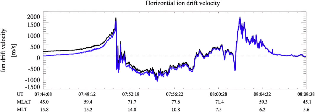
Figure 1. Ion drift velocity from the DMSP F16 satellite during 07:44–08:08 UT on 17 March 2015.

2.3 Calculation of the small- and meso-scale electromagnetic field variability

In this paper, using the definitions of small- and meso-scales from Sheng et al. [30] and Weimer [32], the range of 100–500 km is defined as meso-scale, and the range less than 100 km is defined as small-scale. And the electromagnetic variability determined in this paper is based on a similar definition like Codrescu et al. in 1995.

The electric field is calculated using the calibrated ion drift velocity data and the magnetic field data measured by the SSM instrument according to the electric field calculation formula $\mathit{E}=-\mathit{V}\times \mathit{B}$. Then a smoothing window size is set to smooth the electric field and obtain the average large-scale electric field $E_L$. Next, the actual electric field E is subtracted from the average electric field $E_L$ to obtain the small- and meso-scale electric field variability $E_S=E-E_L$.

Figure 2 shows the electric field observed by the DMSP F16 satellite during 07:45 UT and 08:07 UT on 17 March 2015. Figure (a) is the total electric field E calculated based on the drift velocity of the F16 satellite ions, Figure (b) is the large-scale average electric field $E_L$ obtained after smoothing with a 5° window, Figure (c) is the corresponding small- and meso-scale electric field variability $E_S$, and Figure (d) is the percentage of small- and meso-scale electric field variability in the total electric field. The two red vertical lines represent the Convection Reversal Boundaries (CRBs), which is the location where the plasma changes its flow direction. It can be seen from Figure 2 that the electric field has an obvious variability, which can be as large as 100%.

Figure 2

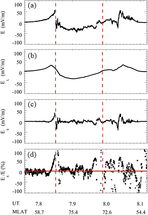
Figure 2. Electric field variations observed by the DMSP F16 satellite from 07:45 UT to 08:07 UT on 17 March 2015. (a) Total electric field E calculated based on the drift velocity of the F16 satellite; (b) Large-scale average electric field E_L obtained using a smoothing window of 5° MLat; (c) The difference between the total electric field and the average electric field, i.e., the small- and meso-scale electric field variability E_S; (d) The percentage of small- and meso-scale electric field variability in the total electric field; The red dashed lines in the figure represent the position of CRBs.

The magnetic field data is processed in the same way. A smoothing window is set and the magnetic field is smoothed at different scales to obtain the average large-scale magnetic field ∆ $B_L$. Then, the difference between the actual magnetic field $∆B$ and the average magnetic field ∆ $B_L$ is used to obtain the small- and meso-scale magnetic field variability ${∆B}_S=∆B-∆B_L$. As shown in Figure 3, the magnetic field variations of the DMSP F16 satellite during 07:45 UT and 08:07 UT on 17 March 2015. Figure (a) is the magnetic field $∆B$ obtained from the F16 satellite observation, Figure (b) is the large-scale average magnetic field $∆B_L$ obtained after smoothing with a 5° window, Figure (c) is the small- and meso-scale magnetic field variability ${∆B}_S$, and Figure (d) is the percentage of small- and meso-scale magnetic field variability in the total magnetic field. In the time period shown in the figure, although the maximum variability of the magnetic field can reach 100%, the fluctuation amplitude is within 20% most of the time.

Figure 3

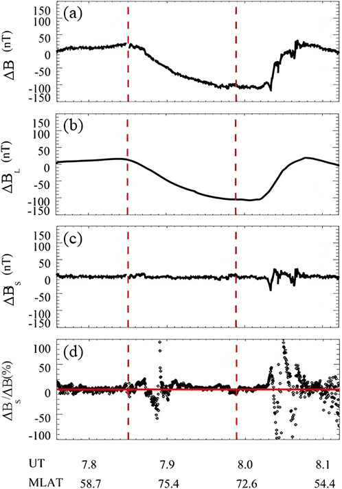
Figure 3. Magnetic field observed by DMSP F16 satellite from 07:45 UT to 08:07 UT on 17 March 2015. (a) Magnetic field ∆B obtained from F16 satellite measurements; (b) Large-scale average magnetic field ∆B_L using a smoothing window of 5° MLat; (c) small- and meso-scale magnetic field variability ∆B_S; (d) Percentage of small- and meso-scale magnetic field variability in the total magnetic field; The red dashed lines in the figure represent the position of CRBs.

Then, the obtained electric field variability is used to calculate the influence of small- and meso-scale electric field variability on Poynting flux and Joule heating. For the high-latitude upper atmosphere energy input, i.e., Poynting flux, it can be rewritten as Equation 4:

$\mathit{S}=\frac{1}{{\mu }_0}\left(\mathit{E}\times ∆\mathit{B}\right)=\frac{1}{{\mu }_0}\left({\mathit{E}}_L\times ∆\mathit{B}+{\mathit{E}}_S\times ∆\mathit{B}\right)(4)$

Then the relative contribution of the small- and meso-scale electric field variability to the Poynting flux is $\left({\mathit{E}}_{\mathit{S}}\times ∆\mathit{B}\right)/\left(\mathit{E}\times ∆\mathit{B}\right).$

If the case where the magnetic field also has small- and meso-scale variability is considered, then the Equation 4 can be rewritten as Equation 5:

$\mathit{S}=\frac{1}{{\mu }_0}\left(\mathit{E}\times ∆\mathit{B}\right)=\frac{1}{{\mu }_0}\left({\mathit{E}}_L\times ∆\mathit{B}+{\mathit{E}}_S\times ∆\mathit{B}\right)=\frac{1}{{\mu }_0}\left({\mathit{E}}_L\times {∆\mathit{B}}_L+{\mathit{E}}_L\times {∆\mathit{B}}_S+{\mathit{E}}_S\times {∆\mathit{B}}_L+{\mathit{E}}_S\times {∆\mathit{B}}_S\right)(5)$

Then the relative contribution of the electromagnetic field variability to the Poynting flux is $\left({\mathit{E}}_{\mathit{L}}\times {∆\mathit{B}}_{\mathit{S}}+{\mathit{E}}_{\mathit{S}}\times {∆\mathit{B}}_{\mathit{L}}+{\mathit{E}}_{\mathit{S}}\times {∆\mathit{B}}_{\mathit{S}}\right)/$$\left(\mathit{E}\times ∆\mathit{B}\right)$.

Similarly, for high latitude upper atmosphere energy dissipation, i.e., Joule heating can be rewritten as Equation 6:

$Q={\sigma }_P{E}^2={\sigma }_P\left(E_L^2+2E_L{E}_S+E_S^2\right)(6)$

${\sigma }_P$ is the Pedersen conductivity, and the neutral winds are not considered.

Therefore, the relative contribution of the electric field variability to Joule heating can be calculated as $\left(2E_L{E}_S+E_S^2\right)/E^2$.

3 Results

We selected the geomagnetic storm event that occurred from March 16th to 20th, 2015 for a detailed study. During this period, the lowest SYM-H index was around −240 nT. This storm period is divided into three phases: the initial phase from 00:00 UT on March 16th to 04:48 UT on 17th, the main phase from 04:48 UT to 22:47 UT on March 17th and the recovery phase from 22:47 UT on March 17th to 00:00 UT on March 21st). The electric and magnetic field variabilities are analyzed separately. The DMSP satellite data are used to calculate the electric field and set smoothing windows at different scales of 5°,2.5°, 1°, 0.5°, 0.25°, 0.1° MLat to calculate the electric and magnetic field variability at small- and meso-scales and study to compute their impacts on the Poynting flux and the Joule heating estimations.

Figures 4, 5 shows the results for the selected path of the DMSP F16 satellite flying over the high latitudes of the northern hemisphere during the main phase. Figure 4 shows the electric field variations and corresponding results observed by the DMSP F16 satellite from 08:40 UT to 09:02 UT on 17 March 2015. From top to bottom and from left to right, are the total electric field, the average electric field smoothed with 5° magnetic latitude window, the difference between the total electric field and the average electric field, i.e., the small- and meso-scale electric field, the square of the total electric field, the square of the average electric field, the difference between the square of the total electric field and the square of the average electric field, the percentage of the small- and meso-scale electric field in the total electric field, and the percentage of the small- and meso-scale electric field on Joule heating. It can be seen that there are clear deviations from the average electric field with comparable amplitudes, and should not be ignored. It can be further seen that its influence on Joule heating cannot be ignored, and it can increase or decrease Joule heating.

Figure 4

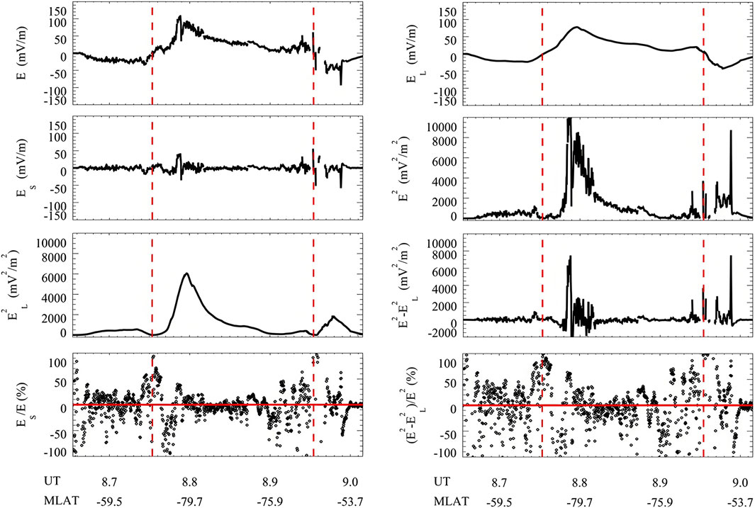
Figure 4. Electric field variations and corresponding results observed by the DMSP F16 satellite from 08:40 UT to 09:02 UT on 17 March 2015. From top to bottom, from left to right, they are the total electric field, the average electric field smoothed with 5° magnetic latitude, the difference between the total electric field and the average electric field, i.e., the small- and meso-scale electric field, the square of the total electric field, the square of the average electric field, the difference between the square of the total electric field and the square of the average electric field, the percentage of the small- and meso-scale electric field in the total electric field, and the percentage of the small- and meso-scale electric field influencing Joule heating.

Figure 5

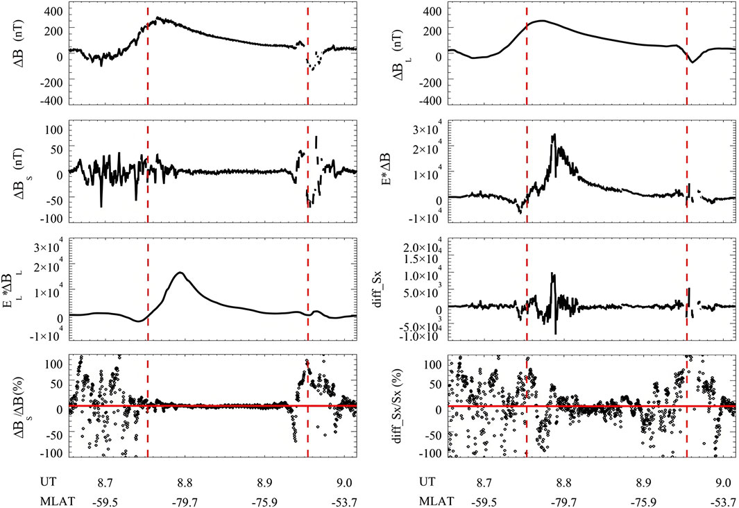
Figure 5. Magnetic field variations and corresponding results observed by the DMSP F16 satellite from 08:40 UT to 09:02 UT on 17 March 2015. From top to bottom, from left to right, they are the total magnetic field ($∆B$), the average magnetic field smoothed with 5° magnetic latitude ($∆B_L$), the difference between the total magnetic field and the average magnetic field, i.e., the small- and meso-scale magnetic field ($∆B_S$), the product of the total electric field and the total magnetic field ($E\times ∆B$), the product of the large-scale electric field and the large-scale magnetic field ($E_L\times ∆B_L$), the product of the total electric field and the total magnetic field minus the product of the large-scale electric field and the large-scale magnetic field ($E\times ∆B-E_L\times ∆B_L$), the percentage of the s small- and meso-scale magnetic field in the total magnetic field ($∆B_S/∆B$), and the percentage of the small- and meso-scale electromagnetic field in the Poynting flux [($E\times ∆B-E_L\times ∆B_L)/\left(E\times ∆B\right)$].

In this study, the Mean Absolute Percentage Error (MAPE) is used to represent the average impact of small- and meso-scale fields to a value in a certain duration, such as the electric field, magnetic field, Joule heating or Poynting flux, as shown in Formula 7.

$MAPE=\frac{1}{n}{\displaystyle \sum _{i=1}^n}\left|\frac{y_i-{\overline{y}}_i}{y_i}\right|\times 100\%(7)$

where n is the number of data considered, $y_i$ is the original value, and ${\overline{y}}_i$ is the averaged or large-scale value. In this particular trajectory during the main phase shown in Figure 4, the MAPE of electric field is 44%, and that of Joule heating is also 44%. This result demonstrates that the average contribution of the small- and meso-scale electric field on Joule heating during this pass is non-negligible.

Figure 5 shows the magnetic field variations and corresponding results observed by the DMSP F16 satellite from 08:40 UT to 09:02 UT on 17 March 2015. From top to bottom, from left to right are the total magnetic field, the average magnetic field smoothed with 5° MLat window, the difference between the total magnetic field and the average magnetic field, i.e., the small- and meso-scale magnetic field, the product of the total electric field and the total magnetic field, the product of the total electric field and the average magnetic field, the difference between the product of the total electric field and the total magnetic field and the product of the total electric field and the average magnetic field, the percentage of the small- and meso-scale magnetic field in the total magnetic field, and the percentage of the small- and meso-scale electromagnetic field on the Poynting flux. There is also variability in the magnetic field, but the magnetic variability is not as large as that of the electric field of the electric field. The magnetic field variations relatively slow for most of the time at high latitudes. On this trajectory, the MAPE of magnetic field is 9%, while that of Poynting flux is 46%. The results indicate that the contribution of the small- and meso-scale variabilities on the Poynting flux is mainly caused by the electric field variability. For this particular path during the storm main phase, if the small- and meso-scale field variabilities were ignored, Poynting flux would be underestimated by almost 50%.

The spatial distribution of the electric field and magnetic field variability observed by the DMSP F16 satellite during the main phase of this magnetic storm, as well as the calculated spatial distribution of Joule heating and Poynting flux are shown in Figures 6, 7 for the high-latitude regions. Compared with the electric field variability, the magnetic field variability is relatively small, and the spatial distribution of the Poynting flux is more consistent with the spatial distribution of the electric field variability. The MAPE of electric field during the main phase is around 35%, whereas the that of magnetic field accounts for 18%. Also, the MAPEs of Joule heating and Joule heating are 46% and 43%, respectively. The variabilities in the northern and southern hemispheres are similar, as shown in Figures 6, 7. Therefore, the results demonstrate that small- and meso-scale electromagnetic field variability should not be ignored in the estimation of high-latitude energy input during storm main phases.

Figure 6

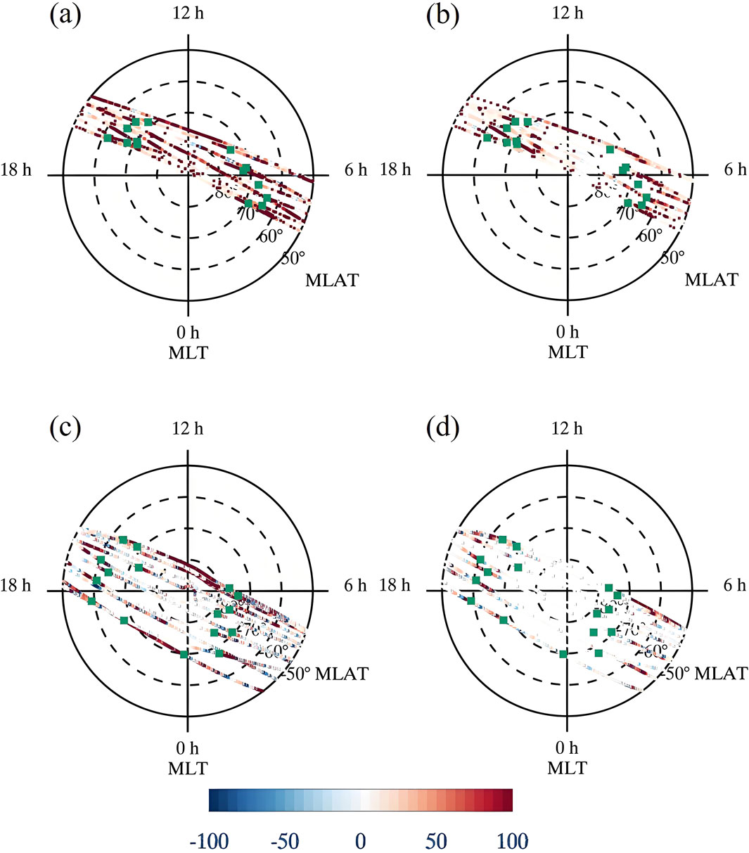
Figure 6. Spatial distribution of small- and meso-scale electromagnetic field variability during the main phase of the magnetic storm on 16 March 2015. The green dots indicate the locations of CRBs. A smoothing window of 5° magnetic latitude is used. (a) E_S/E (%) for northern hemisphere. (b) ∆B_S/∆B (%) for northern hemisphere. (c) E_S/E (%) for southern hemisphere. (d) ∆B_S/∆B (%) for southern hemisphere.

Figure 7

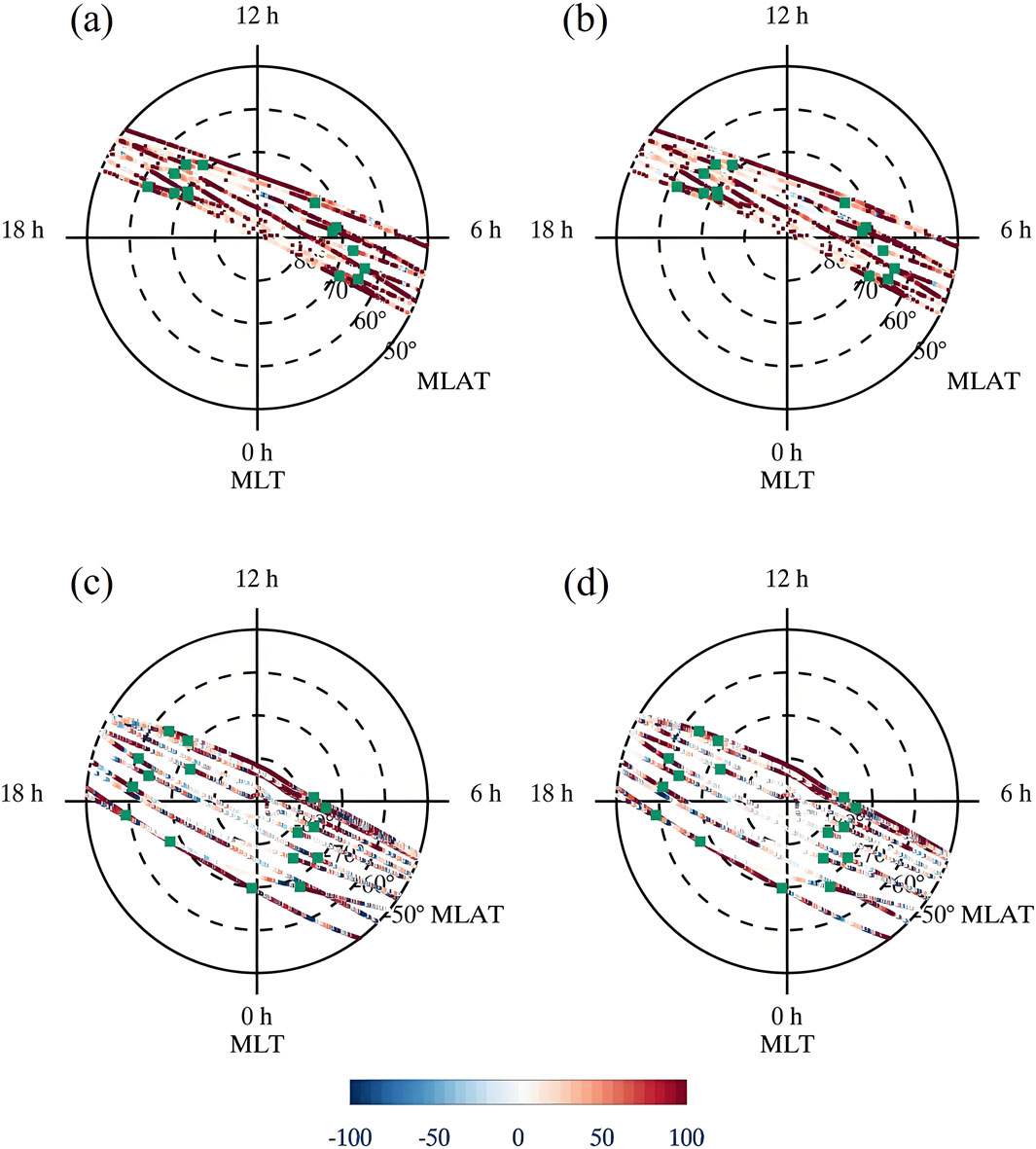
Figure 7. Spatial distribution of the impact of small- and meso-scale electromagnetic field variability on Joule heating and Poynting flux during the magnetic storm on 16 March 2015. The green dots indicate the locations of CRBs. A smoothing window of 5° magnetic latitude is used. (a) (E²-E²L)/E² (%) for northern hemisphere. (b) (E × ∆B-E_L × ∆B_L)/(E × ∆B) (%) for northern hemisphere. (c) (E²-E²_L)/E² (%) for southern hemisphere. (d) (E × ∆B-E_L × ∆B_L)/(E × ∆B) (%) for southern hemisphere.

The green dots in Figures 6, 7 indicate the locations of CRBs, which can be used to illustrate the boundaries between open an closed field lines, in another words, the boundaries between the polar cap and the auroral zone. Only those paths with both CRBs found are considered for the following statical studies. Table 1 demonstrates the statistical results in different regions over the high-latitude regions. It can be seen that during the main phase of this magnetic storm, the contribution of the small-and meso-scale electromagnetic field variability in the auroral zone is larger than that in the polar cap. That is, if only the large-scale electromagnetic field were taken into account in the estimation of high-latitude energy input, Joule heating and Poynting flux would be underestimated by around 30% in the polar cap region, whereas about 50% and 40% underestimation of Joule heating and Poynting flux would occur, respectively, in the auroral zones.

Table 1

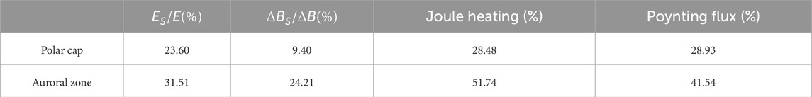
Table 1. Statistical results of the polar cap and auroral zone during the main phase of the magnetic storm on 17 March 2015 (5° MLat smoothing window).

The DMSP F16 data are statistically analyzed according to different magnetic storm phases, and the results are shown in Tables 2–4. Table 2 is the result during the initial phase of the magnetic storm from March 16 to 20, 2015, Table 3 is the result during the main phase of this magnetic storm, and Table 4 is the result during the recovery phase of this storm. It can be seen that when the window is reduced from 5° step by step, the fraction of previously neglected electric field variability decreases. During the main phase, when the window size is reduced from 5° to 0.1°, the MAPE of small- and meso-scale electric field variability is reduced from 35% to 10%, indicating that finer grids can capture more small- and meso-scale variations. When the window is reduced from 5° to 0.5°, the contribution of small- and meso-scale electromagnetic fields to Joule heating and Poynting flux variations are reduced from 46% to 24% and from 43% to 22%, respectively, indicating that more energy is taken into account and the neglected parts have been greatly reduced. Figure 8 is a graphical representation of the data in Tables 2–4, which are the data of the initial phase, main phase and recovery phase of the magnetic storm from top to bottom. From Figure 8, when the smoothing window is smaller, the effect of energy calculation is getting better, and more small- and meso-scale electromagnetic field variabilities are included in the calculation. When we use GCMs to simulate the upper atmosphere, using higher-resolution grids as much as possible can significantly improve the accuracy of the calculated energy input.

Table 2

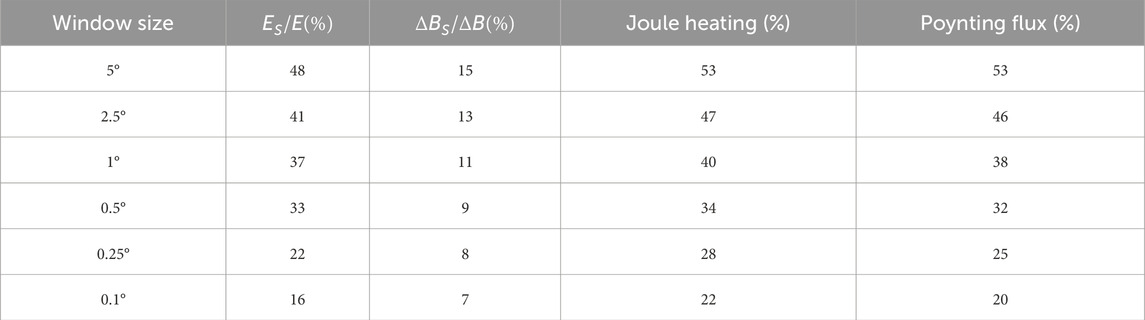
Table 2. DMSP F16 satellite data results of the initial phase of the magnetic storm.

Table 3

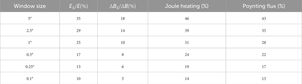
Table 3. DMSP F16 satellite data results of the main phase of the magnetic storm.

Table 4

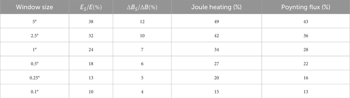
Table 4. DMSP F16 satellite data results of the recovery phase of the magnetic storm.

Figure 8

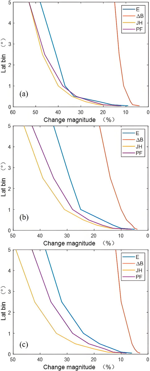
Figure 8. The percentage change of electric field, magnetic field, Joule heating and Poynting flux as a function of window size during the magnetic storm on 16 March 2015. (A) Initial phase of the magnetic storm; (B) Main phase; (C) Recovery phase.

Data from DMSP F16, F17, F18 and F19 satellites are also used to conduct the same analysis for this magnetic storm event. The results are shown in Tables 5–8. The results are similar the same for these satellites, when the smoothing window is smaller, more small- and meso-scale electromagnetic field variabilities are included in the calculation.

Table 5

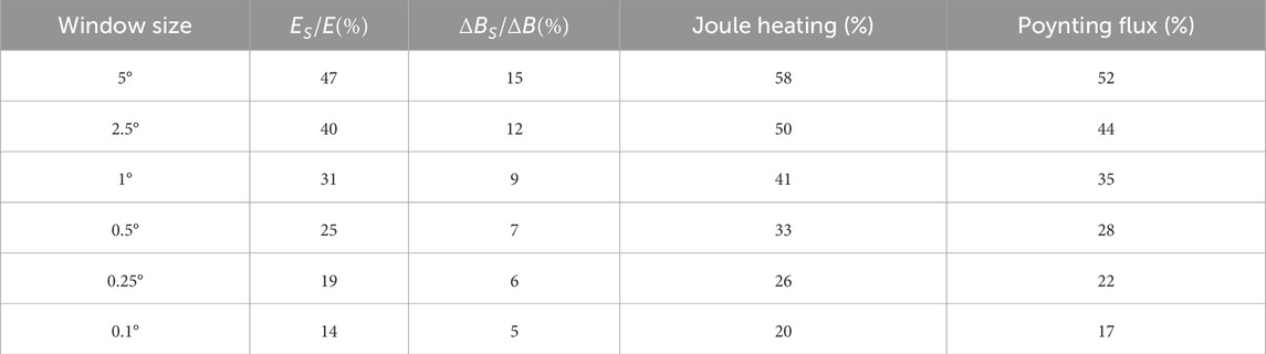
Table 5. DMSP F16 satellite data results during the magnetic storm on 16 March 2015.

Table 6

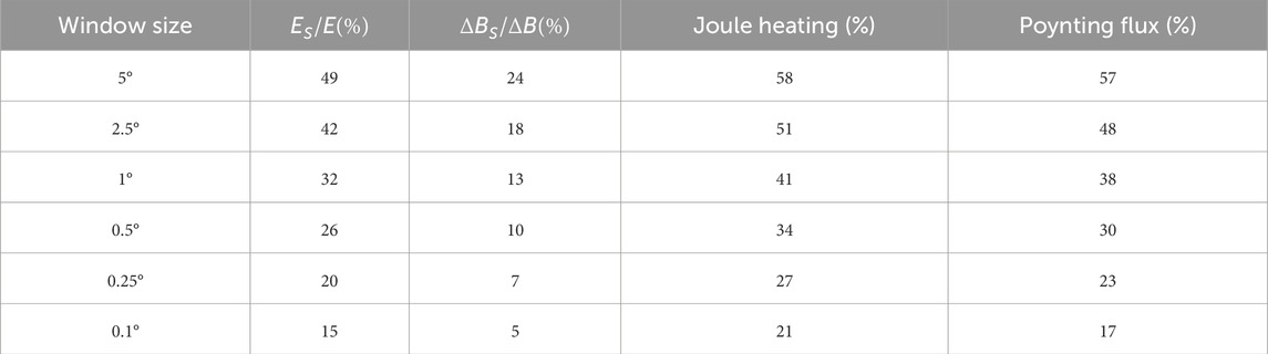
Table 6. DMSP F17 satellite data results during the magnetic storm on 16 March 2015.

Table 7

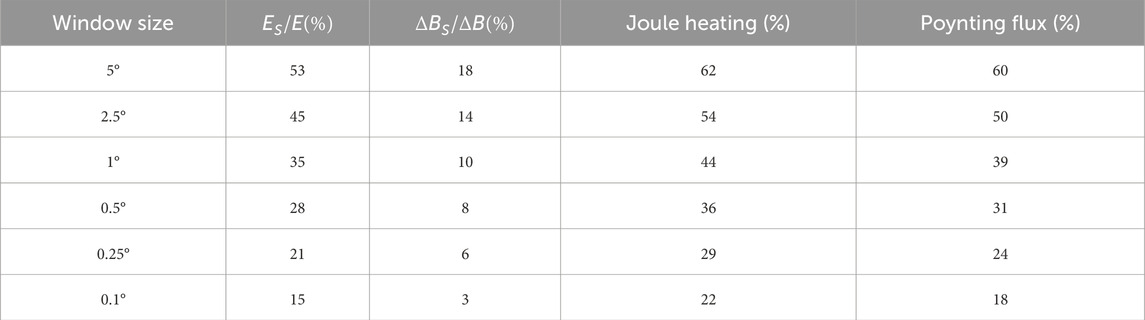
Table 7. DMSP F18 satellite data results during the magnetic storm on 16 March 2015.

Table 8

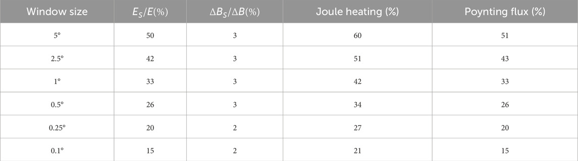
Table 8. DMSP F19 satellite data results during the magnetic storm on 16 March 2015.

4 Discussion and conclusion

In this study, small- and meso-scale electomagnetic field are determined and studied using high-resolution data from the DMSP satellites. The results show that there are non-negligible small and meso-scale electromagnetic field variability, and the magnitude of these variabilities can be comparable to the large-scale average electromagnetic field.

The geomagnetic storm event from March 16 to 20, 2015 is selected to analyze the small- and meso-scale electromagnetic field variability observed from DMSP F16 satellite and their impact on the high-latitude energy input. The fraction of the electric and magnetic field variability that was previously neglected decreased with the decrease of the selected window size, that is, as the window size continues to decrease, more small- and meso-scale electromagnetic field variabilities are considered. Using a smoothing window size of 5° MLat, the small- and meso-scale electric field variability can account for 47% of the total electric field on average, whereas the small- and meso-scale magnetic field variability accounts for about 15% of the total magnetic field. Therefore, the electric field variability plays dominant role affecting the small- and meso-scale variations of Joule heating and Poynting flux. Since finer grids can capture more small- and meso-scale variations, when the smoothing window size gradually decreases from 5° to 0.1°, the MAPE of electric field variability gradually decreases from 47% to 14%, and that of magnetic field decreases from 15% to 5%. The small- and meso-scale variabilities included in the estimation of Joule heating and Poynting flux increase, and the ignored part of Joule heating in the calculation has been reduced from 58% to 20%, and Poynting flux has been reduced from 52% to 17%, respectively. For this particular storm event, when the latitude grid size is 5° MLat and only the large-scale electric and magnetic fields are taken into account, Joule heating is underestimated by 58% and Poynting flux is underestimated by 47%. This might be the reason why there are lack of high-altitude energy input problems in GCMs driven by empirical high-latitude models for storm events, and additional energy is applied intentionally to simulate the correct atmospheric parameters. We also extend the research to other DMSP satellites and find that the conclusions from the four DMSP F16, 17, 18, F19 satellites are consistent.

In addition, we compared the method of using an equal-length window corresponding to 5° MLat with our method of using a 5° MLat fixed-size smoothing window. Both methods yielded similar results. The MAPE of the small- and meso-scale electric field for the pass in Figure 2 was 48% for the fixed-size-window method and 43% for the equal-length window method, indicating no significant impact on Poynting flux estimation.

The results from our study agree with previous studies. With additional electric field variability taken into account, Codrescu et al. [25] found Joule heating was significantly enhanced by nearly 100%. Matsuo et al. [23] found that the electric field variability can be comparable to or even greater than the average electric field. As a result, the electric field variability component may contribute as much Joule heating as the average electric field. Codrescu and Matsuo [26] studied the effects of polar-area electric field variability on the thermosphere and ionosphere during geomagnetically quiet periods, and found that the small-scale electric field variability led to non-negligible Joule heating at high latitudes. The additional energy input produced by the presence of the small- and meso-scale variabilities have also been studied by Sheng et al. [30], and the results demonstrated that multi-scale convection forcing increases the regional Joule heating by ∼30% on average. The default spatial resolution of TIEGCM is 5° $\times$ 5° (latitude $\times$ longitude), and in the estimation of total heating energy, the Joule heating term is multiplied by a factor of 1.5 to take into account the heating due to small-scale electric field. Our research presented in this paper provides further evidence for the critical role of small-and meso-scale variabilities in the estimation of high-latitude energy input.

In this study, we also discuss the question raised by Weimer [32] using the simultaneous observations of electric and magnetic fields to calculate the Poynting flux, in order to avoid the problem of using uncertain conductivity. We find that the meso- and small-scale electric field variability does contribute a lot to the estimation of Joule heating and Poynting flux. Therefore, it is very important to use high-resolution grids to calculate the high-latitude energy input during the geomagnetic storm events, otherwise it is necessary to compensate for the impact of insufficient spatial resolution on energy input. The research results will help improve the energy input of high-latitude regions in the existing atmospheric circulation model, thereby more accurately predicting the changes in upper atmospheric parameters.

Data availability statement

The original contributions presented in the study are included in the article/supplementary material, further inquiries can be directed to the corresponding author.

Author contributions

JJ: Data curation, Formal Analysis, Software, Validation, Visualization, Writing – original draft, Writing – review and editing. YH: Formal Analysis, Methodology, Supervision, Validation, Writing – review and editing.

Funding

The author(s) declare that financial support was received for the research and/or publication of this article. This work is jointly supported by the National Natural Science Foundation of China (Grant 42130210 and 41804152), Shenzhen Science and Technology Program (JCYJ20220818102401003), Shenzhen Key Laboratory Launching Project No. ZDSYS20210702140800001 and Open Research Program of CAS Key Laboratory of Geospace Environment (No. GE2018-01).

Acknowledgments

We acknowledge the Madrigal website (www.cedar.openmadrigal.org) for providing the essential data of DMSP satellites.

Conflict of interest

The authors declare that the research was conducted in the absence of any commercial or financial relationships that could be construed as a potential conflict of interest.

Generative AI statement

The author(s) declare that no Generative AI was used in the creation of this manuscript.

Publisher’s note

All claims expressed in this article are solely those of the authors and do not necessarily represent those of their affiliated organizations, or those of the publisher, the editors and the reviewers. Any product that may be evaluated in this article, or claim that may be made by its manufacturer, is not guaranteed or endorsed by the publisher.

References

1. Lu G, Baker DN, McPherron RL, Farrugia CJ, Lummerzheim D, Ruohoniemi JM, et al. Global energy deposition during the January 1997 magnetic cloud event. J Geophys Research-Space Phys (1998) 103(A6):11685–94. doi:10.1029/98ja00897

CrossRef Full Text | Google Scholar

2. Deng Y, Maute A, Richmond AD, Roble RG. Analysis of thermospheric response to magnetospheric inputs. J Geophys Research-Space Phys (2008) 113(A4). doi:10.1029/2007ja012840

CrossRef Full Text | Google Scholar

3. Prölss GW, Brace LH, Mayr HG, Carignan GR, Killeen TL, Klobuchar JA. Ionospheric storm effects at subauroral latitudes: a case study. J Geophys Res Space Phys (1991) 96(A2):1275–88. doi:10.1029/90JA02326

CrossRef Full Text | Google Scholar

4. Fuller-Rowell TJ, Codrescu MV, Moffett RJ, Quegan S. Response of the thermosphere and ionosphere to geomagnetic storms. J Geophys Res Space Phys (1994) 99(A3):3893–914. doi:10.1029/93JA02015

CrossRef Full Text | Google Scholar

5. Sharber JR, Frahm RA, Link R, Crowley G, Winningham JD, Gaines EE, et al. UARS particle environment monitor observations during the November 1993 storm: auroral morphology, spectral characterization, and energy deposition. J Geophys Research-Space Phys (1998) 103(A11):26307–22. doi:10.1029/98ja01287

CrossRef Full Text | Google Scholar

6. Lühr H, Rother M, Köhler W, Ritter P, Grunwaldt L. Thermospheric up-welling in the cusp region: evidence from CHAMP observations. Geophys Res Lett (2004) 31(6). doi:10.1029/2003GL019314

CrossRef Full Text | Google Scholar

7. Liu H, Lühr H. Strong disturbance of the upper thermospheric density due to magnetic storms: CHAMP observations. J Geophys Res Space Phys (2005) 110(A9). doi:10.1029/2004JA010908

CrossRef Full Text | Google Scholar

8. Vanhamäki H, Yoshikawa A, Amm O, Fujii R. Ionospheric Joule heating and Poynting flux in quasi-static approximation. J Geophys Res Space Phys (2012) 117(A8). doi:10.1029/2012JA017841

CrossRef Full Text | Google Scholar

9. Burns A, Wang W, Solomon S, Qian L. Energetics and composition in the thermosphere. Model Ionosphere–Thermosphere Syst (2014) 39–48. doi:10.1002/9781118704417.ch4

CrossRef Full Text | Google Scholar

10. Fuller-Rowell T. Physical characteristics and modeling of Earth's thermosphere. Model Ionosphere–Thermosphere Syst (2014) 13–27. doi:10.1002/9781118704417.ch2

CrossRef Full Text | Google Scholar

11. Schunk R. Ionosphere-thermosphere physics: current status and problems. Model Ionosphere–Thermosphere Syst (2014) 3–12. doi:10.1002/9781118704417.ch1

CrossRef Full Text | Google Scholar

12. Dungey JW. Interplanetary magnetic field and the auroral zones. Phys Rev Lett (1961) 6(2):47–8. doi:10.1103/physrevlett.6.47

CrossRef Full Text | Google Scholar

13. Iijima T, Potemra TA. Field-aligned currents in the dayside cusp observed by Triad. J Geophys Res (1976) 81(34):5971–9. doi:10.1029/ja081i034p05971

CrossRef Full Text | Google Scholar

14. Cowley SWH, Lockwood M. Excitation and decay of solar wind-driven flows in the magnetosphere-ionospheresystem. Annales Geophysicae (1992) 10(1-2):103–15.

Google Scholar

15. Weimer DR. Maps of ionospheric field-aligned currents as a function of the interplanetary magnetic field derived from Dynamics Explorer 2 data. J Geophys Research-Space Phys (2001) 106(A7):12889–902. doi:10.1029/2000ja000295

CrossRef Full Text | Google Scholar

16. Billett DD, McWilliams KA, Ponomarenko PV, Martin CJ, Knudsen DJ, Vines SK. Multi-scale ionospheric poynting fluxes using ground and space-based observations. Geophys Res Lett (2023) 50(10):e2023GL103733. doi:10.1029/2023GL103733

CrossRef Full Text | Google Scholar

17. Heppner J, Maynard N. Empirical high-latitude electric field models. J Geophys Res Space Phys (1987) 92(A5):4467–89. doi:10.1029/ja092ia05p04467

CrossRef Full Text | Google Scholar

18. Ruohoniemi JM, Greenwald RA. Statistical patterns of high-latitude convection obtained from Goose Bay HF radar observations. J Geophys Research-Space Phys (1996) 101(A10):21743–63. doi:10.1029/96ja01584

CrossRef Full Text | Google Scholar

19. Weimer DR. Improved ionospheric electrodynamic models and application to calculating Joule heating rates. J Geophys Res Space Phys (2005) 110(A5). doi:10.1029/2004JA010884

CrossRef Full Text | Google Scholar

20. Heelis RA, Lowell JK, Spiro RW. A model of the high-latitude ionospheric convection pattern. J Geophys Res Space Phys (1982) 87(A8):6339–45. doi:10.1029/JA087iA08p06339

CrossRef Full Text | Google Scholar

21. Cousins EDP, Matsuo T, Richmond AD. Mesoscale and large-scale variability in high-latitude ionospheric convection: dominant modes and spatial/temporal coherence. J Geophys Research-Space Phys (2013) 118(12):7895–904. doi:10.1002/2013ja019319

CrossRef Full Text | Google Scholar

22. Codrescu MV, Fuller-Rowell TJ, Foster JC. On the importance of E-field variability for Joule heating in the high-latitude thermosphere. Geophys Res Lett (1995) 22(17):2393–6. doi:10.1029/95GL01909

CrossRef Full Text | Google Scholar

23. Matsuo T, Richmond AD, Hensel K. High-latitude ionospheric electric field variability and electric potential derived from DE-2 plasma drift measurements: dependence on IMF and dipole tilt. J Geophys Research-Space Phys (2003) 108(A1). doi:10.1029/2002ja009429

CrossRef Full Text | Google Scholar

24. Johnson ES, Heelis RA. Characteristics of ion velocity structure at high latitudes during steady southward interplanetary magnetic field conditions. J Geophys Research-Space Phys (2005) 110(A12). doi:10.1029/2005ja011130

CrossRef Full Text | Google Scholar

25. Codrescu MV, Fuller-Rowell TJ, Foster JC, Holt JM, Cariglia SJ. Electric field variability associated with the Millstone Hill electric field model. J Geophys Research-Space Phys (2000) 105(A3):5265–73. doi:10.1029/1999ja900463

CrossRef Full Text | Google Scholar

26. Codrescu M, Matsuo T. Auroral E-field variability effects in the ionosphere. In: Ursi (2002).

Google Scholar

27. Fuller-Rowell TJ, Rees D. Derivation of a conservation equation for mean molecular weight for a two-constituent gas within a three-dimensional, time-dependent model of the thermosphere. Planet Space Sci (1983) 31(10):1209–22. doi:10.1016/0032-0633(83)90112-5

CrossRef Full Text | Google Scholar

28. Deng Y, Ridley AJ. Possible reasons for underestimating Joule heating in global models: E field variability, spatial resolution, and vertical velocity. J Geophys Research-Space Phys (2007) 112(A9). doi:10.1029/2006ja012006

CrossRef Full Text | Google Scholar

29. Zhu Q, Deng Y, Maute A, Kilcommons LM, Knipp DJ, Hairston M. ASHLEY: a new empirical model for the high-latitude electron precipitation and electric field. Space Weather-the Int J Res Appl (2021) 19(5). doi:10.1029/2020sw002671

CrossRef Full Text | Google Scholar

30. Sheng C, Deng Y, Bristow WA, Nishimura Y, Heelis RA, Gabrielse C. Multi-scale geomagnetic forcing derived from high-resolution observations and their impacts on the upper atmosphere. Space Weather (2022) 20(12):e2022SW003273. doi:10.1029/2022SW003273

CrossRef Full Text | Google Scholar

31. Matsuo T, Richmond AD, Nychka DW. Modes of high-latitude electric field variability derived from DE-2 measurements: empirical Orthogonal Function (EOF) analysis. Geophys Res Lett (2002) 29(7). doi:10.1029/2001gl014077

CrossRef Full Text | Google Scholar

32. Weimer D. The significance of small-scale electric fields may be overestimated. Front Astron Space Sci (2024) 11. doi:10.3389/fspas.2024.1391990

CrossRef Full Text | Google Scholar

33. Hairston M, Heelis R. Model of the high-latitude ionospheric convection pattern during southward interplanetary magnetic field using DE 2 data. J Geophys Res Space Phys (1990) 95(A3):2333–43. doi:10.1029/ja095ia03p02333

CrossRef Full Text | Google Scholar

34. Hairston MR, Heelis RA. Response time of the polar ionospheric convection pattern to changes in the north-south direction of the IMF. Geophys Res Lett (1995) 22(5):631–4. doi:10.1029/94gl03385

CrossRef Full Text | Google Scholar

35. Rich FJ, Hairston M. LARGE-SCALE CONVECTION PATTERNS OBSERVED BY DMSP. J Geophys Research-Space Phys (1994) 99(A3):3827–44. doi:10.1029/93ja03296

CrossRef Full Text | Google Scholar

36. Fiori RAD, Koustov AV, Boteler DH, Knudsen DJ, Burchill JK. Calibration and assessment of Swarm ion drift measurements using a comparison with a statistical convection model. Earth Planets and Space (2016) 68:100. doi:10.1186/s40623-016-0472-7

CrossRef Full Text | Google Scholar

37. Lomidze L, Burchill JK, Knudsen DJ, Kouznetsov A, Weimer DR. Validity study of the Swarm horizontal cross-track ion drift velocities in the high-latitude ionosphere. Earth Space Sci (2019) 6(3):411–32. doi:10.1029/2018ea000546

CrossRef Full Text | Google Scholar